Sensitivity and Uncertainty Analyses of Human and Organizational Risks in Fire Safety Systems for High-Rise Residential Buildings with Probabilistic T-H-O-Risk Methodology

Abstract

Given that existing fire risk models often ignore human and organizational errors (HOEs) ultimately leading to underestimation of risks by as much as 80%, this study employs a technical-human-organizational risk (T-H-O-Risk) methodology to address knowledge gaps in current state-of-the-art probabilistic risk analysis (PRA) for high-rise residential buildings with the following goals: (1) Develop an improved PRA methodology to address concerns that deterministic, fire engineering approaches significantly underestimate safety levels that lead to inaccurate fire safety levels. (2) Enhance existing fire safety verification methods by incorporating probabilistic risk approach and HOEs for (i) a more inclusive view of risk, and (ii) to overcome the deterministic nature of current verification methods. (3) Perform comprehensive sensitivity and uncertainty analyses to address uncertainties in numerical estimates used in fault tree/event trees, Bayesian network and system dynamics and their propagation in a probabilistic model. (4) Quantification of human and organizational risks for high-rise residential buildings which contributes towards a policy agenda in the direction of a sustainable, risk-based regulatory regime. This research contributes to the development of the next-generation building codes and risk assessment methodologies.

1. Introduction

Probabilistic modelling of fire safety risks in high-rise residential buildings typically has included technical risks and errors, while ignoring the impacts of human and organizational risks resulting in significant underestimation of overall risks. It has been well recognized that human and organizational factors (HOFs) are the leading causes of most accidents, and literature in other related industries indicates that existing models that ignore human and organizational errors (HOEs) underestimate risk, possibly by as much as 80% [1,2,3]. From a practical viewpoint, it is essential to adopt technical, human, and organizational risks for a realistic fire risk assessment of a building design [2]. Moreover, during the operational phase of a building, the reliability of the fire equipment should not be considered constant, and its aging over time must be addressed to derive more realistic risk values [4]. Prior studies provide estimated effects of HOEs on risk in other industries such as nuclear plants, aviation and offshore oil platforms, but existing literature does not address or quantify the impact of HOEs on risks during fire events in high-rise buildings.

Recent fatalities in high-rise residential fires, e.g., Grenfell, London, have demonstrated the urgent need to consider HOEs in probabilistic risk assessments (PRA) for high-rise residential buildings [2,5]. However, this is yet to be reflected in the current state-of-the-art PRA for high-rise buildings given that current models still consider only technical factors [6]. Meanwhile, various frameworks and models are available in other industries such as nuclear plants, aviation or offshore platforms, e.g., Pence et al. [7], Mohaghegh and Mosleh [8], Mohaghegh [9], Groth et al. [10], Lin et al. [11] and Wang et al. [12]. Recently, Meacham et al. [13] have proposed a socio-technical system (STS) approach to characterize and incorporate risk measures into building regulation by viewing building regulatory systems (BRS) as complex STSs, where institutions, technology and people interact to mitigate risk to a societally tolerable level. Meacham and Straalen assert the importance of human and organizational risk to the development of new building codes [14]. In another study [15], cultural factors, barriers and influences, training, communication, supervisor role, employee participation and risk-taking behaviours were considered in fire safety analysis in a mining industry. Similar to high rise buildings, safety analysis of wildfire is equally challenging. In [16], risk assessment and risk elimination (like administrative control) models are used in a dynamic environment of wildfires. However, to date, there is a dearth of studies that incorporate technical, human and organizational risks in a PRA specific to the building domain. Therefore, the aim of this study is to address this methodological gap.

Deterministic and probabilistic analysis are two common methods to perform fire risk assessment [17]. In a deterministic fire engineering approach, worst-case scenarios are considered, and it is assumed that there will be no failure of fire safety systems such as sprinklers or smoke detectors. This oversight results in a failure to account for the reliability of such systems. In addition, uncertainties are not explicitly considered in deterministic approaches. On the other hand, probabilistic fire safety engineering approaches consider all possible scenarios, as well as their consequences and likelihood of occurrences [18]. Probabilistic approaches deploy tools like fault tree analysis (FTA) and event tree analysis (ETA) to analyse the cause of a failure and its consequences if a failure occurs. Prescriptive building codes may include provisions that result from immediate reactions after major fire incidents, can be difficult to use with new technologies and do not adequately address new building innovations. The limitations of prescriptive building codes instigated a paradigm shift from prescriptive to performance-based design (PBD) methods where the desired safety level in a building is ensured while enabling the use of newer technologies. However, the proliferation of different PBD approaches necessitated a framework to bring uniformity to PBD which is achieved using verification methods (VM). VM is a tool to verify compliance with the performance requirements of building codes by taking a performance solution through a detailed verification process to ensure it meets the acceptance criteria [19]. These VMs are merely tests to be carried out after a performance solution has been developed, without interfering with the PBD process itself [20]. The fire safety verification method (FSVM) was introduced into the Australian National Construction Code (NCC) in 2019, following the need to reduce the ‘reliance’ on prescriptive regulations [21]. Internationally, New Zealand already has VM within their building codes, Scotland and Spain are considering them and Sweden has a similar scenario-based fire safety engineering process document [22,23,24]. Both the FSVM [21] and the earlier New Zealand Verification Method C/ VM2 [22] describe procedures for validation and verification of models. There have been various recent studies on VM [20,25,26] and while the next iteration is expected to incorporate a risk-based approach, current VMs are largely deterministic in nature. However, the Australian Building Codes Board (ABCB) is keen to bring PRA into practice within next few years albeit without considering HOEs.

The present Australian FSVM framework is deterministic in nature, does not consider failure modes of components, and risk is estimated from worst credible case scenarios. Often such scenarios are not practical, resulting in underestimation of risk. Furthermore, the literature review suggests that it is necessary to consider the time varying reliability of safety systems for more realistic view of risk. To address the methodological gap in the lack of methods available to incorporate human and organizational risks specifically for high-rise residential buildings, we developed the technical-human-organizational risk (T-H-O-Risk) model that considers technical, human and organizational risks for a more inclusive estimate of overall fire risk [27,28,29]. While this approach enables an integrated analysis of HOEs and their nonlinear interactions and feedbacks, it generally results in a higher level of uncertainty, hence, detailed sensitivity and uncertainty analyses are performed to assess the model robustness and reliability of model outputs. Sensitivity analysis assesses which input parameters contribute the most towards the total uncertainty in analysis outcomes, while uncertainty analysis assesses the uncertainty in model outputs derived from using a range of values of a particular input parameter.

Uncertainty plays an important role in the T-H-O-Risk model which can arise from incomplete modelling, assumptions and human errors. The main sources of uncertainty are inadequate conceptual, mathematical or computational models [30]. Some parameters in the event/fault trees, Bayesian networks (BN) and System dynamics (SD) variables for estimation of probabilities can be uncertain due to lack of data or availability of information. Data used to quantify fire scenarios include reliability and failure rates of safety system components and HOE probabilities. They are usually represented by probability density function or uncertainty bounds. Uncertainties can be significant in HOE variables and hence, are important for determining the reliability of T-H-O-Risk model. For technical factors where statistical data is largely available, uncertainties may be small but for HOE variables where limited data is available, uncertainties can be significant. The event pathways in T-H-O-Risk methodology introduce uncertainties into probabilities and consequence which can be either aleatory uncertainty or epistemic uncertainty. Aleatory uncertainty is due to randomness in the process while epistemic uncertainty is a result of lack of knowledge in the system. Reliability data and failure rates of safety components are typically uncertain due to lack of information. In Pate-Cornell’s [31] uncertainty framework, Level 5 uses the same kind of framework as Level 4 uncertainty but risk that is typically expressed in point estimates are replaced with probability distributions instead and confidence intervals are added to the results—this is investigated in this study. It is important to determine the degree of uncertainty in the T-H-O-Risk methodology to assess the efficacy and reliability of the model for effective fire safety measures in high-rise residential buildings. It is to be noted that sensitivity and uncertainty analysis in this article will be confined to HOEs only.

Due to the highly publicized high-rise fires in recent years such as the Grenfell Tower fire in London and the Lacrosse Dockland Fire in Melbourne, fire risk is vitally important to occupants and regulators. Much of the recent research in building fire risk is heavily focused on reducing risk and developing risk-informed oversight by improving technical systems in fire risk assessments. Risks in building fires include the systems, organizations and humans and by excluding HOEs, risk is likely to be underestimated. Equipment maintenance and operation, and procedural factors have a human component, as well as building occupant behaviour during a fire event. Current methods do not include the possible impact of explicit human and organizational errors on safety performance of equipment and personnel. Stakeholders in Australia are progressively shifting towards quantifying performance in the building codes by evaluating risk levels and their tolerability levels [21].

To address the knowledge gaps in current state-of-the-art PRA for high-rise buildings identified in the literature review above, the main goals of this paper are as follows:

• Develop an improved PRA methodology to address concerns that deterministic, fire engineering approaches significantly underestimate safety levels that lead to inaccurate fire safety levels.
• Enhance existing verification methods by incorporating probabilistic risk approach and HOEs for (i) a more inclusive view of risk, and (ii) to overcome the deterministic nature of Australian verification method.
• Perform comprehensive sensitivity and uncertainty analyses to address uncertainties in numerical estimates used in fault tree/event trees (FT/ET), BN and SD and their propagation in T-H-O-Risk model.
• Quantification of human and organizational risks for high-rise residential buildings which contributes towards Australia’s agenda that is moving in the direction of a sustainable, risk-based regulatory approach.

The paper proceeds as follows: Section 2 presents the methodology and materials used; case studies are explained in detail in Section 3; analysis, sensitivity, uncertainty studies are presented in Section 4 and finally, conclusions and implications are discussed in Section 5.

2. Materials and Methods

2.1. Characteristic Overview

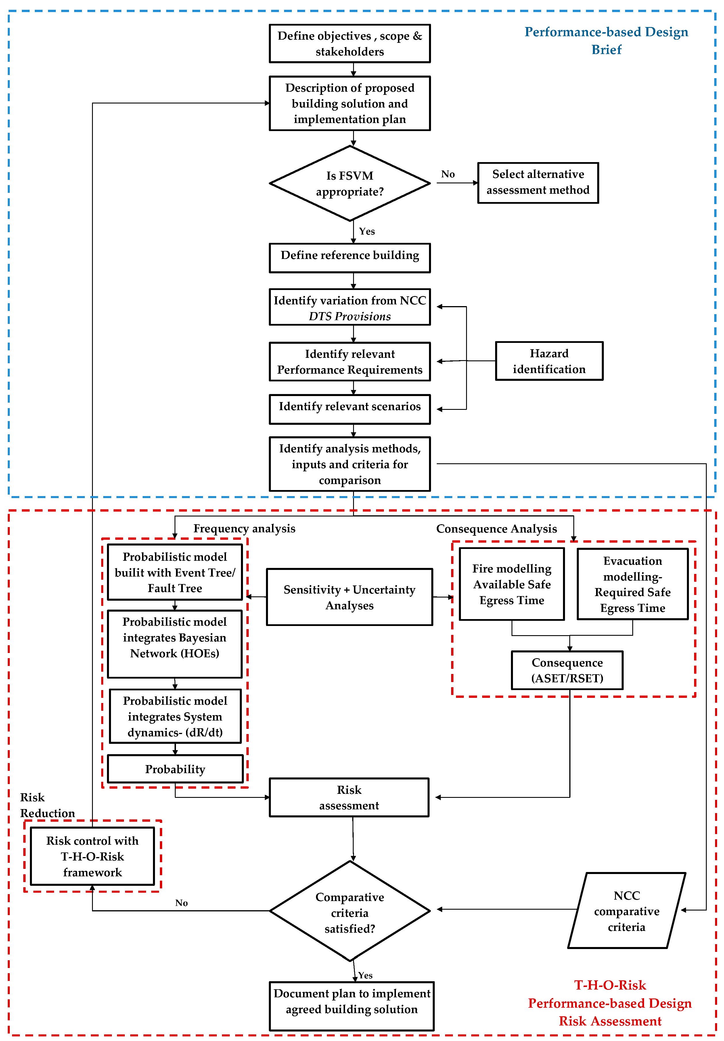
The Australian FSVM specifies twelve typical design scenarios for establishing if a building solution satisfies the relevant performance requirements. The proposed solution is then compared against a reference design which complies fully with the NCC Deemed-to-Satisfy (DTS) requirements. As the performance requirements are not quantified, the DTS building serves as a benchmark for acceptable safety level. The development of the FSVM process takes place in two different documents; a performance-based design brief (PBDB), which contains a description of all decisions of the stakeholders to perform the assessment, and a report which illustrates the execution and results from the risk assessment. To assess compliance with NCC, the required steps for completing the PBDB are shown in Figure 1 which enhances existing FSVM by incorporating T-H-O-Risk methodology.

Note that the developed T-H-O-Risk model is incorporated in the last step of the flowchart for comparison of technical, human and organizational risk levels of the performance building and reference DTS building. The choice of reference building should be based on an agreement with all the stakeholders and will have the following characteristics:

• Fully comply with the NCC DTS provisions;
• Comply with other relevant regulations;
• Have the same footprint, floor area and volume as the proposed building;
• Be of the same NCC classes as the proposed building;
• Have the same effective height;
• Have the same occupant load and occupant characteristics;
• Have the same fire load and design fire.

2.2. Methodology

The Australian FSVM provides a deterministic assessment of risk estimation in high-rise buildings. It provides standard design scenarios covering different fire safety aspects of a building. If the criteria fulfilled for these design scenarios are within certain thresholds, the design of building is considered safe. The limitations of this approach are that only technical factors are considered in the model and component reliability and failure rates are not accounted for in the framework. The T-H-O-Risk model improves on the existing FSVM by incorporating both technical and human errors into the simulations. Since HOEs are accounted for in this model, the T-H-O-risk model provides more accurate and realistic estimates of risk. The methodology develops a risk-based performance-based approach to generate alternate solutions, amongst which lower risk designs can be selected which enhances existing FSVM solutions while providing flexibility to fire safety engineers. In the next sections, the incorporation of the T-H-O-Risk model into the Australian framework is assessed.

2.3. FSVM

The FVSM requires several phases to be accomplished before conducting the risk analysis, among which the most relevant are the definition of the proposed building design and the corresponding DTS solution, the variations from the DTS solution and the identification of the relevant performance requirements. The FSVM presents twelve design scenarios that cover fire engineering design compliance on egress, active and passive systems, fire spread and fire brigade intervention and safety systems redundancy. Some or all of these design scenarios may be considered for the performance solutions, depending on the scope of the assessment and the desired fire safety level. The performance solution must be at least equivalent to that of the DTS solution. The description and analytical process of the design scenarios applicable to the fire engineering design of the case studies are presented in the following subsections. The fire engineering design is comprised of quantitative assessments utilising current fire and evacuation modelling and risk assessments tools.

2.4. T-H-O-Risk Framework

The PRA-based T-H-O-Risk methodology includes a set of sequentially linked tools and techniques. These are used to estimate probabilities and consequences for several fire scenarios and provide output in the form of both individual and societal risk. The process is described concisely here while the complete methodology can be found in our earlier papers [27,28,29]. Appendix A provides more details on the T-H-O-Risk methodology that incorporates ETA, FTA, Bayesian networks, system dynamics, and fire and evacuation modelling to determine available safe egress time (ASET) and required safe egress time (RSET). Briefly, the model involves the following steps:

• Calculation of the frequency of ignition: the calculation is based on [32]. The resulting value is then multiplied by the probability of a fire located in a sole-occupancy unit (SOU), in other words an apartment fire, or in the corridor (corridor fire).
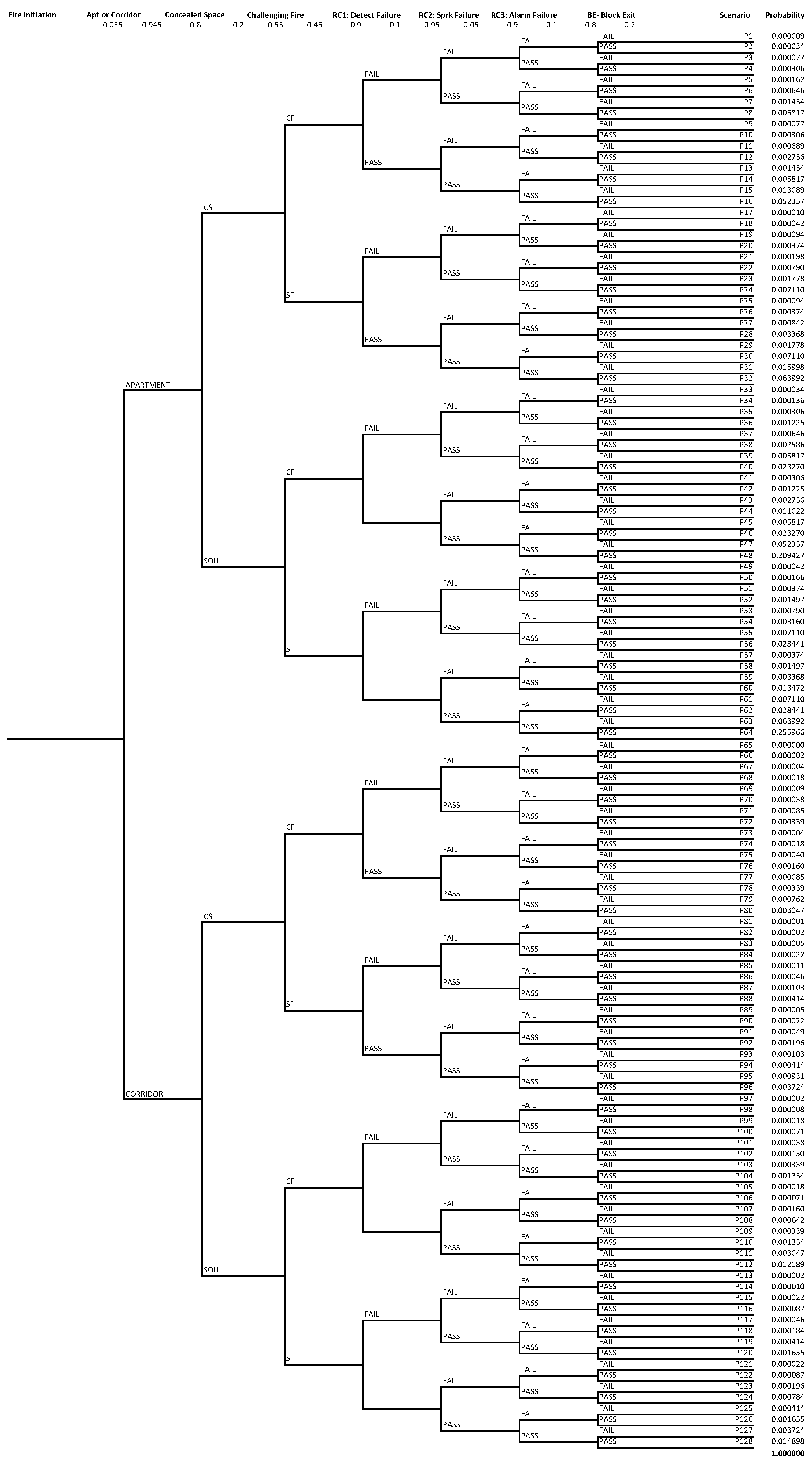
• Deployment of the accident scenarios and calculation of the associated probability using ETA: starting from the initiating event, the possible scenarios are derived by assuming a set of events that could or could not happen. The events are related to the effectiveness of the safety countermeasures (detection, notification, sprinkler, smoke management system) hat is linked to the type of fire (flaming or smouldering). FTA, a top-down failure analysis tool, is used to estimate the effectiveness of the safety measures.
• Calculation of the consequences for each scenario using ASET/RSET analysis: as described elsewhere, consequences are estimated by comparison of the ASET and the RSET. The first parameter is obtained from the B-Risk fire modelling simulation by determination of the time available before untenable conditions occur; the second is obtained as the sum of the time to complete different evacuation phases (detection, notification, pre-movement, and movement). Those times are derived partly from analytical calculations (hydraulic model), and partly via B-Risk simulation.
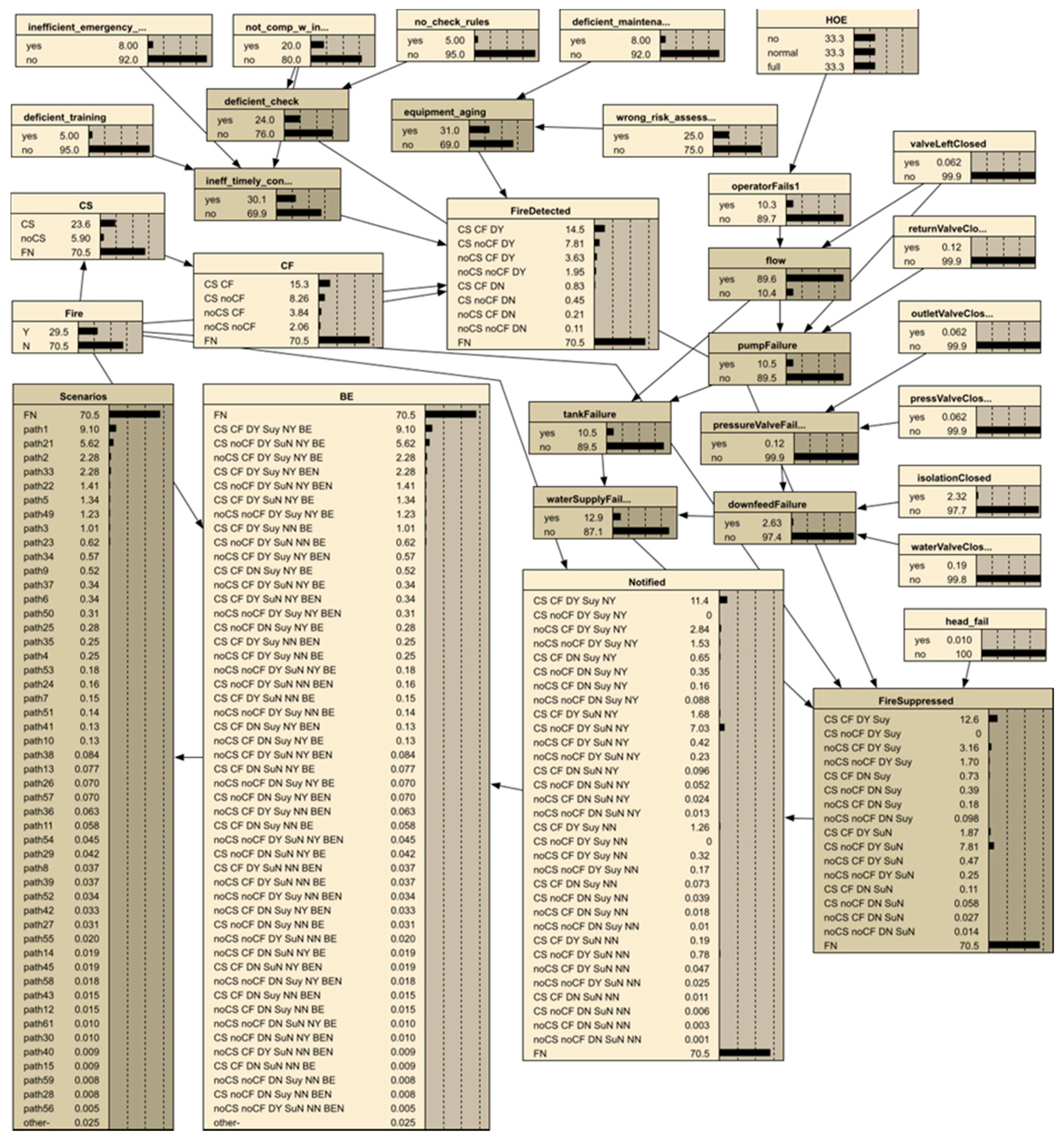
• Introduction of HOEs through a BN: a static evaluation of the effects of human and organisational failures is performed through a BN. The ET structure of the model is converted into the more flexible BN which allows the description of multiple relationships between variables.
• Calculation of the individual and societal risk for different contexts (level of organization): the impact on the risk of a good or bad safety organisation is investigated using two different indicators. The first indicator is a single risk value, the Expected Risk to Life (ERL), which expresses the risk in deaths/year*building; the second risk indicator, the SR is represented using the Frequency—Consequences (F-N) curves. F-N curves allow a comparison of the different solutions on Societal Risk which reflects average risk, in terms of death that a whole group of occupants is exposed to a fire scenario instead of looking at individual occupant. This second indicator is helpful in the decision-making process, introducing the possibility of adopting human-related countermeasures.
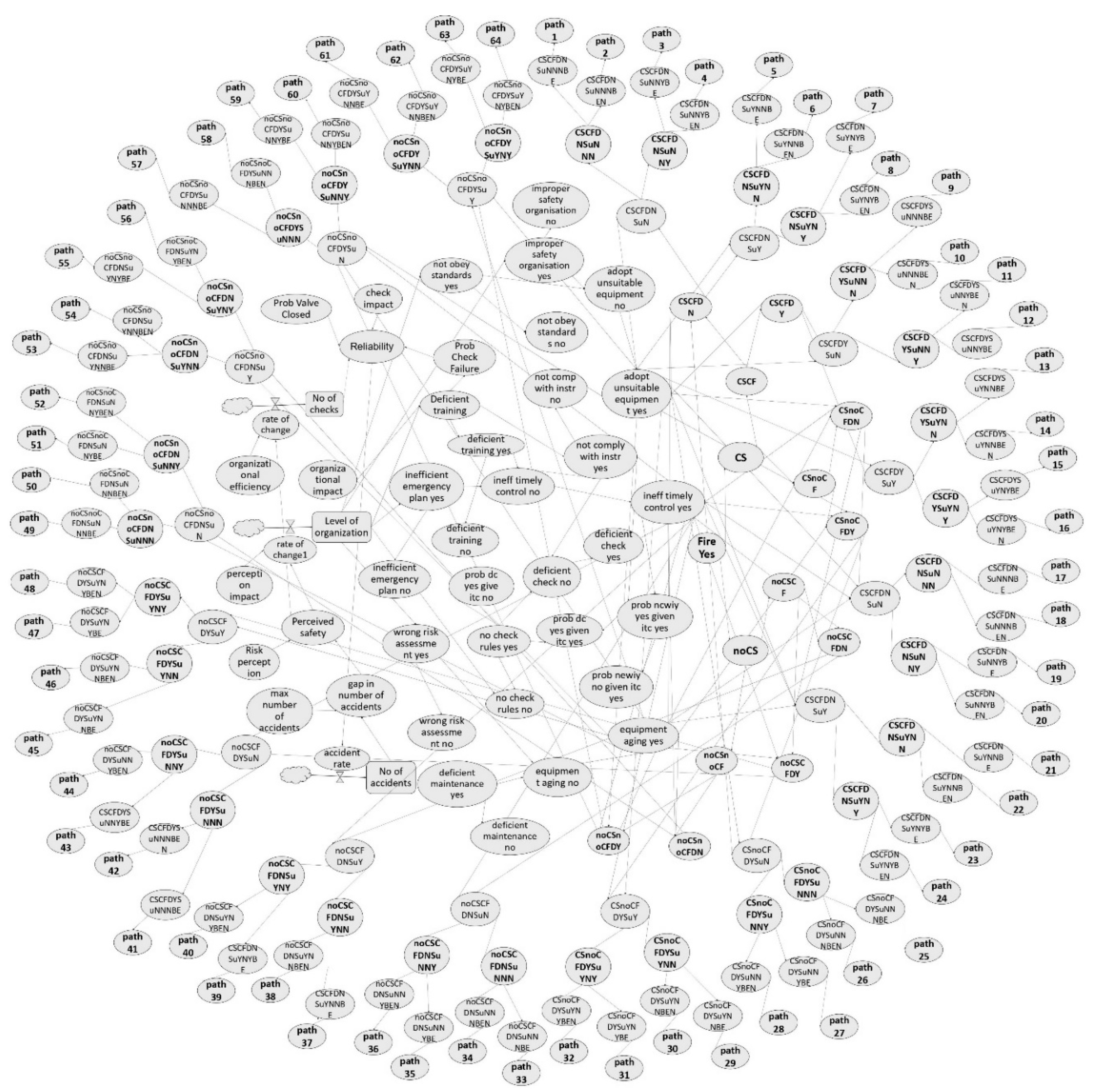
• Dynamic modelling of risk variations in the system using SD: to include future changes of the various components of a complex system, the evolution along its entire life cycle should be investigated. The analysis incorporating changes over time is performed with SD: each parameter of the system is checked along a period of ten years and hypotheses are made on the evolution of their values in relationships with all other parameters. A ‘societal’ loop is created which enables the modelling of HOEs in response to changes in the perception of the risk in the system.
• Calculation of the time—risk curve for the entire lifecycle of the building.
• Sensitivity and uncertainty analyses using a Monte Carlo approach. Uncertainties in point estimates of ERL values are propagated through probability distributions with Monte Carlo simulations while a family of F-N curves and confidence intervals propagate epistemic uncertainty on SRs. Sensitivity and uncertainty analyses are also performed on key variables in the SD model to assess model robustness and to explore how uncertainty affects the assessment of different safety systems and reliability of model outputs.

2.5. Sensitivity and Uncertainty Analysis

A sensitivity analysis is conducted to determine the most influential HOE variables on the model outputs while uncertainty analysis is used to assess how much uncertainty is associated with these influential variables. The purpose of these analyses is to determine the HOE-related influence on risk. A Monte Carlo approach is adopted to perform the analysis; a sampling is generated from the probability distributions and the output of the model is determined and represented in different graphs. The number of samples has been fixed to 1000 samples for an acceptable level of confidence. The following steps are performed for the sensitivity and uncertainty analyses.

First, the responsive parameters are identified. Second, for each of the responsive human and organizational parameters, a univariate analysis is performed to assess the sensitivity of the target variables to characterize which variables are more sensitive to the organisational response. The quantification of the uncertainty allows for both comparative and absolute risk analysis; when using the comparative approach, it ensures that the point value of the individual risk of the performance solution is below that of the DTS solution even if HOE-related errors are taken into account for both designs. It can be possible, in theory, that the first of the two solutions is more prone to be influenced by human factors than the second, or vice versa. For the performance solution to be approved, it is therefore important to find the upper and lower limits for both the risk values and verify that the upper bound value of the performance solution is below the lower bound solution of the DTS solution. When risk evaluation is conducted in absolute terms, the oscillations of the risk value should never trigger the reference value. The uncertainty analysis allows a deeper understanding of the propagation of HOEs through a risk model for high-rise buildings subject to fire.

In the sensitivity analysis, a simple mono-dimensional analysis is conducted based on point values. The HOEs (deficient training, inefficient emergency plan, not comply with instruction, no check rules, deficient maintenance, wrong risk assessment, not obey standard, improper safety organisation) are attributed with a probability distribution built based on a three-point estimation method. In a multivariate analysis, the sensitivity is represented in a tornado graph showing the variables with major impacts on the final risk value. When considering a single parameter, the relative amplitude of the variation of the global risk value is compared to the relative amplitude of the variation of the parameter value (sensitivity). Moreover, the model is used to determine the amplitude of the risk variations in cumulative terms. This in fact can be beneficial for more detailed analysis of the risk in relationship to the entire society.

Sensitivity analysis is further conducted on key variables in the SD model to assess model robustness and to explore how uncertainty affects the assessment of different safety systems and reliability of model outputs. Once the sensitive parameters for each HOE variable have been identified in the previous steps, a Monte Carlo simulation is carried out. The linkage of these variables to their parent nodes is the focus of this analysis. The causal loop in the SD model consists of all the variable and their interactions with each other including feedback loops and time delays. Stocks are accumulations in the system used to represent variables that change with time and flows are entities that control these stocks. The behaviour of the HOE variables depends on the parent variables connected to them in the causal loop and delays are to be expected in the response to safety issues due to feedback loops occurring over a period of time. Therefore, if the system is observed on a wider time scale over ten years, oscillations in the final output are possible, generating phases during which the risk could vary greatly with respect to the static value. To develop a better understanding of those dynamic phenomena, parent nodes, are varied and the corresponding variation in the value of the target variables (children nodes) is investigated.

The propagation of uncertainty is modelled using the Monte Carlo technique applied to the ET to calculate uncertainty related to the probability of accidents (ordinate of the F-N curve). The same approach is then used to model the uncertainty related to the number of deaths, in the abscissa of the F-N curve. This allows an expansion of the single F-N curve to a family of curves that can be considered representative of the effective SR. In this way, the confidence of the model output can be increased.

3. Case Studies

Four cases have been selected for this study. Three of the cases are taken from our previous studies [27,28,29]. The fourth case is an ABCB FSVM Handbook reference case study. The ABCB case will enable us to benchmark against the other three selected cases.

3.1. Objectives and Performance Requirements

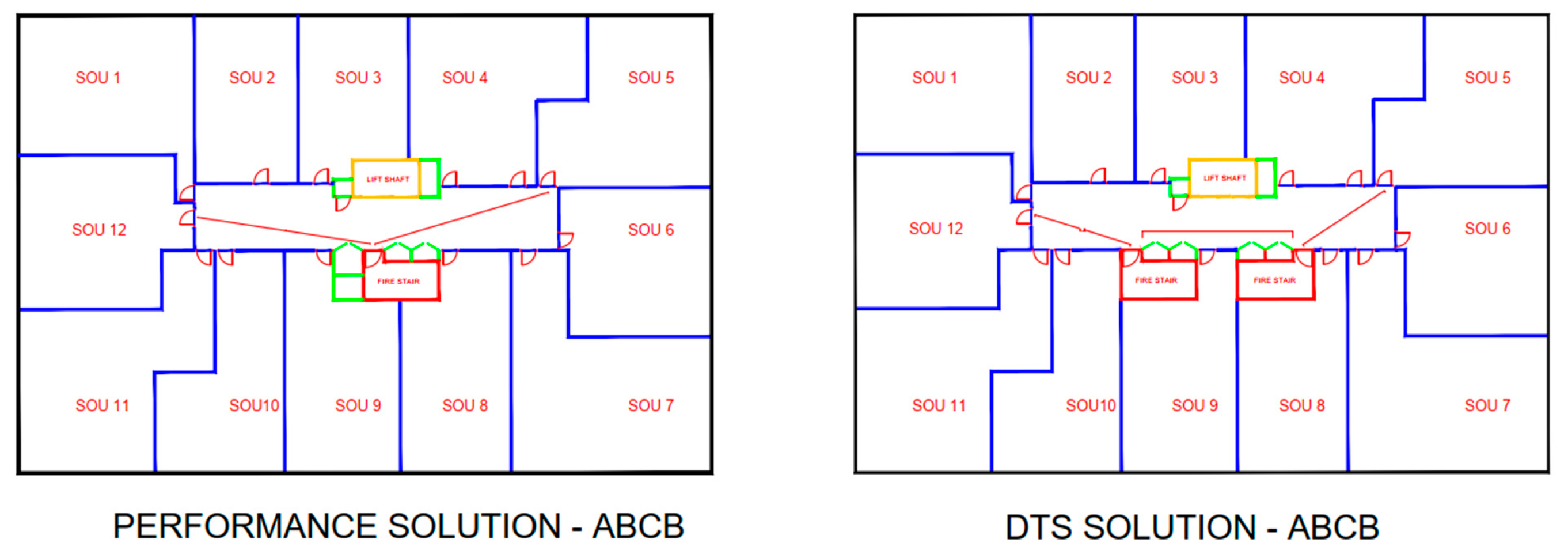
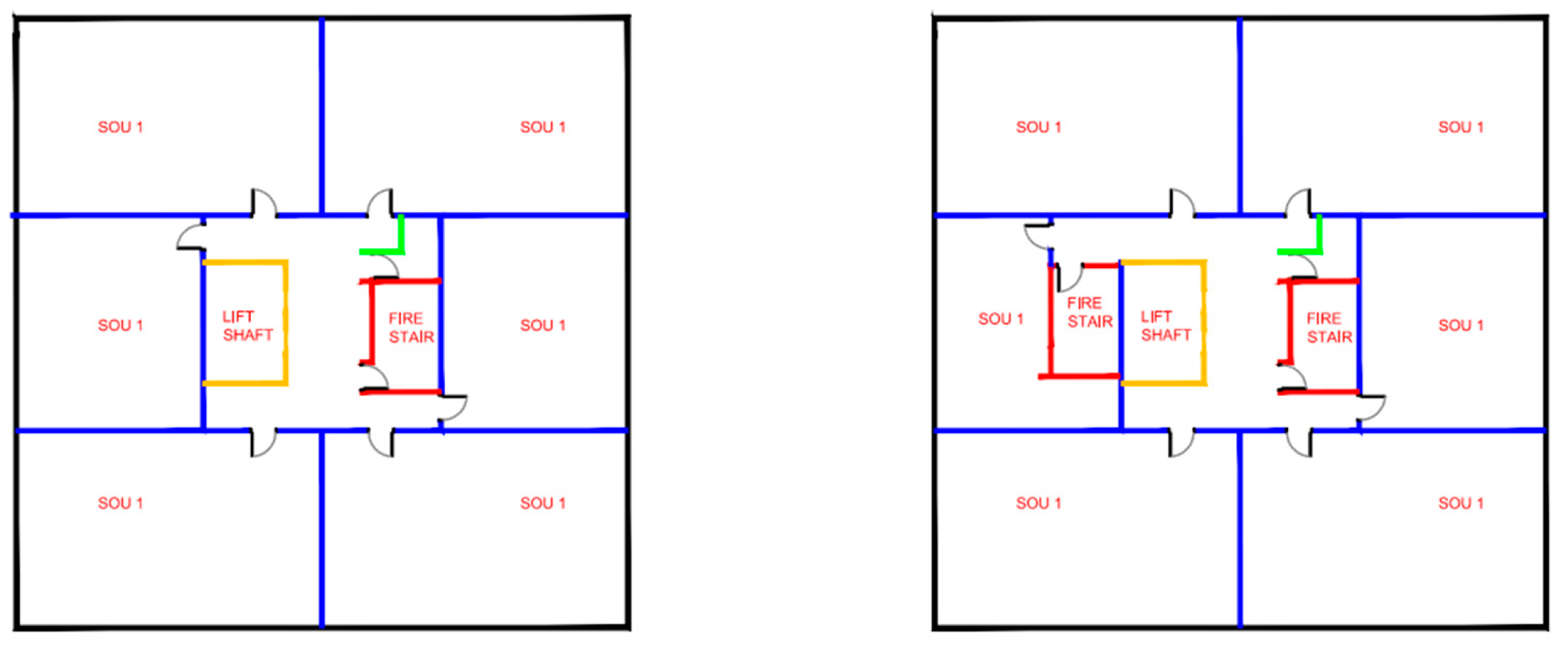
The first proposed design (Case 1—ABCB) is a 20-storey residential occupancy building with twelve units per floor. The performance solution provides a single fire stair for each floor while the DTS solution provides a double exit stair in compliance with the requirements from NCC. Both designs are taken from the FSVM Handbook and are shown in Figure 2.

Table 1. Characteristics of Case #1- Australian Building Codes Board (ABCB) Deemed-to-Satisfy (DTS) and Performance solutions.

Building Characteristics	ABCB DTS	ABCB Performance
Occupants per floor	36	36
Number of floors	20	20
Floorplate area (m2)	702	702
Number of units per floor	12	12

summarizes the main characteristics and differences between the two solutions. When examining the floor plan of a single floor, space saving by using a single fire stair does not appear to be significant, however the space savings over twenty floors can be quite significant. Additionally, construction cost savings from not constructing the second stair compartment is also substantial.

The comparison of the two designs shows that the performance requirement that is not met by the proposed design is the DP6 (Paths of Travel to Exits) requirement. The building is classified as a Class 2 building according to the NCC, Volume 1. Given the height of more than 25 m, the DTS design shall have at least two exits from each storey. The second element of non-compliance for the performance solution is the exit travel distance (D1.4) [21]. The DTS condition requires that the ‘entrance doorway of any sole-occupancy unit must be not more than 6 m from an exit or from a point from which travel in different directions to two exits is available’. Moreover, the distance between alternative exits must be not less than 9 m and not more than 45 m.

These DTS requirements are expected to be compensated by introducing other safety measures that are not contemplated in the DTS solution. The method used to compare the risk in the two buildings is the T-H-O-Risk method. The output from the application of the method to the two solutions will generate two risk values that will be compared to assess the level of safety of the performance solution. Using the FSVM, a selection of the design scenarios can be made based on the performance requirement that is violated (using Table 1.2 of the Handbook for FSVM [21] as a guide). Consequently, the design scenarios that need to be modelled are as follows:

• BE—Blocked Exit, a fire blocks the evacuation route; it is necessary to demonstrate through ASET/RSET and ERL analysis that the level of safety is at least equivalent to the DTS provisions.
• CS—Concealed Space, a fire starts in a concealed space that can spread and harm several people in a room. The solution might include fire suppression or automatic detection.
• SF—Smouldering Fire, a fire is smouldering close to a sleeping area. The solution may provide a detection and alarm system.
• IS—Internal Surfaces, interior surfaces are exposed to a growing fire that potentially endangers occupants.
• CF—Challenging Fire, the worst credible fire in an occupied space.
• RC—Robustness Check, failure of a critical part of the fire safety system will not result in the design not meeting objectives of the NCC (modified ASET/RSET analysis to demonstrate that the remaining floors or fire compartments are robust).

For each of the fire scenarios, a fire modelling simulation based on fast t-squared fire (α = 0.0469) up to flashover will be performed to determine ASET based on tenability limits. The same approach is used for the other three cases (Figure 3, Figure 4 and Figure 5), with characteristics shown in

Table 2. Characteristics of the building case studies.

Building	Case #2		Case #3		Case #4
Characteristics	Performance	DTS	Performance	DTS	Performance	DTS
Occupants per floor	24	24	54	54	58	58
Number of floors	24	24	23	23	21	21
Floorplate area (m2)	484	484	1099	1099	1343	1343
Number of units/floor	6	6	15	15	20	20

.

In Case #2, as shown in Figure 3 the performance solution has only a single exit stair similar to Case #1, while for Cases #3 and #4 (Figure 4 and Figure 5, respectively); the performance solutions deviate from the required 6 m dead end travel distance. As described in [29], Case#2 is located in UK and Cases #3 and #4 are in Australia—all in a temperate climate.

3.2. Probability Analysis of Human and Organizational Errors

In addition to technical factors, a review and analysis of the literature is performed to obtain probabilities and frequencies of the important HOEs. These probabilities and frequencies are assigned to initiating events and basic events in the model to carry out a quantitative analysis of the frequency of occurrence. The Fussel-Vesely method [33] is used to determine the important HOEs as described in Appendix A.

3.3. Event and Fault Tree

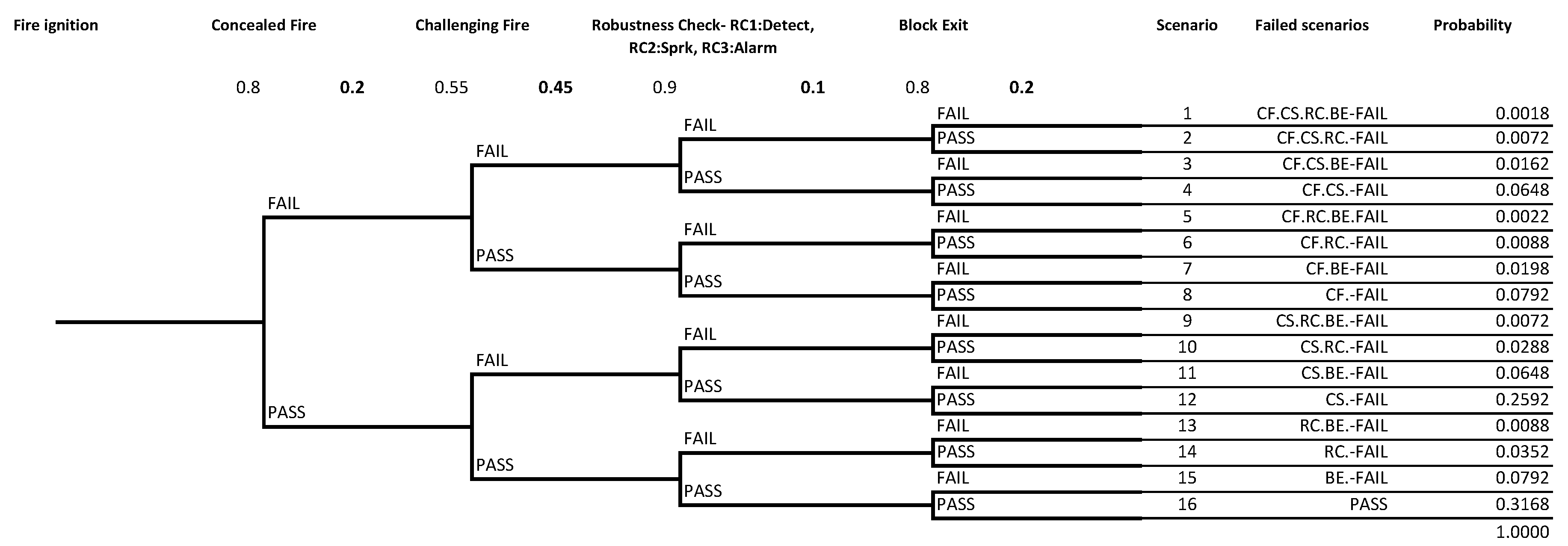
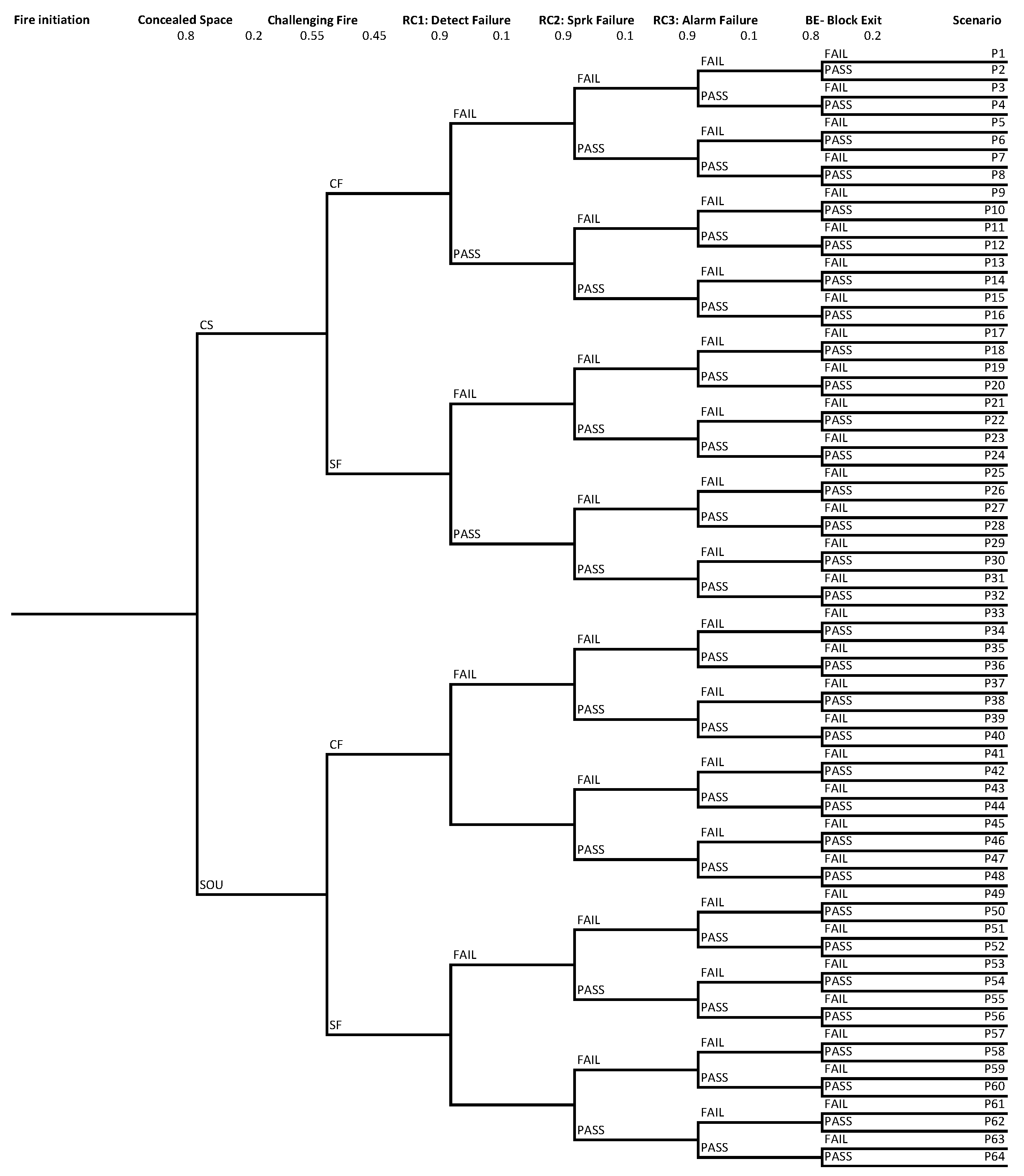
The ETA uses a logical technique to examine the failure and success of technical risks emanating from an event. The initial and subsequent events are assigned probabilities and possible outcomes contributing to computations of expected number of consequences. Typical fire safety sub-systems used in high rise buildings are fire detection systems, emergency notification systems, fire suppression systems, interior fire barriers, floor compartmentation (vertical barriers) and building egress systems. The ET incorporates all fire safety sub-systems expected to be present within the high-rise residential buildings as they relate to occupant evacuation as well as the relevant FSVM design scenarios that are applicable to the case studies as follows: (i) CS—Concealed Space (ii) CF—Challenging Fire (iii) BE—Blocked Exit and (iv) Robustness Checks where RC1 is failure of detection, RC2 is failure of sprinklers and RC3 is failure of building alarm. Events are assumed to be independent of each other. The fire safety sub-systems in high-rise buildings are often provided with redundancies to avoid a single point failure. An efficient fire safety system will increase ASET and reduce RSET. The ET helps in identifying the critical sub-system path of fire safety that leads to better mitigation measures.

A typical ET is shown in Figure 6. After the fire is initiated, the first branch is whether fire is in a concealed space or SOU/corridor with a probability of 0.2 and 0.8, respectively. In the next event, this fire can develop into a challenging fire (>5 MW) or a smouldering fire with a probability of 0.45 and 0.55, respectively. Further in the next event, failure of fire detection occurs with a probability of 0.1. Next in the chain comes the sprinkler system with a failure probability of 0.10. A building alarm failure occurs with a probability of 0.1. The probability of the next event, which is blocking of an exit, has a failure probability of 0.2. The failure probabilities assumed are slightly conservative compared to the literature (Appendix B,

Table A4. Failure probabilities of technical risks implemented in Event Tree analysis.

Safety System Failure	Critical Component	Low	Expected	High	Reference
Challenging Fire		0.25	0.35	0.45	Hall [54]
Emergency Exit is Blocked	Human error	0.15	0.20	0.25	Magnusson et al. [55]
Fire in Concealed Space	Non-combustible partition ceiling/wall	0.15	0.20	0.25	N.A.
Sprinkler system	Main valve shut off, Human errors	0.02	0.05	0.15	Moinuddin & Thomas [43]
Smoke detection	Poor maintenance	0.05	0.10	0.15	Bukowski [56]
Alarm system	Shut-off after maintenance	0.05	0.10	0.15	PD7974−7 [6]
Manual detection	Human errors	0.30	0.48	0.60	Holborn et al. [57]
Smoke Control/Mechanical ventilation	Fire damper failure	0.20	0.30	0.50	Zhao [58]
Smoke barrier	Door seal failure	0.05	0.20	0.50	PD7974−7 [6]
Fire department response	Human and organizational errors	0.02	0.05	0.30	USFA [59]
Management strategy	Human errors	0.05	0.15	0.30	Sabapathy et al. [40]

) and so will likely result in slightly higher, yet acceptable ERL values. In the worst credible case, the fire ignition occurs in a concealed space, developed into a full CF, the sprinkler system fails (robustness check) and the emergency exit is blocked (BE). In the best case scenario, the fire does not occur in a concealed space, but in the living room of the SOU, does not develop into a full CF, there is no failure in sprinkler or alarm or detection and the emergency exit is not blocked.

The frequency and number of fatalities are also shown in Figure 6. The two most critical events resulting into maximum number of deaths are CF and sprinkler failure. That is, if fire develops into a CF and sprinkler fails, it leads to maximum fatalities. A fire will not be controlled if the fire sprinkler system is not functioning properly. When the sprinkler system is activated, fire growth is controlled or extinguished. If the sprinkler system fails, the fire continues to grow until untenable conditions occur. The negative effects of a fire spreading throughout the building are directly related to the failure of each sub-system. Systems performing as intended will elongate the ASET giving occupants more time to reach safety. The number of consequences is dependent on the reliability of the detection, suppression, notification, containment, robustness and egress sub-system systems. (The failure probabilities for sub-systems assumed in this study are provided in Appendix B, Table A4)

The first node of the ET is the ignition frequency; using the Barrois model [32] equation as:

$${\mathrm{P}}_1\left(\mathrm{A}\right)={\mathrm{c}}_1{\mathrm{A}}^{\mathrm{r} }+{\mathrm{c}}_2{\mathrm{A}}^{\mathrm{s}}$$

(1)

where P₁(A) is the ignition frequency of a building with floor area A/year, c₁, c₂, s and r constants based on [32] (refer Appendix A).

3.4. Bayesian Network

As the FT/ET can only handle technical factors primarily in Boolean form, HOEs are introduced into the model through BNs. The FT/ET used to determine the probabilities for each possible outcome of the fire event is mapped into a BN for the incorporation of HOEs.

The inclusion of the FT/ET in the BN is shown in Figure A2 and described in Appendix A.

3.5. System Dynamics

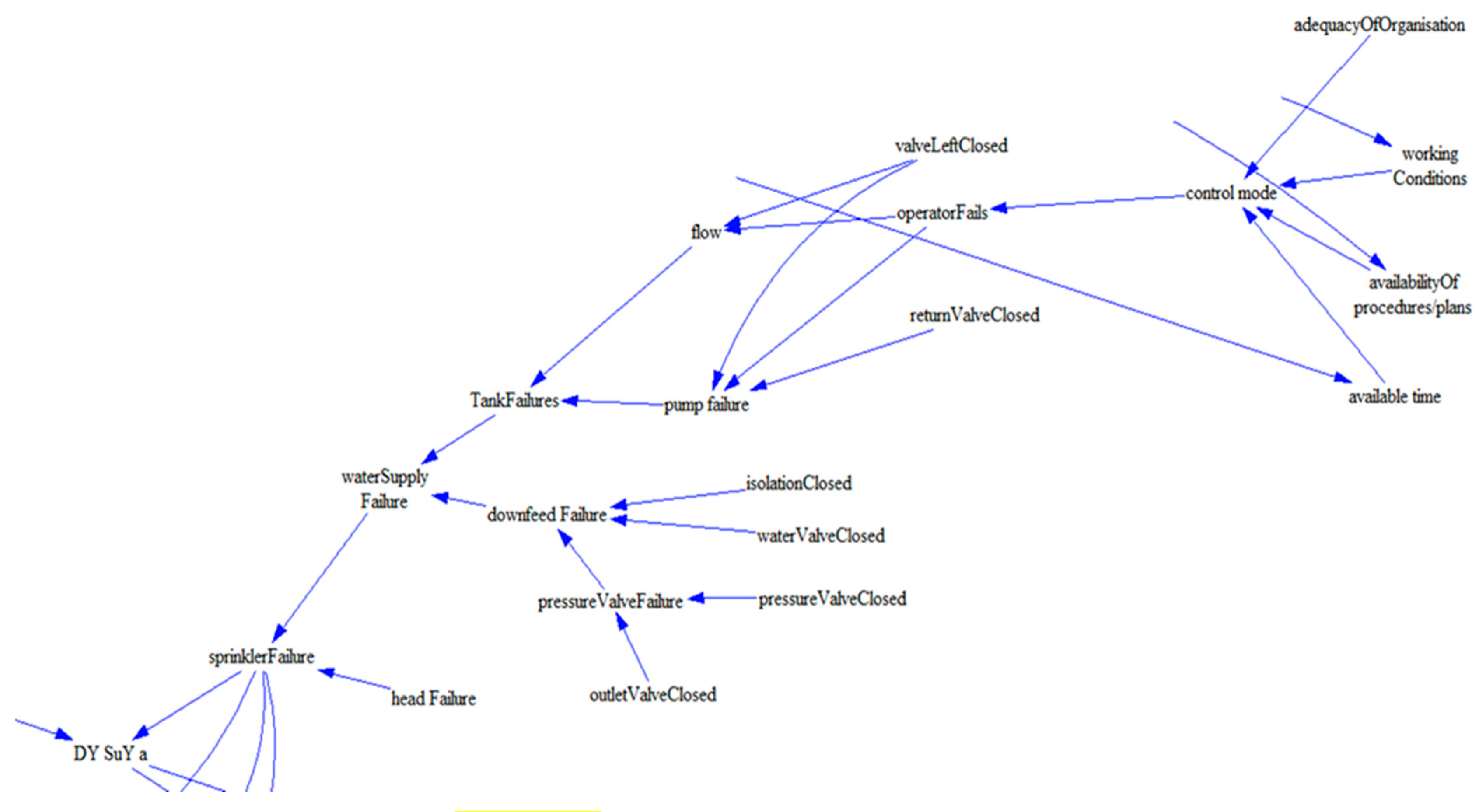
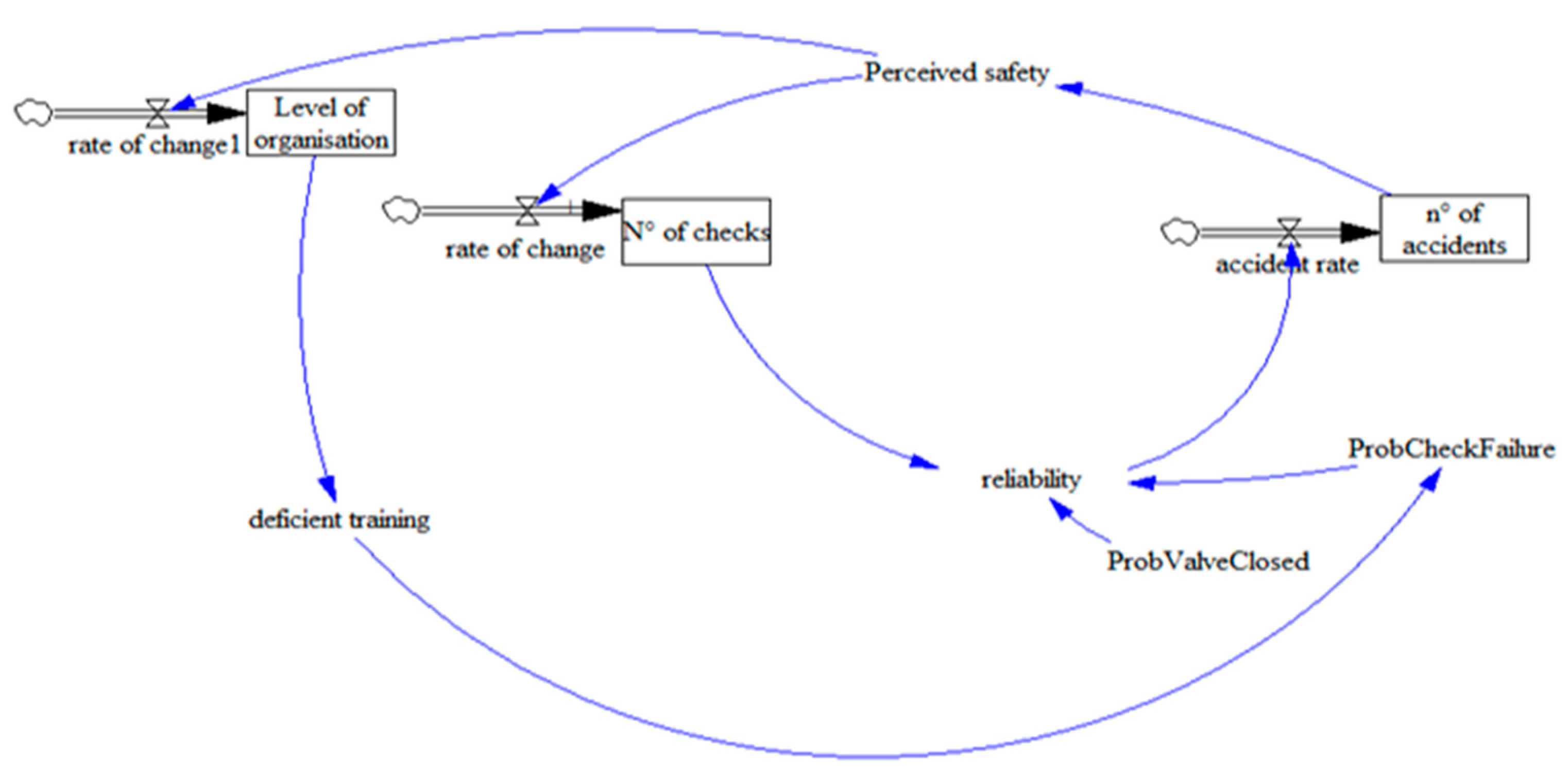
System dynamics modelling is used to obtain time-varying probabilities which allows for the representation of feedback loops and delays and to allow for the estimation of risk variations over time of the system. The SD model is shown in Figure A5 and described in Appendix A.

3.6. Consequence Analysis & Design Scenarios

To estimate the consequences, different characteristics of the various fires are analyzed. This includes exits blocked by a fire, fire in concealed spaces, smouldering fires, challenging fires and a robustness check. These characteristics are described in further detail below.

The FSVM associates each performance requirement that has been individuated with the hazard identification process to a certain number of design scenarios to be tested (see Table 1.2 of FSVM Handbook [21]). In the specific case, the performance requirement is the DP6 (Paths of Travel to Exits), which requires only 4 design scenarios to be modeled (BE, CS, CF, RC). The SF scenario in our model is assumed to produce no casualties and has been not modelled. The RC scenario is required to be one where a safety measure (e.g., detection, sprinkler, alarm) is not working as expected; in the T-H-O-Risk model the RC event is included in the analysis of the DTS and performance solution. The details of the numerical experiments are shown in

Table 3. Table of experiments for FSVM design scenarios.

Design Scenario	Numerical Experiment #	Solution	Fire Spread
Fire blocks evacuation route	BE1	Performance	Yes
	BE2	Performance	No
	BE3	DTS	Yes
	BE4	DTS	No
Fire starts in concealed space	CS1	Performance	Yes
	CS2	Performance	No
	CS3	DTS	Yes
	CS4	DTS	No
Robustness Check	RC1	Performance	Yes
	RC2	Performance	No
	RC3	DTS	Yes
	RC4	DTS	No
Challenging fire	CF1	Performance	Yes
	CF2	Performance	No
	CF3	DTS	Yes
	CF4	DTS	No
Fire in a normally unoccupied room threatens occupants of other rooms	UT	Not required
Smouldering fire	SF	Not required
Internal surfaces	IS	Not required
Structural stability and other properties	SS	Not required
Horizontal fire spread	HS	Not required
Vertical fire spread involving cladding or arrangement of openings in walls	VS	Not required
Fire brigade intervention	FI	Not required
Unexpected catastrophic failure	UF	Not required

and the simulations yield the results as presented in

Table 4. Results from B-Risk simulation for case #1 Blocked Exit fire.

Tenability Criteria	Sole Occupant Unit	Corridor	Stairway
Upper Layer temperature	n	n	150 s
Lower layer temperature	n	n	90 s
Visibility	240 s	150 s	59 s
FED thermal	n	n	135 s
FED asphyxiant	n	n	1011 s

.

3.7. Fire Safety Verification Methods—Applicable Design Scenarios

3.7.1. Exit Blocked by a Fire

The fire in a blocked exit scenario is assumed to occur in the stairway where a low fire load is expected. Hence, it can be estimated that a fire has a peak heat release rate (HRR) of 2500 kW. The DTS building shows an individual risk indicator largely greater than the performance solution, hence for this scenario the performance design is verified.

3.7.2. Concealed Space

In this design scenario, the fire starts in a concealed space between two rooms. This fire can be electrical in origin and develop behind a curtain or within a wall with a slow-growth fire (α = 0.0117 kW/s²). It is assumed that the initial fire is in the bedroom and the fire develops to engulf the mattresses (data from fire test from mattresses re-reported in SFPE Handbook [8] to be around 2 MW).

3.7.3. Smouldering Fire

The assumption in the model is that the smouldering fire is readily cured by occupants and extinguished. Hence, no simulation is determined for this scenario.

3.7.4. Internal Surfaces

The design scenario of a fire igniting internal surfaces of a compartment can become risky for occupants. The fire is then determined to be a fast-growing fire (time to growth is 150 s, so α = 0.0469 kW/s²). This scenario affects fire growth and fuel load in a fire compartment and is addressed in the consequence modelling.

3.7.5. Challenging Fire

The worst-case fire is a fire that develops into a flashover and involves all combustible materials in a dwelling. The fire could be modelled as a fast-growth fire (NFPA 72 [34], 150 s) with a peak of 10 MW. The fire burns at 10 MW HRR until the end of the simulation.

3.7.6. Robustness Check

This scenario tests the robustness of the design by assuming that a key component of the fire safety system fails. The required outcome is that if a single fire safety system fails, the robustness of the building will prevent disproportionate spread of fire (e.g., by showing that ASET/RSET for the remaining fire compartments is satisfied).

3.8. PRA—ASET/RSET Analysis

To determine the associated risk, is necessary to calculate the expected consequences, expressed in casualties. The determination of the casualties is the result of an ASET/RSET analysis and is based on a computer simulation of the fire scenarios. To reduce the burden of the simulation work, the number of simulated scenarios can be reduced by making some assumptions:

• A smouldering fire yields no casualties as the fire is limited in size and generally its extinction is performed by occupants before the fire develops into flashover.
• When suppression systems work as expected, the fire is controlled, and there are no victims.
• When the egress protection system is working as expected, untenable conditions do not arise in the corridor, hence the ASET is infinite and there are no victims (all scenarios identified with an odd number).

The scenario where fire spreads is modelled with the following assumptions:

• The fire starts in the corridor/stairs; exit doors are not closed due to door blockade or due to failure of the self-closing mechanism. Smoke leakage through SOU doors.
• The fire starts in SOU; SOU doors remain open after the people have left the apartment (the self-closing mechanism is not working). Exit doors remain open due to door blockade or due to the failure of the self-closing mechanism.

With these assumptions, there are 8 scenarios for each fire location, resulting in a total of 16 scenarios for each design. The fire modelling simulations are performed using the B-Risk [35] fire modelling software as used in previous studies [27,28,29] and requires two different scenarios for each location, one with the fire spreading into common parts and the second with fire restricted to the area of fire origin. The application of FSVM implies that the selection of fire scenarios is based on the performance requirements that have been selected in the hazard identification phase (see Chapter 8 from the FSVM Handbook [21]).

The simulation output consists of a set of ASET values, each associated with a different scenario. The B-Risk software calculates in each time step the enclosure conditions in terms of five different tenability parameters: upper layer temperature below 200 °C, lower layer temperature below 60 °C, FED for asphyxiant gases below 0.3, FED for thermal effects below 0.3, and visibility above 10 m. The first value that triggers the above value determines the ASET, except for visibility, which is excluded in the room of fire origin and in the corridor. In these spaces, it is assumed that the occupants have familiarity with the exit route, so the visibility is not relevant. With stairs, visibility is an impeding factor as the occupants are assumed to be unfamiliar with the environment. B-Risk estimates the detection time by simulating the response time of smoke detectors or heat detectors. In one such simulation, detection time was computed as 187 s and 107 s for SOU and corridor compartments, respectively.

4. Analysis

4.1. Verification Method Incorporating T-H-O-Risk to Compare ERL and HOEs

The application of the methodology shows that the level of risk of the performance solution is lower than that of the DTS solution, as required by FSVM for the relevant fire scenarios.

Table 5. ERL results of design scenarios for Case #1 to #4 (DTS, Performance, HOE (human and organizational errors)).

Design	Case #1	Case #2	Case #3	Case #4
DTS	3.21 × 10−5	4.02 × 10−5	2.64 × 10−5	3.98 × 10−5
Performance	3.03 × 10−5	3.91 × 10−5	2.18 × 10−5	2.98 × 10−5
Performance HOE	4.36 × 10−5	4.55 × 10−5	3.14 × 10−5	4.27 × 10−5

presents the ERL results of the design scenarios for the DTS solution, the performance solution and the performance solution with HOEs.

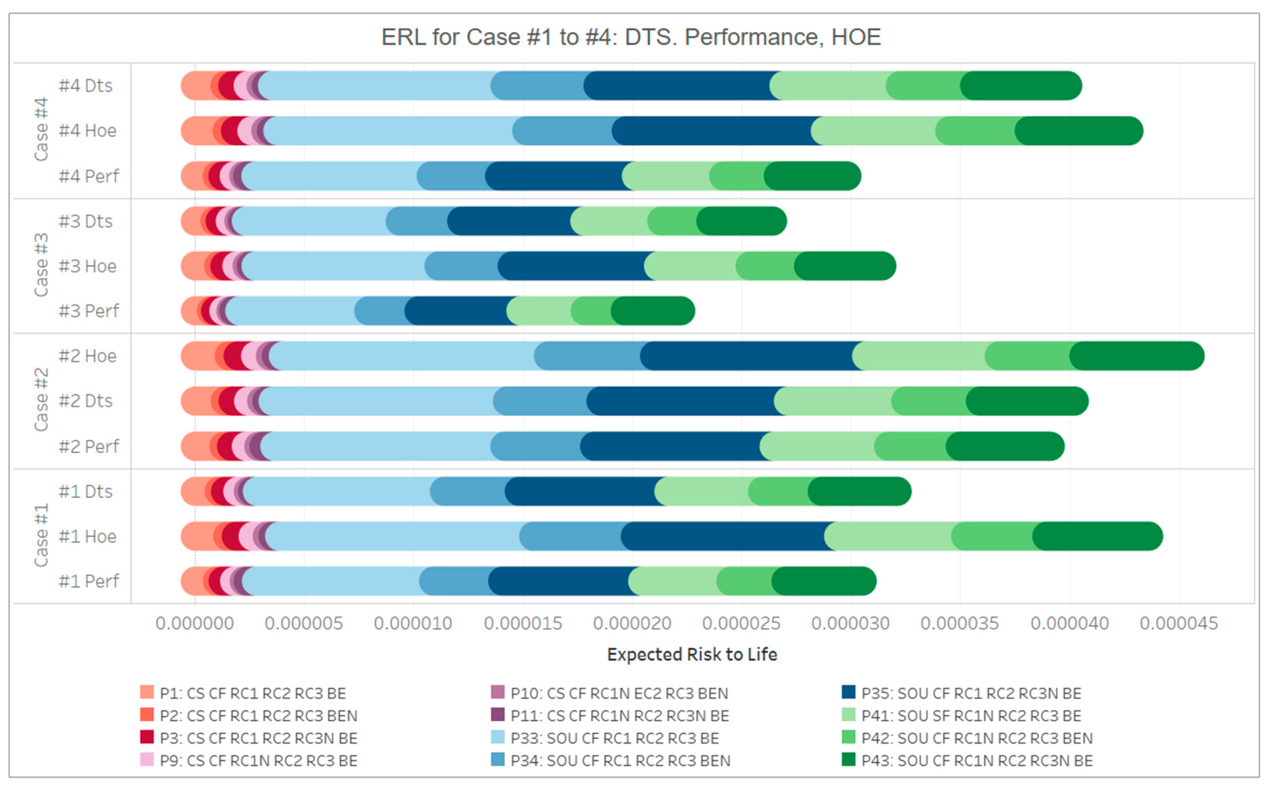
Figure 7 shows the ERL of the various scenarios in which consequences occur. Results of the T-H-O-Risk analysis indicate that the influence of HOEs is significant for all cases. A fire initiating in a SOU (P33) has a significantly higher ERL, i.e., 7.8 times higher than the fire initiating in a concealed space (P1). P33 has the highest risk as the flaming fire occurs in the bedroom of the SOU where all safety systems fail. Moreover, when all the fire safety strategies including fire detection, alarm, sprinkler, and emergency doors fail, the probability of failure is increased substantially. However, if at least one of the fire safety systems is successful, the probability of failure is considerably reduced. Scenarios P2 & P3 and P34 & P35 indicate that a blocked exit results in a higher ERL than building alarm failure.

It is evident from the figure that there are severe consequences in all scenarios where a challenging fire occurs while sprinklers also fail. When the sprinkler system fails, the role of the emergency exit door becomes very important. On the contrary, when the sprinkler system is activated, the emergency doors will be less important, and no fatalities are anticipated, hence showing that the sprinklers are critical to helping occupants to evacuate safely. The alarm system is another important safety measure. As shown in Figure 7, the probability of failure is significantly increased if the alarm system fails. When the four case studies are compared with each other, the results in Figure 7 indicate that the ERL values in Case #3 for different scenarios that consider HOEs are the lowest while for Cases #1 and #4, the values fall into a similar range. Case #3 has a double-loaded straight corridor configuration with full-height window openings at either end which results in elongated ASET conditions. Case #2 has a higher ERL on account of the sole stairway for performance and HOE solutions and low tenability due to the small corridor area filling up with smoke rapidly. More results for the four cases indicating similar patterns are discussed later in Section 4.2.2.

4.2. Sensitivity and Uncertainty Analyses of HOE Variables and ERL

In this section, a sensitivity analysis is carried out for the main HOE variables to rank them from the most influencing to the least from a risk perspective. The most influencing variables are then associated with a probability distribution and quantification of uncertainties related to design variables are examined. T-H-O-Risk is used as a verification method to compare HOEs in the various design scenarios. This is followed by F-N curve assessment where uncertainties in SR due to HOEs are propagated as confidence-level-based SR followed by risk over time analysis in the SD model. Lastly, the T-H-O-Risk model is validated against the risk data obtained from the literature for high-rise building fires.

4.2.1. Sensitivity Analysis of HOE Variables and ERL

Different weights are used for different performance shaping factors (PSFs) in the analysis. The most influencing HOE variables are identified from the analysis. For each test case, ERL values and variations are estimated using the Monte Carlo approach. It is to be noted that the ERL values are necessarily point estimates, where the probabilities of events occurring do not take uncertainty into account. The uncertainty inherent in point estimates of HOEs can be considered by estimating a range or distribution in which the probabilities lie (various distributions are described in Appendix B,

Table A5. Types of distributions.

Distribution	Graph	Probability Density Function	Properties	Framework
Uniform		$f\left(x\right)=\frac{1}{max-min}$	Close-ended with same probability	Same likelihood of either overestimating or underestimating (+/− 10%)
Triangular		$f\left(x\right)=\frac{2 \left(x-\min \right)}{\left(mode-\min \right)\left(\max -\min \right)}$ $if min\le x\le mode$   $f\left(x\right)=\frac{2 \left(max-\mathrm{x}\right)}{\left(max-\min \right)\left(\max -\mathrm{mode}\right)}$ $if mode<x\le max$	Close-ended With possible skewness	Possible under-estimation of ML is [−10%; ML: +50%
Beta		$f\left(x\right)=\frac{{\left(x\right)}^{\alpha -1}{\left(1-x\right)}^{\beta -1}}{B\left(\alpha ,\beta \right)}$   $\mathrm{Where} B\left(\alpha ,\beta \right) \mathrm{is} \mathrm{a} \mathrm{Beta} \mathrm{funtion}$	Close-ended with possible skewness	Possible under-estimation of ML is [−10%; ML: +50%
Normal		$f\left(x\right)=\frac{1}{\sqrt{2\pi {\sigma }^2}}exp\left(-\frac{{\left(x-\mu \right)}^2}{2{\sigma }^2}\right)$	Close-ended With no skewness	The most likely value is set to first-year impact, std. dev. is set to 15%
Gamma		$f\left(x\right)=\frac{{\beta }^{-\alpha }{x}^{\alpha -1}exp\left(-\frac{x}{\beta }\right)}{\mathsf{\Gamma }\left(\alpha \right)}$	Semi-close-ended Possible right skewness	k-value setting is 5, calculated based on mean from Lichtenberg [−25%; ML: +100%]

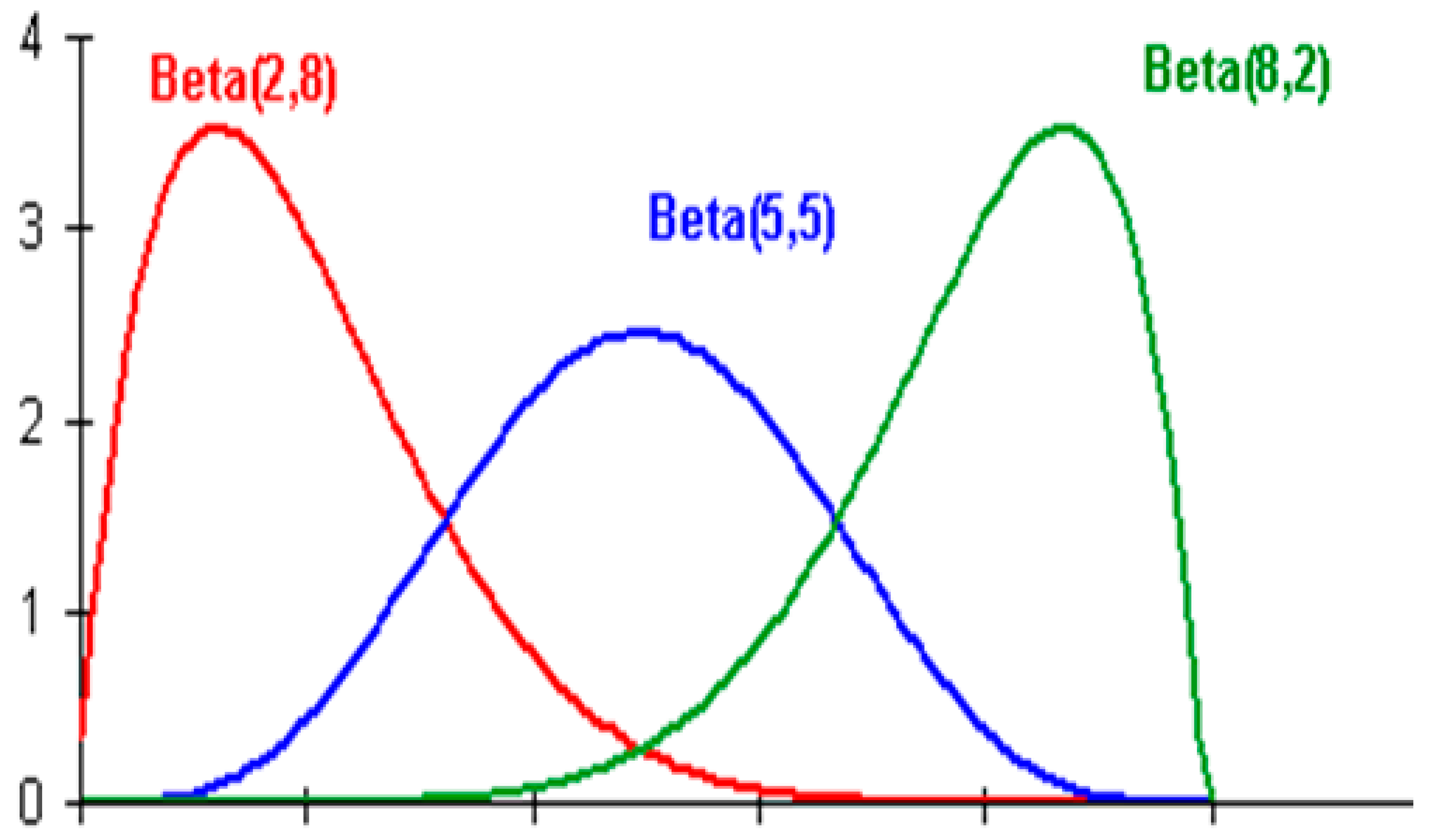
). Steijn et al. [36] have developed a method for the inclusion of uncertainty by adopting probability distributions in place of point values. This can be performed by transforming the point estimates into probability distributions. The number of parameters in the model is large, thus there is a need to focus on a narrow set of significant HOE variables. Consequently, a sensitivity analysis is conducted to determine the most influential HOE variables on the outcome. 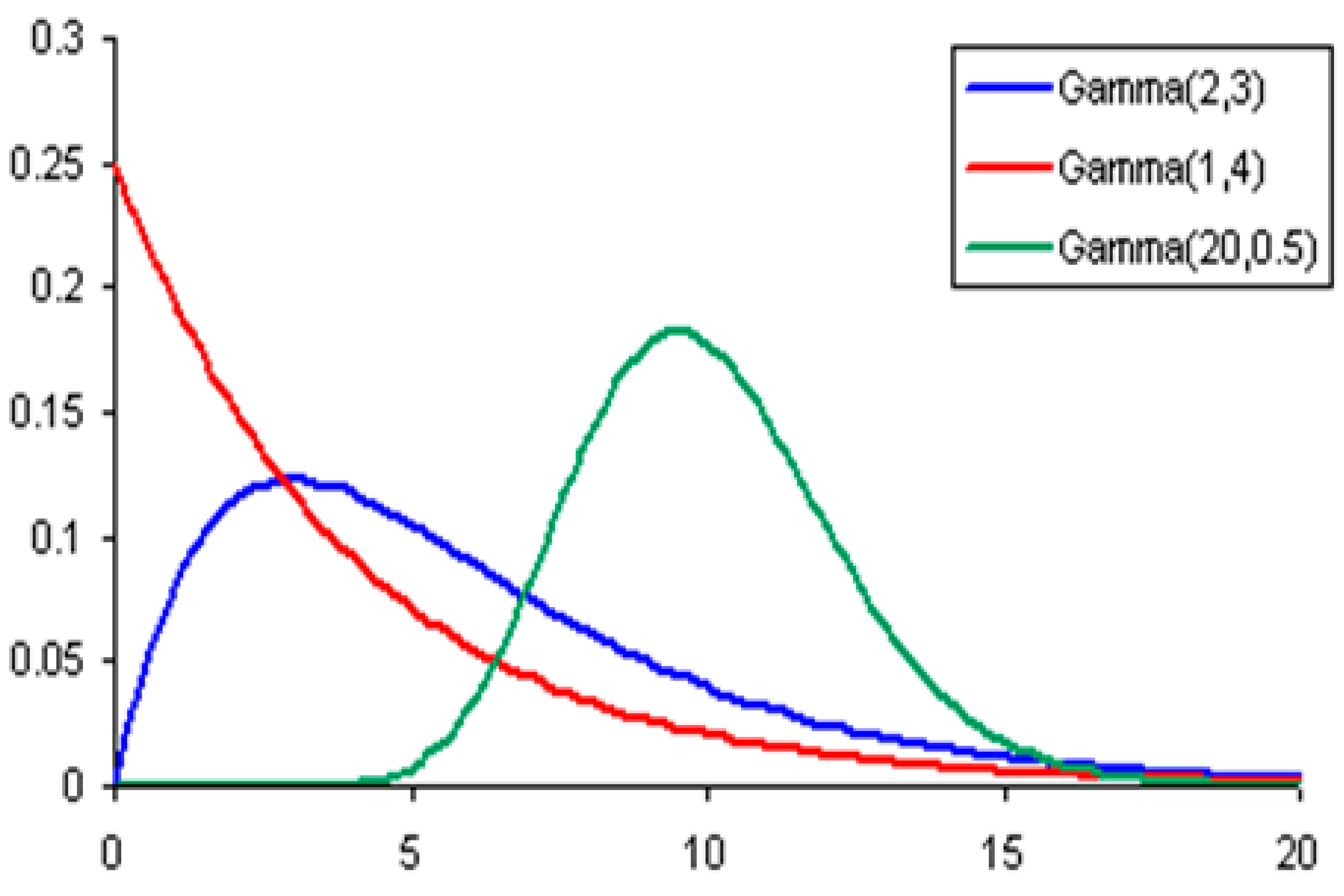To analyze the uncertainty associated with the HOE variables, the beta distribution is assumed because this distribution allows for updating with new HOE data by combining prior with posterior probability; as the number of observations increase, the distribution will become narrower as there is less uncertainty in probability of errors [36]. Beta distributions are useful to express failure probability density functions (PDFs), described by the following equation:

$$f\left(x\right)=\frac{{\left(x-p\right)}^{\left(\alpha -1\right)}{\left(q-x\right)}^{\left(\beta -1\right)}}{B\left(\alpha ,\beta \right){\left(q-p\right)}^{\left(\alpha +\beta +1\right)}}$$

(2)

where α and β indicate the number of successes and failures, respectively. The conversion from point estimation to α and β values that are required to plot a beta distribution is possible using the three-point estimation method. These three points are the lowest realistic (min), the modal (mod), and the maximum (max); the normal value for each HOE is estimated by expert judgment. PSFs are then used to determine modal, the worst-case and the best-case probability of failure through multipliers that weigh the impact of each factor. The best-case estimation was based on a scenario with realistic HOEs while in the worst-case scenario, the HOEs were assumed to have deteriorated to a point that would still realistically allow an organization to remain functional. For simplicity, the nominal modal level for each HOE-variable is considered, as represented in

Table 6. Performance shaping factors (PSFs) and range for associated multipliers.

PSF	Modal Level	Modal Multiplier	Best Case Multiplier	Worst Case Multiplier
Available time	Nominal	1	1	1
Stress and stressors	Nominal	1	1	2
Complexity	Nominal	1	1	1
Experience and training	Nominal	1	0.1	1
Procedures	Nominal	1	0.5	1
Ergonomics	Nominal	1	1	1
Fitness for duty	Nominal	1	1	1
Work processes	Nominal	1	0.8	2
Multipliers		1	0.04	4

:

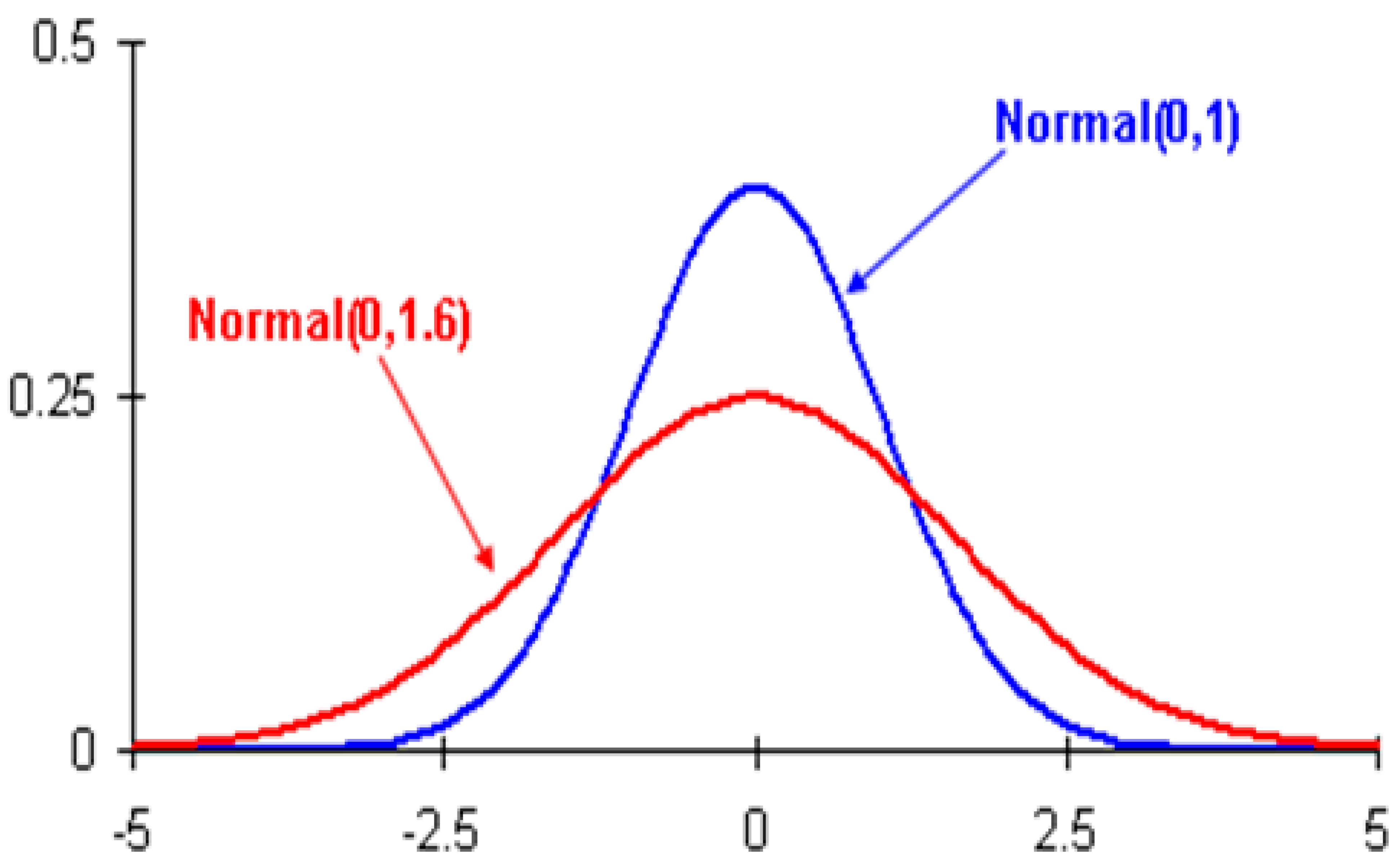
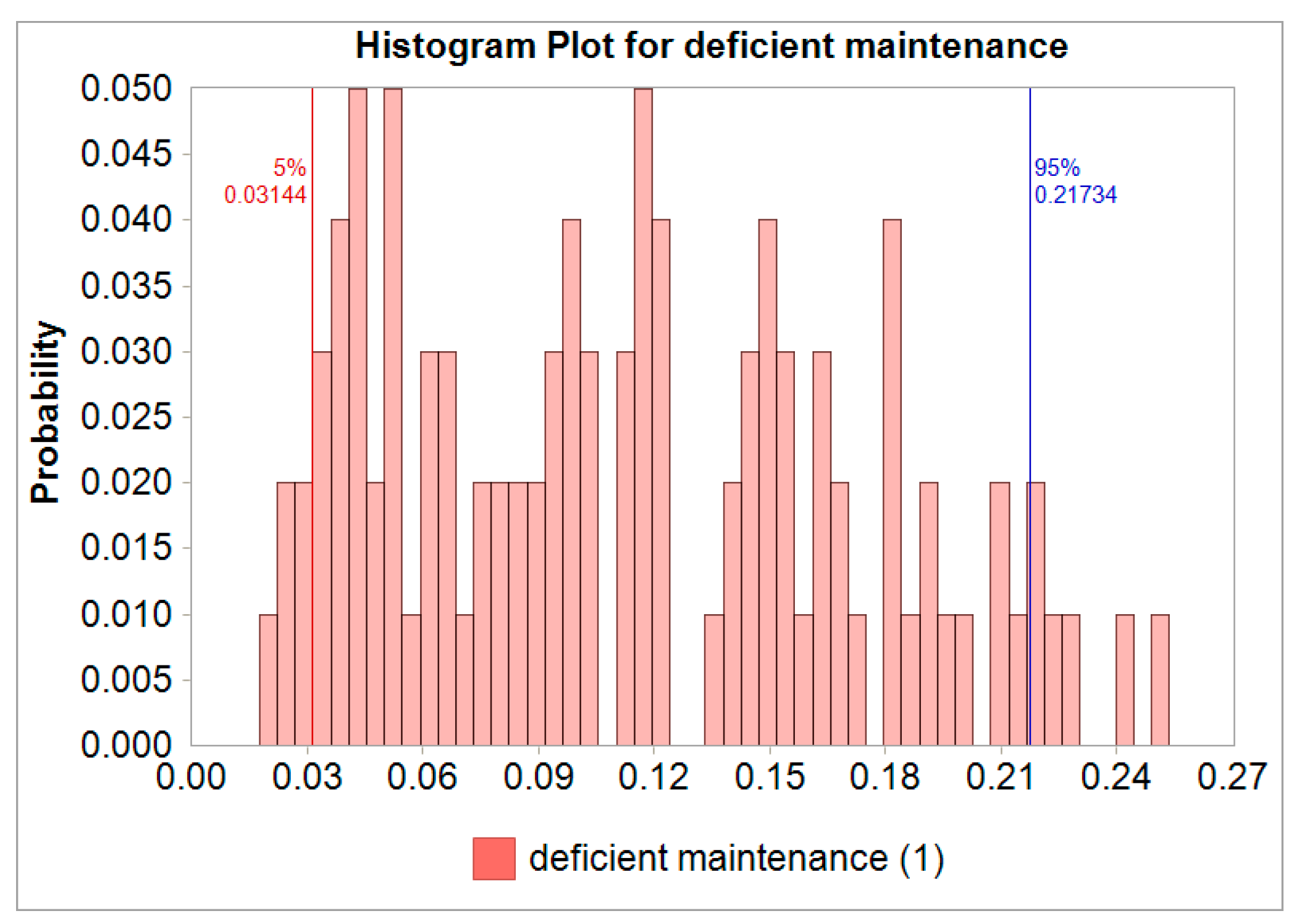
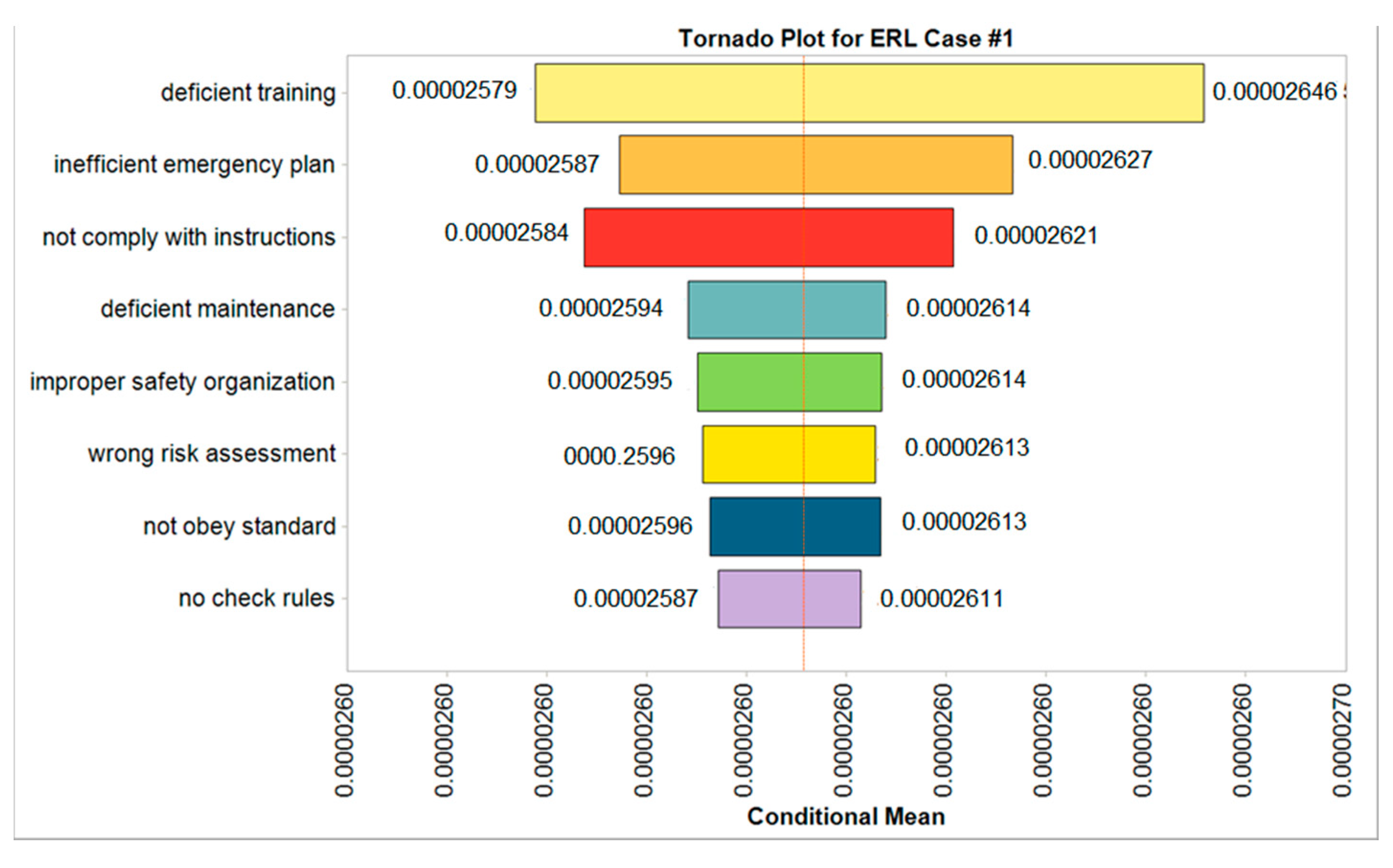
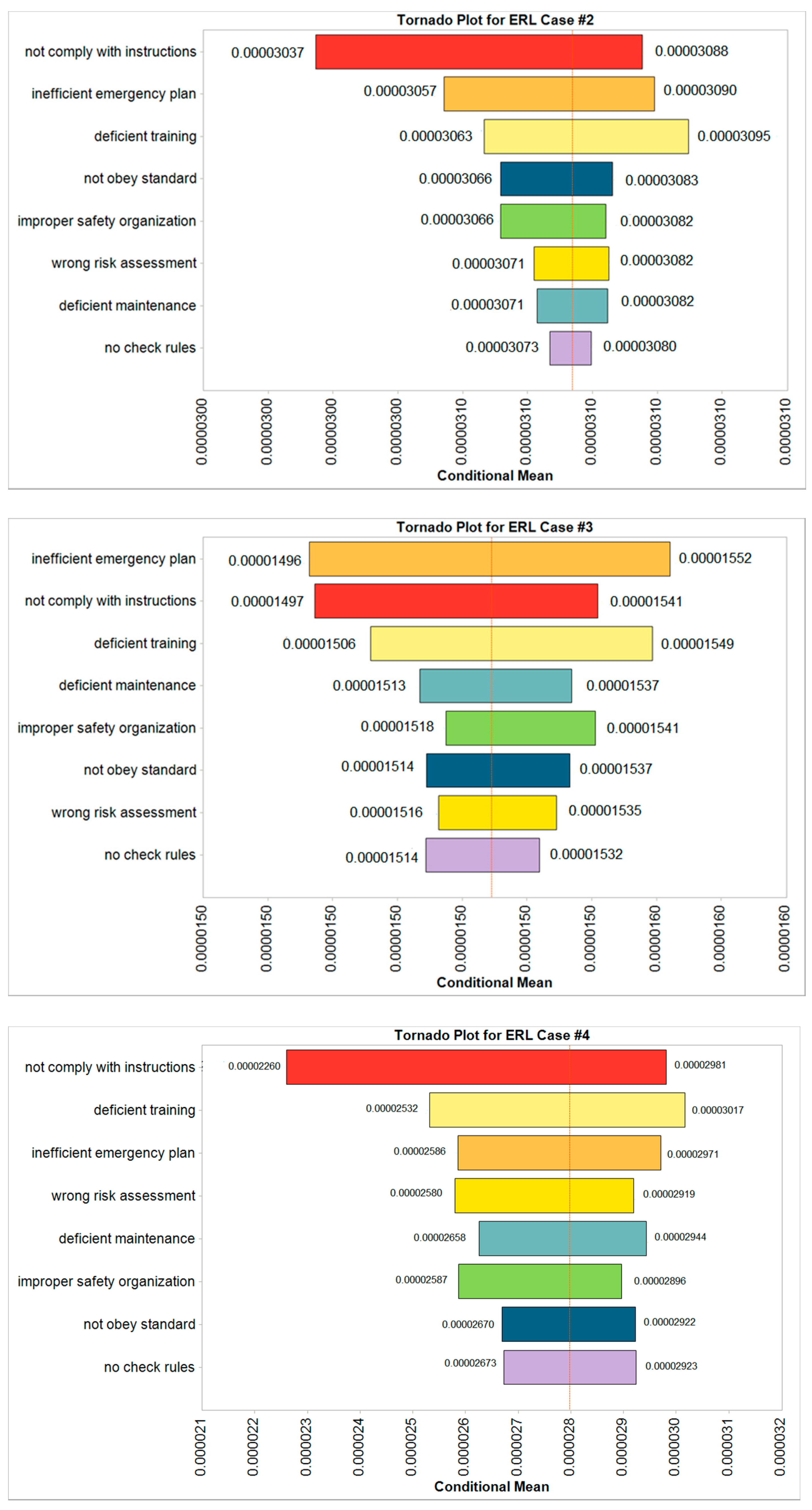
Once the probability distribution of each HOE-variable is defined, the propagation of uncertainty is calculated. A beta distribution for each of the HOE variables in the BN is assumed, such as deficient maintenance as shown in Figure 8 where y-axis represents the probability and x-axis represents the ERL values. The beta distribution for the deficient maintenance variable uses the three points as follows: minimum value = 0.0032, modal value = 0.08, maximum value = 0.32. A similar analysis is performed for the other three cases. The results of the sensitivity analyses are summarized in the Tornado Plots presented in Figure 9.

The results indicate that the most influencing HOE factors are ‘not comply with instructions’, ‘deficient training’, and ‘inefficient emergency plan’. The mean value of the ERL is highest for Case #4 when considering the HOE ‘not comply with the instruction’. The same trend is also observed for Case #4 for the other two critical HOE factors, ‘deficient training’ and ‘inefficient emergency plan’. The main HOE variables impacting the final ERL are dependent on the design type. In those scenarios/designs where there are minimal active safety measures (DTS solutions), the impact of ‘not comply with instruction’ or ‘inefficient emergency plan’ are more significant. This is clearly because when no active fire safety measures are in place, the global safety of the building relies less on the activity of an operator that would periodically check on the safety systems than on the organisational efficiency required to determine the presence of ignition sources, combustible materials or working conditions of the fire doors. The other significant HOE factors considered in the analysis are ‘no check rules’, ‘improper safety organization’, ‘wrong risk assessment’, ‘no check rules’ and ‘not obey standard’.

4.2.2. Uncertainty Analysis of HOE and ERL

The purpose of the uncertainty analysis of the ERL is to determine the HOE-related influence on risk variations in the model. While the sensitivity analysis previously conducted assesses the ranking of the contributions of the HOE inputs to the total ERL outcomes, an uncertainty analysis assesses the uncertainty in the model risk outputs that arise from the variations in HOE inputs. One of the procedural requirements in a PRA is the quantification of the uncertainties associated with the model variables. In particular, the probability values of human and organizational failures are affected by high levels of errors in estimations. There is limited literature data supporting their inclusion in a PRA, both in terms of absolute value and in terms of distribution through the probabilistic model. It is therefore of the utmost importance to estimate the distribution and range of those errors and their impact on the global level of risk.

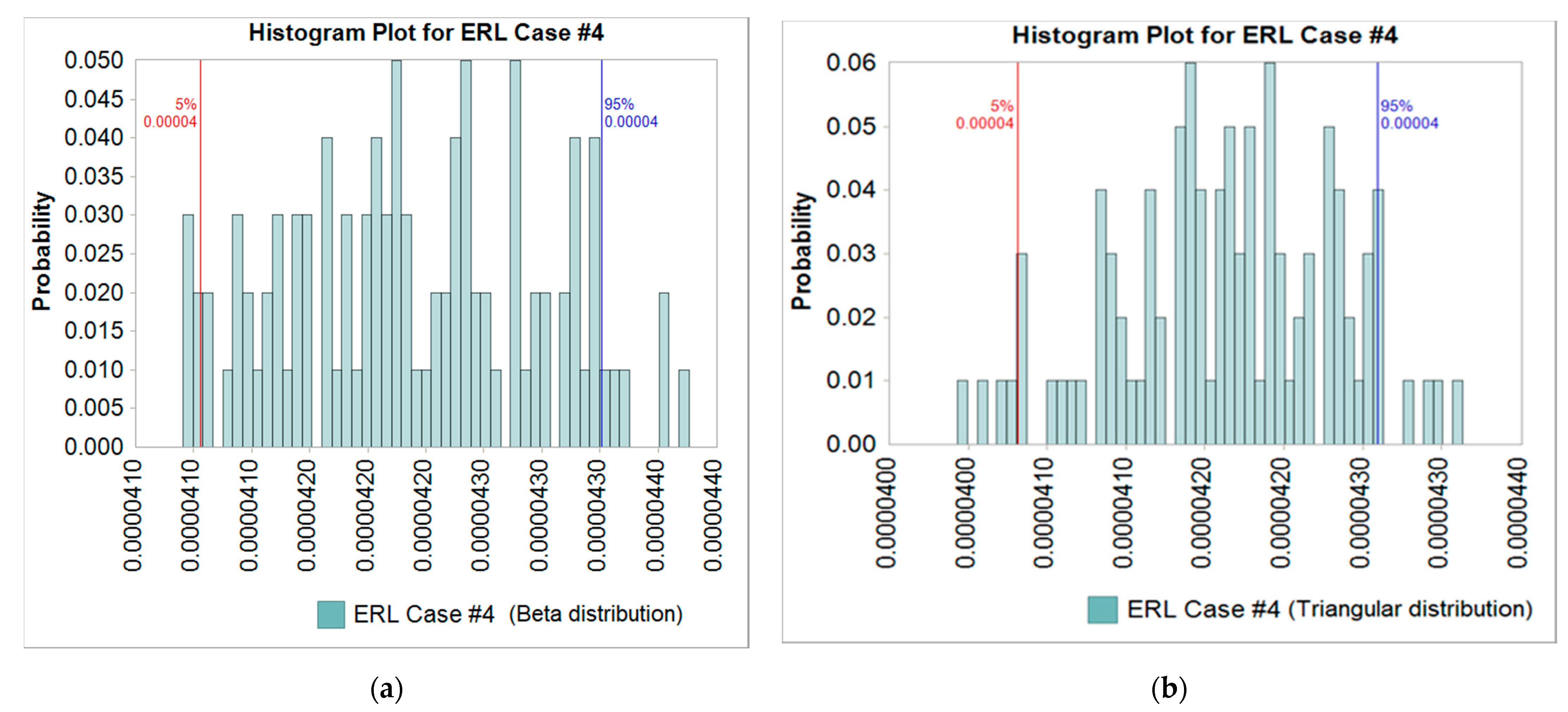
The sensitivity results show that the most influencing HOE factors are ‘not comply with instruction’, ‘deficient training’ and ‘inefficient emergency plan’. The three main variables determine important variations in the ERL of the system, up to 30% of the reference value. The minimum variations associated with the HOEs are in the order of 3–5%. The study indicates that HOEs have an important impact on the global risk level and cannot be neglected. Moreover, the more complex the system, the greater their influence. The complexity of the system is essentially due to the number of fire safety measures adopted, each of them subjected to varying maintenance regimes. The uncertainty analysis was performed based on the three most influencing HOEs identified in the sensitivity analysis in each case study. Using Case #4 as an example, when the most significant HOE factor of ‘not comply with instruction’ is simulated with 100 Monte Carlo simulations, the results are shown in Figure 10a where the y-axis represents probability values and x-axis represents the ERL values. It can be noted that the minimum probable ERL value with HOEs for Case #4 is 4.07 × 10⁻⁵ deaths/year while the maximum ERL value is 4.38 × 10⁻⁵ deaths/year. The mean value is 4.21 × 10⁻⁵ deaths/year and the standard deviation is 7.57 × 10⁻⁷. The 5% and 95% confidence interval range for uncertainty is between 4.09 × 10⁻⁵ and 4.34 × 10⁻⁵.

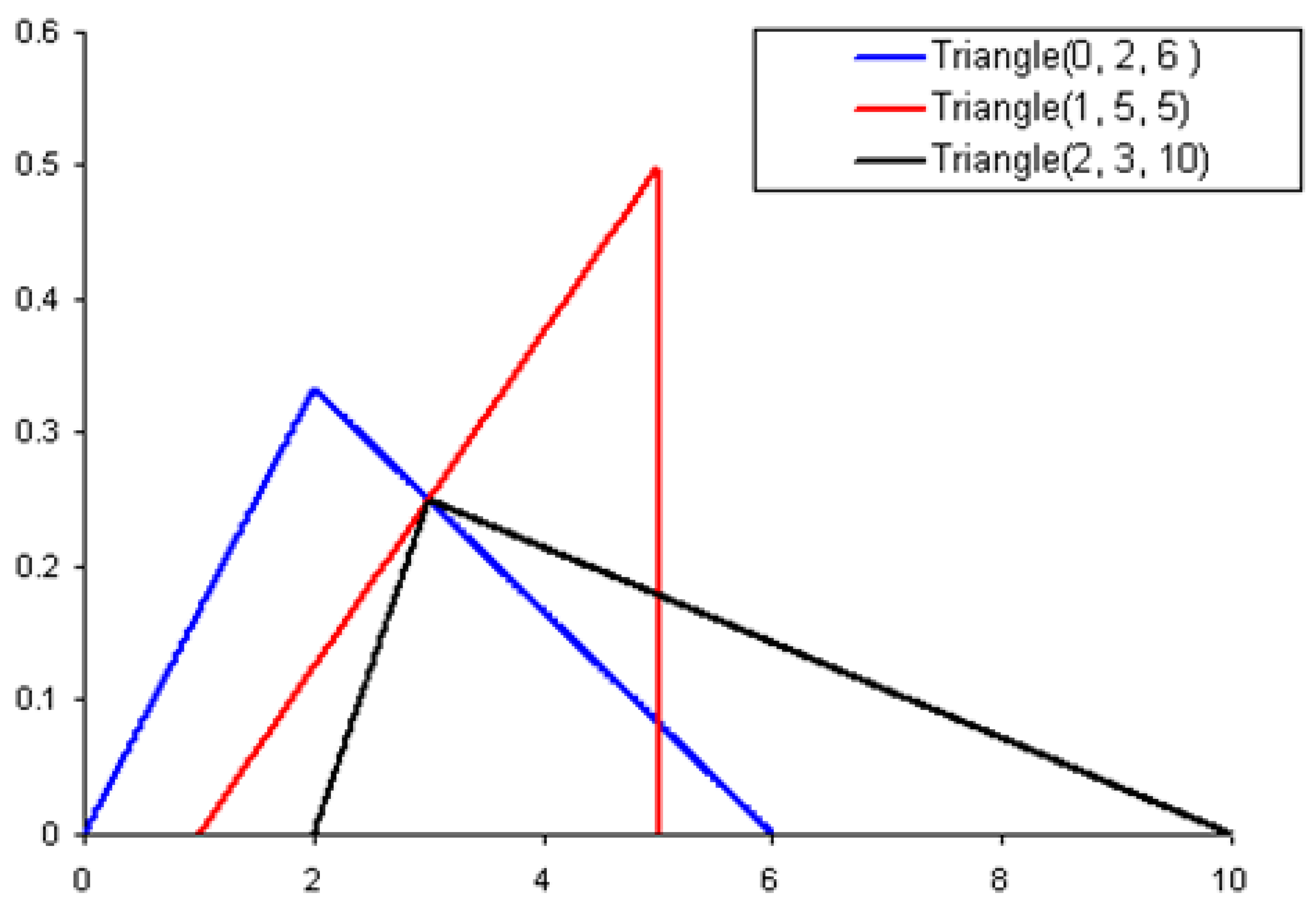
When limited information is available on the likely distributions of the key variables, the triangular distribution can be used to reflect the most likely, lowest, and highest outcomes. When using a triangular distribution for the variable ‘not comply with the instruction’, the 5% and 95% uncertainty ranges between 4.06 × 10⁻⁵ and 4.32 × 10⁻⁵ as shown in Figure 10b. This indicates that a beta or triangular distribution does not alter the uncertainty range significantly while the beta distribution produces a smoother curve.

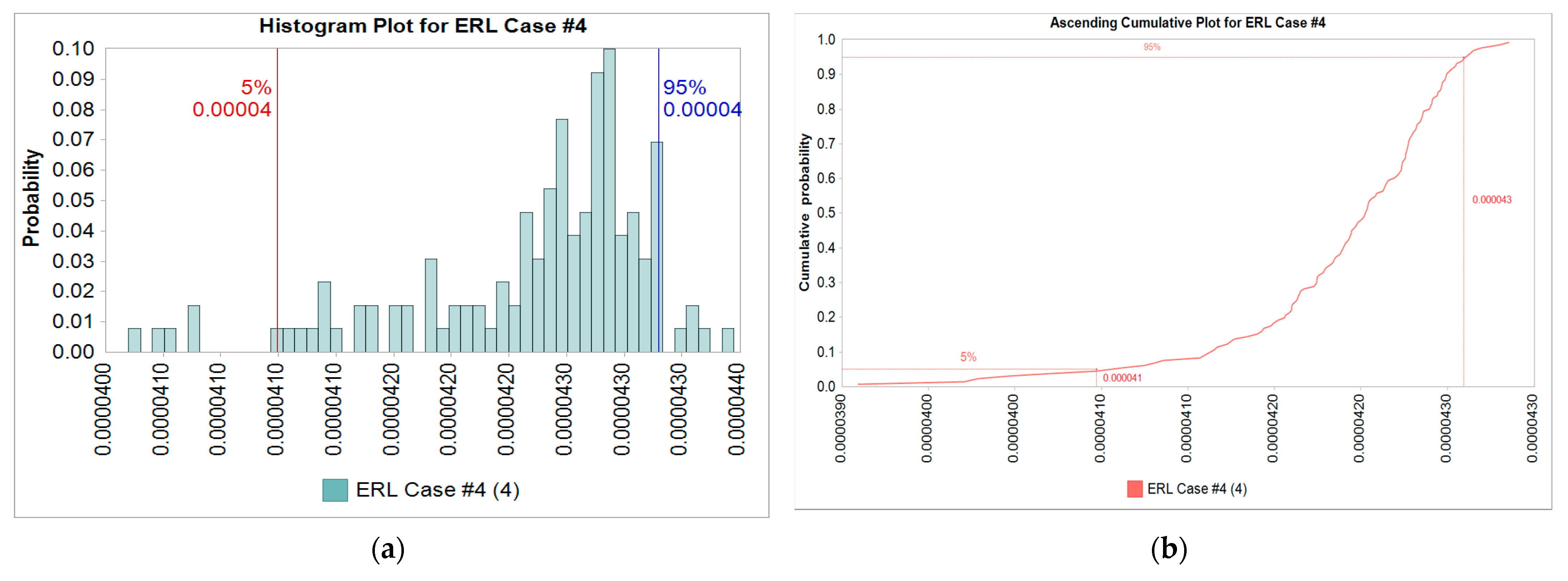
When considering the three main HOE variables and assuming a beta probability distribution, the result is shown in Figure 11a. The y-axis represents the probability and x-axis represents the ERL values. It can be noted that the outcomes of the simulations are concentrated on the right side of the histogram. The standard deviation is small at 5.40 × 10⁻⁷ with 5% and 95% uncertainty ranges from 4.15 × 10⁻⁵ to 4.30 × 10⁻⁵. The cumulative probability distribution of the single-run curve (S-curve) for Case #4 is presented in Figure 11b where the mean ERL is 4.25 × 10⁻⁵.

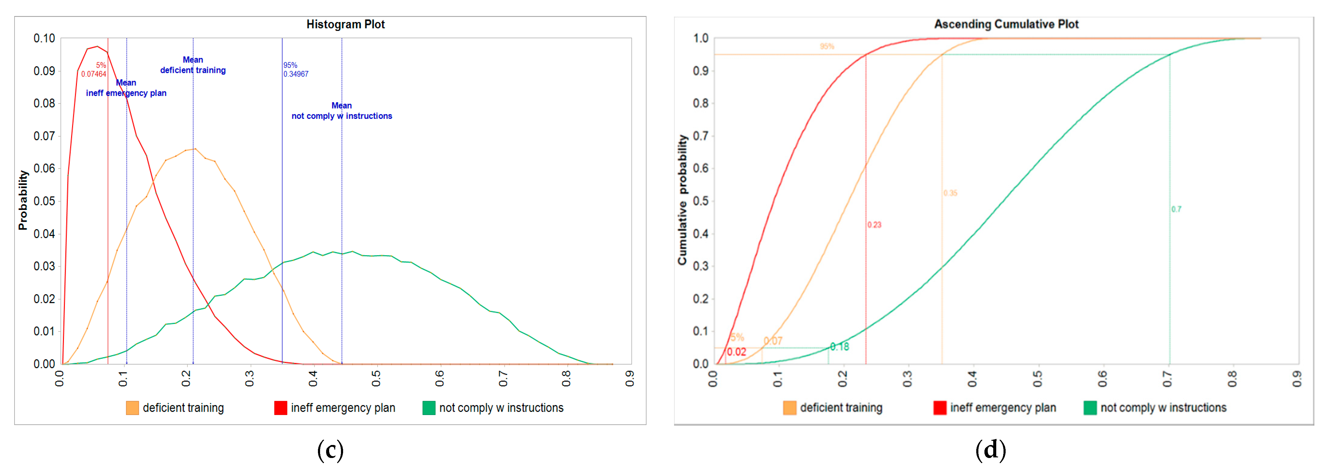
Figure 11c shows the probability density plot and Figure 11d shows the cumulative probability distribution of the three HOE input variables that have a major impact on the final ERL for Case #4. The cumulative probability plot in Figure 11d indicates that the distribution of the probability for ‘not comply with the instruction’ is centred on higher values than the other two HOE variables; its mean is 0.46 compared to 0.25 for ‘deficient training’ and 0.11 for ‘inefficient emergency plan’. Moreover, it is evident that the HOE variable ‘not comply with the instruction’ has larger variations than the other two because the difference between the 95% and the 5%-percentiles is 0.49 in absolute terms (and 1.07 relative to the mean). (Refer to Appendix C for detailed calculations).

To evaluate the uncertainty of the model due to the three variables, these values can be compared with the output of the model from the Monte Carlo simulation. In Figure 11d, the graph indicates that the difference between the 95% and the 5% value is 2.9 × 10⁻⁷. (Refer to Appendix C for detailed calculations). As expected, the HOE variable ‘not comply with instructions’ has the greatest influence on the outcome with a sensitivity of 5% followed by ‘deficient training’ at 4% and ‘inefficient emergency plan’ at 3%.

As expected, the HOE variable ‘not comply with instructions’ has the greatest influence on the outcome with a sensitivity of 5% followed by ‘deficient training at 4% and ‘inefficient emergency plan’ at 3%.

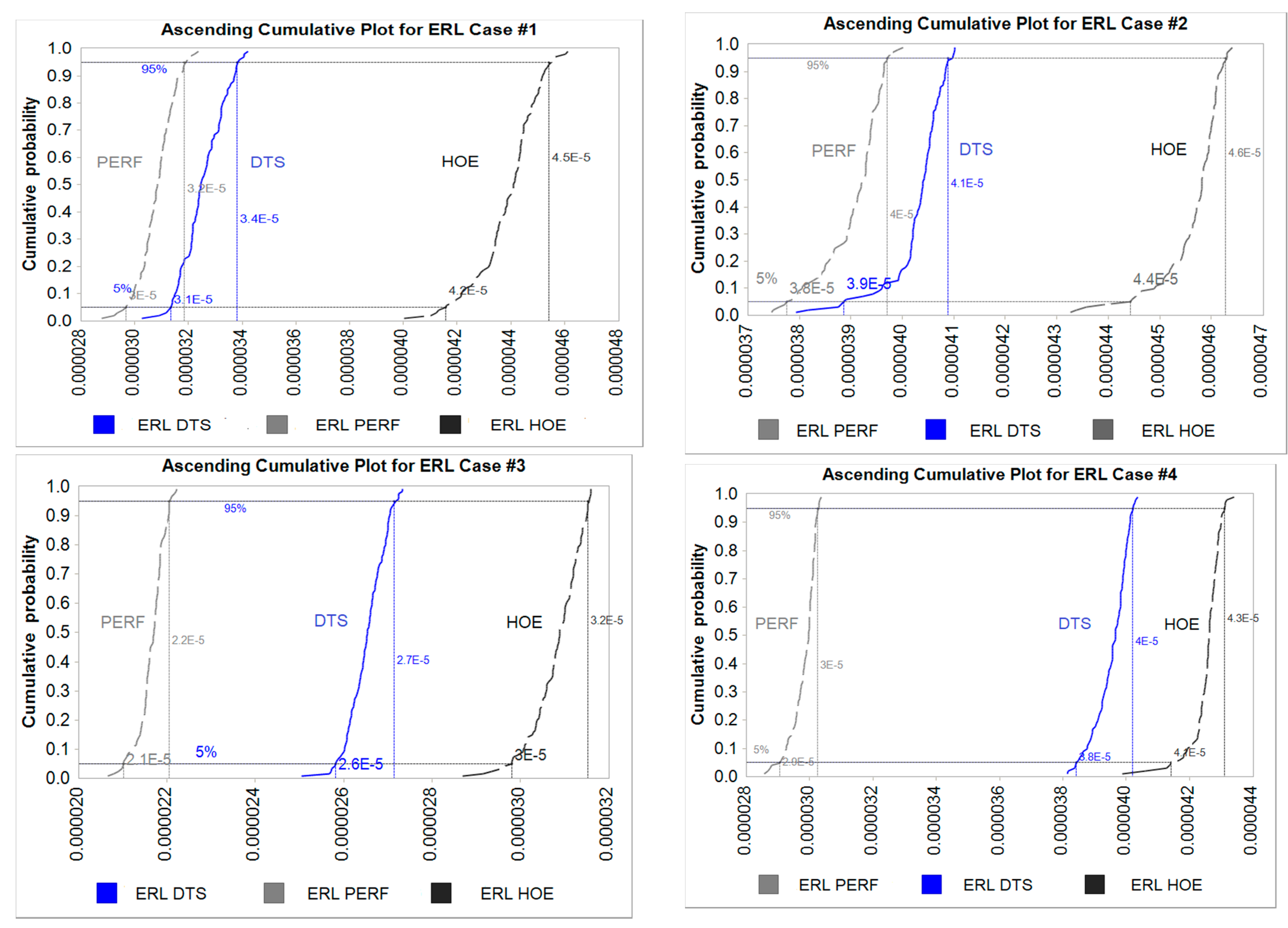
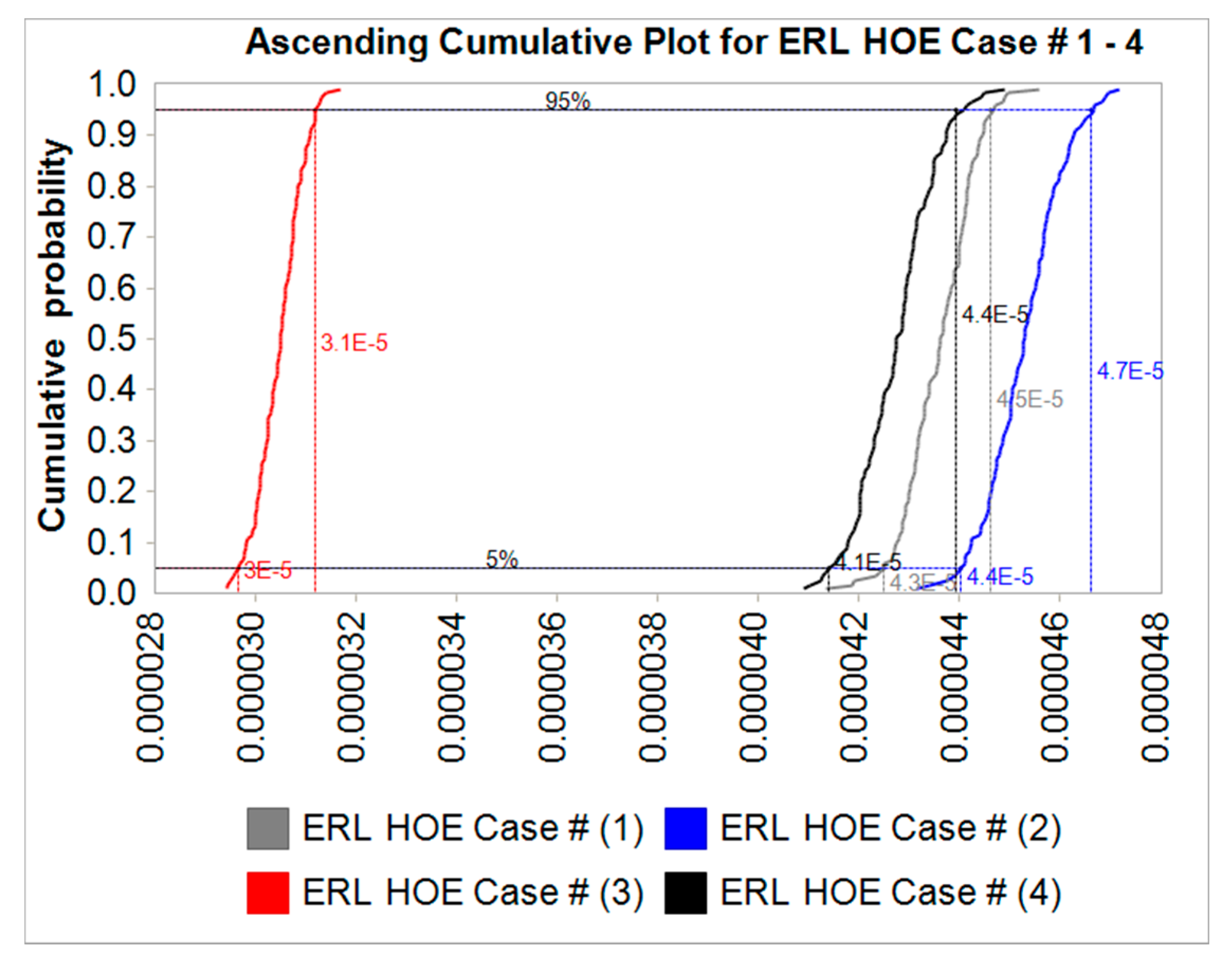
The Monte Carlo simulation runs for the ERL uncertainties for Case #1 to #4—DTS, performance and HOE solutions are plotted in the cumulative probability plots in Figure 12. It is observed that ERL for the performance solution with HOEs is higher as compared to the performance solution and DTS-based ERL values. Further, the performance solution (without HOEs) gives lower ERL as compared to the DTS solution. The results for different cases are summarized below:

• For Case#1 ERL values for the performance solution with HOEs for 5% and 95% bounds are 4.21 × 10⁻⁵ and 4.58 × 10⁻⁵, respectively. ERL values for the DTS solution for 5% and 95% bounds are 3.10 × 10⁻⁵ and 3.37 × 10⁻⁵, respectively. Similarly, ERL values for the performance solution for 5% and 95% bounds are 2.94 × 10⁻⁵ and 3.18 × 10⁻⁵, respectively. From the average value, the ERL for the performance solution with HOEs is higher by 35% compared to the DTS solution and by about 44% as compared to performance solution.
• For Case#2 ERL values for the performance solution with HOEs for 5% and 95% bounds are 4.40 × 10⁻⁵ and 4.63 × 10⁻⁵, respectively. ERL values for the DTS solution for 5% and 95% bounds are 3.91 × 10⁻⁵ and 4.10 × 10⁻⁵, respectively. Similarly, ERL values for the performance solution for 5% and 95% bounds are 3.78 × 10⁻⁵ and 3.97 × 10⁻⁵, respectively. From the average value, the ERL for the performance solution with HOEs is higher by 13% as compared to the DTS solution and by about 16% as compared to performance solution.
• For Case#3 ERL values for the performance solution with HOEs for 5% and 95% bounds are 3.01 × 10⁻⁵ and 3.15 × 10⁻⁵, respectively. ERL values for the DTS solution for 5% and 95% bounds are 2.58 × 10⁻⁵ and 2.72 × 10⁻⁵, respectively. Similarly, ERL values for the performance solution for 5% and 95% bounds are 2.10 × 10⁻⁵ and 2.22 × 10⁻⁵, respectively. From the average value, the ERL for the performance solution with HOEs is higher by 16% as compared to the DTS solution and by about 41% as compared to performance solution.
• For Case#4 ERL values for the performance solution with HOEs for 5% and 95% bounds are 4.15 × 10⁻⁵ and 4.30 × 10⁻⁵, respectively. ERL values for the DTS solution for 5% and 95% bounds are 3.83 × 10⁻⁵ and 4.02 × 10⁻⁵, respectively. Similarly, ERL values for the performance solution for 5% and 95% bounds are 2.92 × 10⁻⁵ and 3.03 × 10⁻⁵, respectively. From the average value, the ERL for the performance solution with HOEs is higher by 7% as compared to the DTS solution and by about 42% as compared to the performance solution.

The results also indicate that uncertainties associated with the ERL point estimates are small. At the same time, the low standard deviations as shown in

Table 7. Uncertainty analysis of ERL for Case #1 to #4.

Design	Sampling	Case #1	Case #2	Case #3	Case #4
DTS	Mean	3.25 × 10−5	4.02 × 10−5	2.66 × 10−5	3.97 × 10−5
	5%CI	3.10 × 10−5	3.91 × 10−5	2.58 × 10−5	3.83 × 10−5
	95%CI	3.37 × 10−5	4.11 × 10−5	2.72 × 10−5	4.02 × 10−5
	Standard deviation	7.66 × 10−7	5.87 × 10−7	4.37 × 10−7	5.43 × 10−7
Performance	Mean	3.05 × 10−5	3.89 × 10−5	2.17 × 10−5	2.98 × 10−5
	5%CI	2.94 × 10−5	3.78 × 10−5	2.10 × 10−5	2.92 × 10−5
	95%CI	3.18 × 10−5	3.97 × 10−5	2.22 × 10−5	3.03 × 10−5
	Standard deviation	7.78 × 10−7	5.27 × 10−7	3.56 × 10−7	3.79 × 10−7
HOE	Mean	4.39 × 10−5	4.56 × 10−5	3.09 × 10−5	4.25 × 10−5
	5%CI	4.21 × 10−5	4.40 × 10−5	3.01 × 10−5	4.15 × 10−5
	95%CI	4.58 × 10−5	4.63 × 10−5	3.15 × 10−5	4.30 × 10−5
	Standard deviation	1.14 × 10−6	6.90 × 10−7	4.18 × 10−7	5.40 × 10−7

signifies that the data points are closely distributed around the mean values.

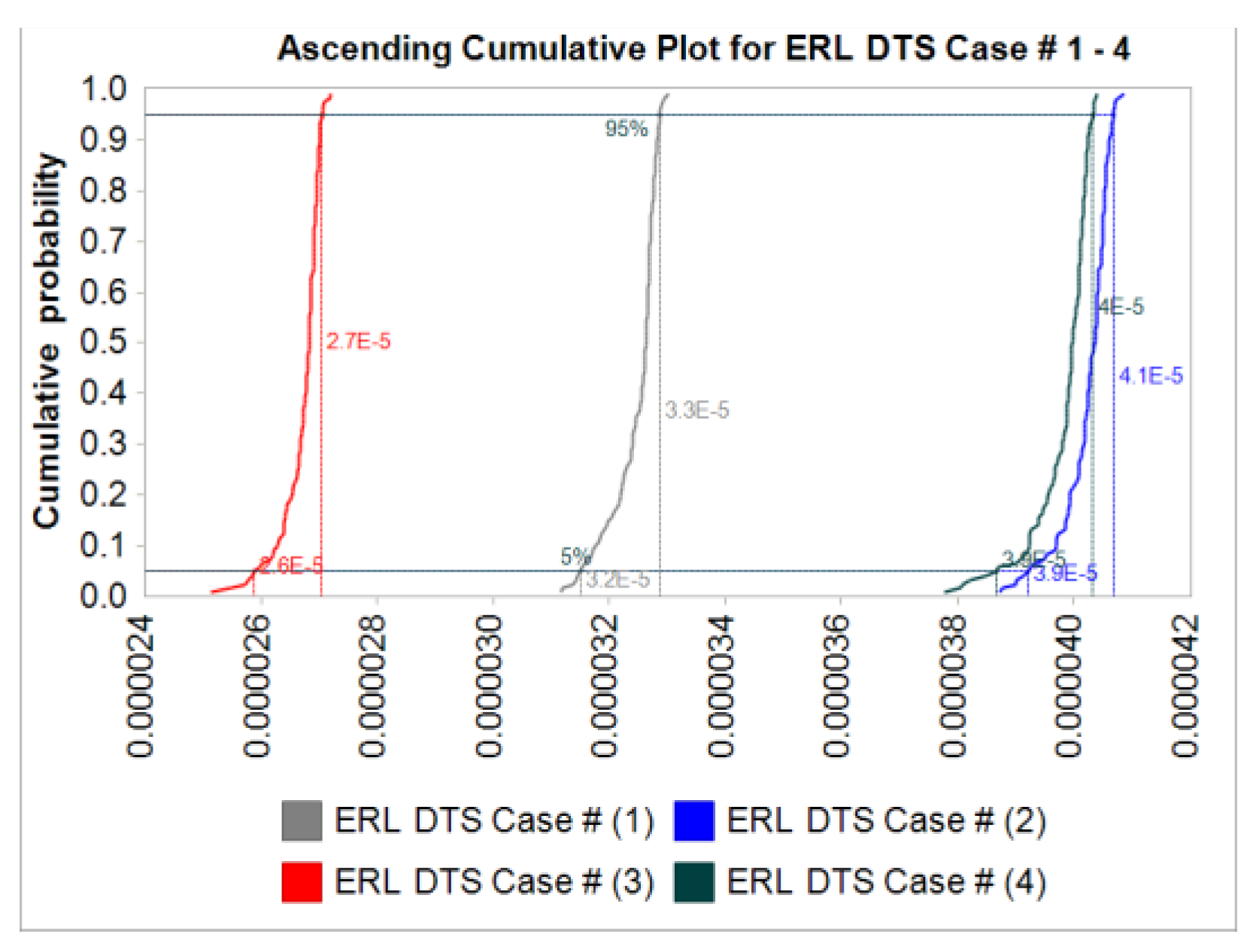
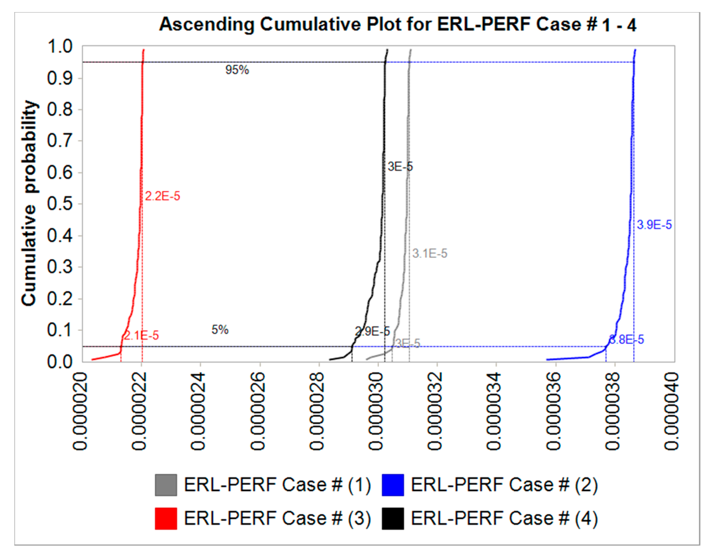
Figure 13, Figure 14 and Figure 15 show the ERL cumulative distribution plots for the DTS, performance and performance solution with HOEs to facilitate a direct comparison of the ERL for the case studies. The ERL uncertainty values are summarized in Table 7. Here again, ERL values are compared for DTS and performance solutions along with HOEs for four cases. The ERL is highest for the performance solution with HOEs followed by the DTS solution and then the performance solution. The ERL value is highest for Case #4 which has the largest floor area.

Detailed results are summarized below:

• For the DTS solution, the ERL value is highest for Case #2 followed by Case #4, #1 and #3 in descending order.
• For the performance solutions, the ERL value is highest for Case #2 followed by Case #1, #4 and #3 in descending order.
• When HOEs are considered, the ERL value is highest for Case #2 followed by Case #1, #4 and #3 in descending order.
• The average across different cases shows that the performance solution gives the lowest ERL with an average value of 3.02 × 10⁻⁵ whereas for DTS solution it is 3.48 × 10⁻⁵.

When HOEs are considered in the analysis, the ERL increases to 4.07 × 10⁻⁵, considering it is average value across different cases. Thus, across different cases, HOEs can increase the ERL value by as much as 42% compared to the performance solution. Further, the performance solution gives a lower value of ERL by much as 33% as compared to DTS solution.

4.3. Societal Risk Assessment and Uncertainty Analysis

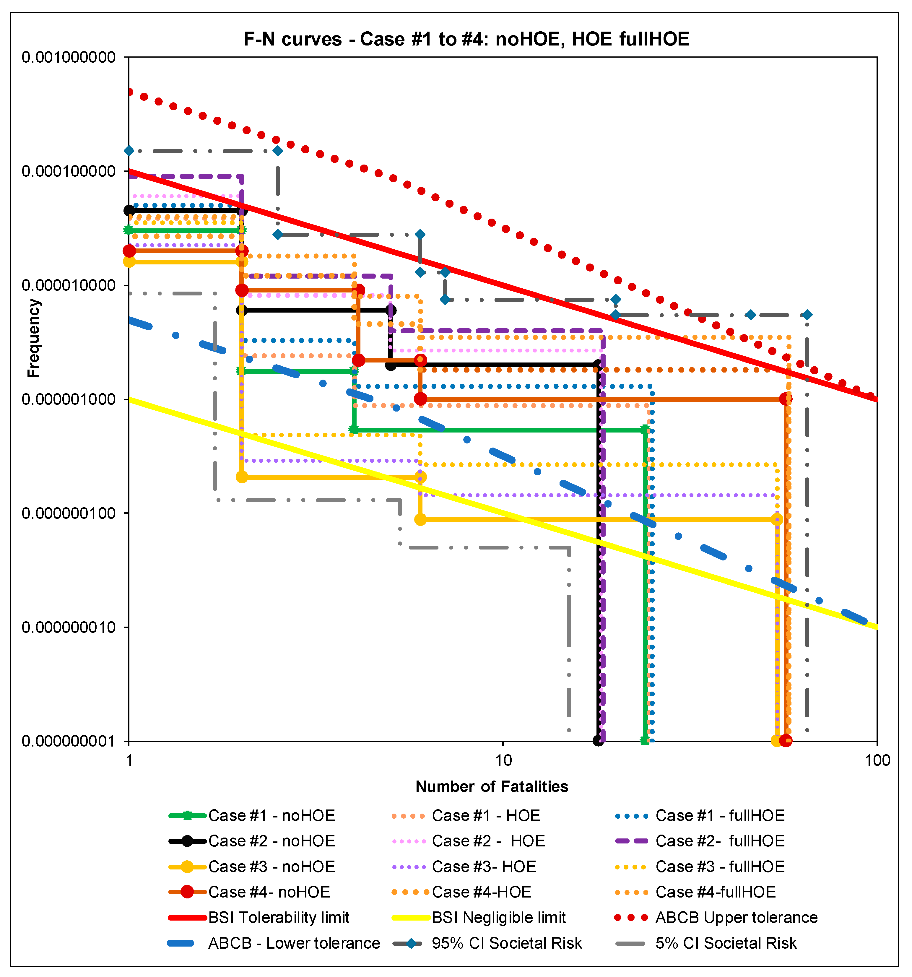
To assess the risk tolerability of various design solutions, F-N curves are constructed to enable comparison of SR for each case study. Figure 16 shows the F-N curves with and without HOEs for Case #1 to #4. ABCB tolerability curves are represented graphically by red dotted and blue dot-dash diagonal lines and are similar to British Standards Institution Published Documents (BSI) PD−7974−7:2019 [37] tolerability limits which are represented by red and yellow diagonal lines. However, the rate of change in allowable frequency is much faster (steeper slope) than BSI. The ABCB slope of −1.5 indicates a higher risk aversion than BSI’s neutral risk aversion slope of −1 [37]. The area between the tolerability curves defines the region where a design is considered to be safe, or as low as reasonably practicable (ALARP). The upper and lower bound uncertainties in SR are presented as 95% and 5% Confidence Intervals are represented by black dash-dot and grey dash-dot lines, respectively. The uncertainty analysis generates an area plot for a certain level of confidence in the F-N curve with upper (95%) and lower (5%) bounds of Societal Risk instead of only one mean F-N curve. The methodology to generate these uncertainty bounds is based on Sun et al. [38] described in Appendix D.

To assess the risk tolerability of various design solutions, F-N curves are constructed to enable comparison of SR for each case study. Figure 16 shows the F-N curves with and without HOEs for Case #1 to #4. ABCB tolerability curves are represented graphically by red dotted and blue dot dash diagonal lines and are similar to British Standards Institution Published Documents BSI PD−7974−7:2019 [37] tolerability limits which are represented by red and yellow diagonal lines. However, the rate of change in allowable frequency is much faster (steeper slope) than BSI. The ABCB slope of −1.5 indicates a higher risk aversion than BSI’s neutral risk aversion slope of -1 [37]. The area between the tolerability curves defines the region where a design is considered to be safe, or as low as reasonably practicable (ALARP). The upper and lower bound uncertainties in SR are presented as 95% and 5% Confidence Intervals are represented by black dash-dot and grey dash-dot lines, respectively. The uncertainty analysis generates an area plot for a certain level of confidence in the F-N curve with upper (95%) and lower (5%) bounds of Societal Risk instead of only one mean F-N curve. The methodology to generate these uncertainty bounds is based on Sun et al. [38] described in Appendix D.

The inclusion of HOEs in the analysis results in variations to SR values as shown in the F-N plots in Figure 17 for Case #1 to #4. The following observations can be made from Figure 16. For all cases where HOEs are considered, SRs are higher than the corresponding case with no HOEs. All cases are below the upper tolerability bounds indicating acceptable SRs, however, when HOEs are considered, Case #2 marginally exceeds BSI tolerance but meets ABCB acceptable limits. Case #4 exceeds both BSI and ABCB tolerability limits. When confidence-interval uncertainty bounds are considered, Case #2 marginally meets ABCB upper tolerability limits while Case #4 clearly exceeds the tolerability limits. To lower the curve such that it falls in the ALARP region, either additional fire safety measures can be installed, or systems reliability can be improved. Among the four cases, Case #4 results in maximum SR. This is followed by Case #2, Case #1 and Case #3 in decreasing order. For case #3 and #4, the F-N curves are shifted to the right resulting in higher consequences even though frequencies are within similar range as the other two cases. The CI-95% uncertainty bounds indicate that Case #2 & #4 exceed the BSI upper tolerance limit but only Case #4 exceeds the ABCB upper tolerance limit. Thus, when uncertainty ranges are considered, tolerability thresholds can be exceeded in some cases (Case #2 & #4) when mean values do not.

4.4. System Dynamics Risk Modelling, Sensitivity and Uncertainty Analysis

The assessment of risk in the SD model allows for an integrated analysis of HOE factors and their nonlinear interactions and feedback loops. The SD model also accounts for the delays and more realistic analysis of risk variation over time. When maintenance of a safety system is not performed for prolonged periods, risk will trend upwards over time and there can be a duration in which risk exceeds a critical or safe value. The SD model identifies the point in which the maintenance regime of safety systems needs to be conducted. System dynamics describe the level of uncertainty of diverse situations. This technique is specifically useful when variables are interlinked, and data is indistinct. In this model, some variables vary with time and simultaneously interact with other variables. Thus, the state of a variable is both time dependent and state dependent with respect to other variables. The time slice in a SD model is a snapshot of the BN at different instances of time (Figure 17).

The conditional probability table (CPT) is the transition matrix that represents the time slice and provides insights into the transformation of the different nodes across the model and describe the causal relationships within the nodes. The mathematical model describing the state and time dependency is given by:

$$P\left(X,Y\right)={\displaystyle \prod }_{t=0}^{T}P\left(x_t|x_{t-1}\right){\displaystyle \prod }_{t=0}^{T}P\left(y_t|x_t\right)P\left(x_0\right)$$

(3)

where:

• X, $x_t, x_{t-1}$ are state variables; Y, $y_t, y_{t-1}$ are observable variables;
• $P\left(x_t|x_{t-1}\right)$ gives time dependencies between states;
• $P\left(y_t|x_t\right)$ gives state dependencies between the variables;
• $P\left(x_0\right)$ is initial state distribution.

In the SD model, the flow variables are time-varying terms. For example, the rate of change (RoC) of the number of checks (NoC)) for perceived safety (ps) is given by:

$$RoC\left(t\right)=5 \frac{d}{dt}\left(ps\right)$$

(4)

On the other hand, stock variables, refer to the integrated value of the flow variables. Thus, a stock variable refers to the accumulated value of the flow variable in a given time frame. For the above example, a stock variable NoC is given by:

$$NoC=12+ \int RoC\left(t\right)dt$$

(5)

In the present analysis, random perturbations on input parameters are performed and risk is computed at each of the time instants. The nodes of the SD are mapped from the corresponding nodes in the BN model. The mapped SD model is represented in Figure A5 in Appendix A. A sample schematic showing reliability change due to time and state change is shown in Figure 18. The SD model, thus, brings out the effects of deficient training and inefficient emergency plan from the analysis.

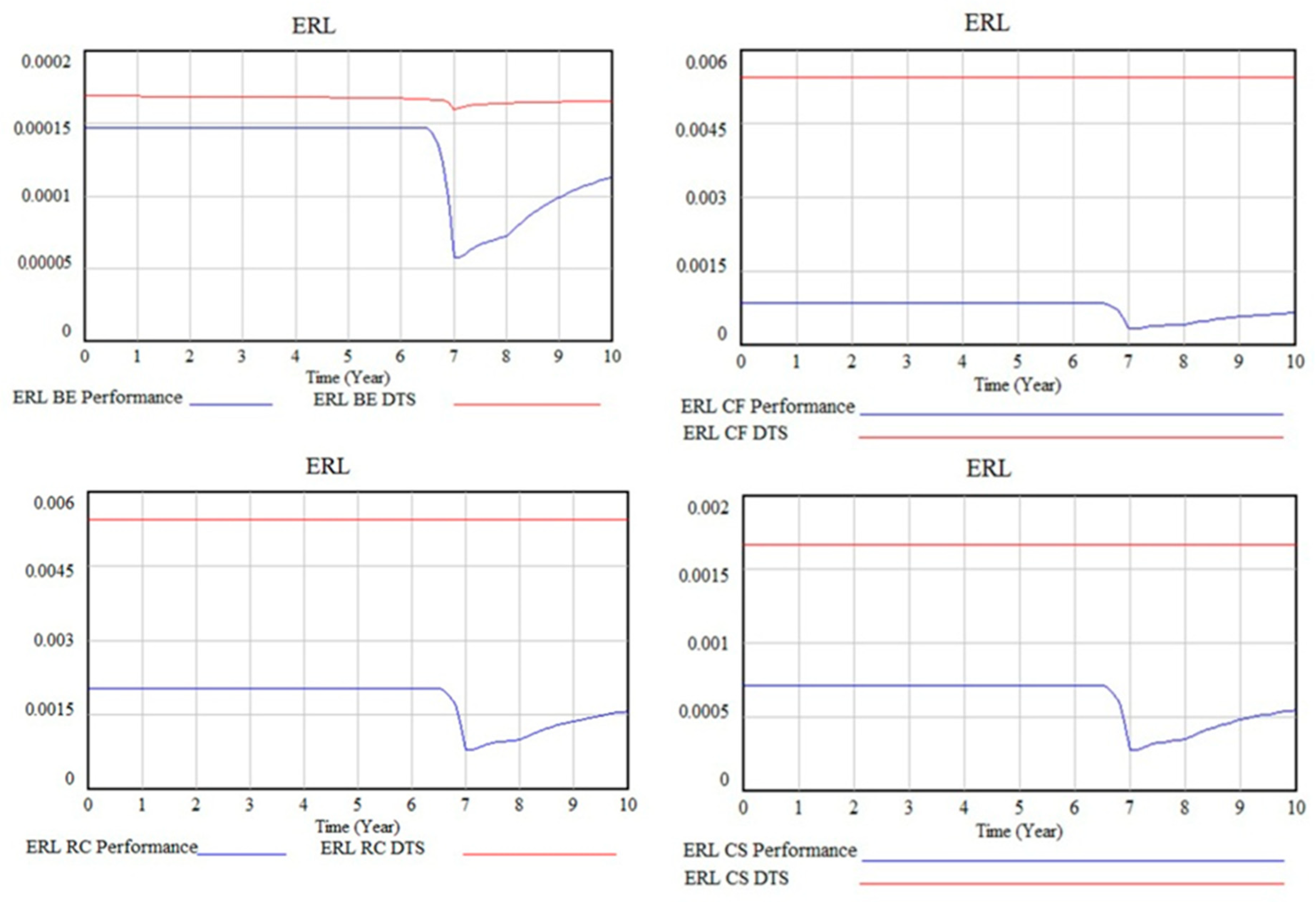
The results from the SD simulation are reported in Figure 19 which compare the DTS to the performance solutions for each design scenario for Case #1 (ABCB).

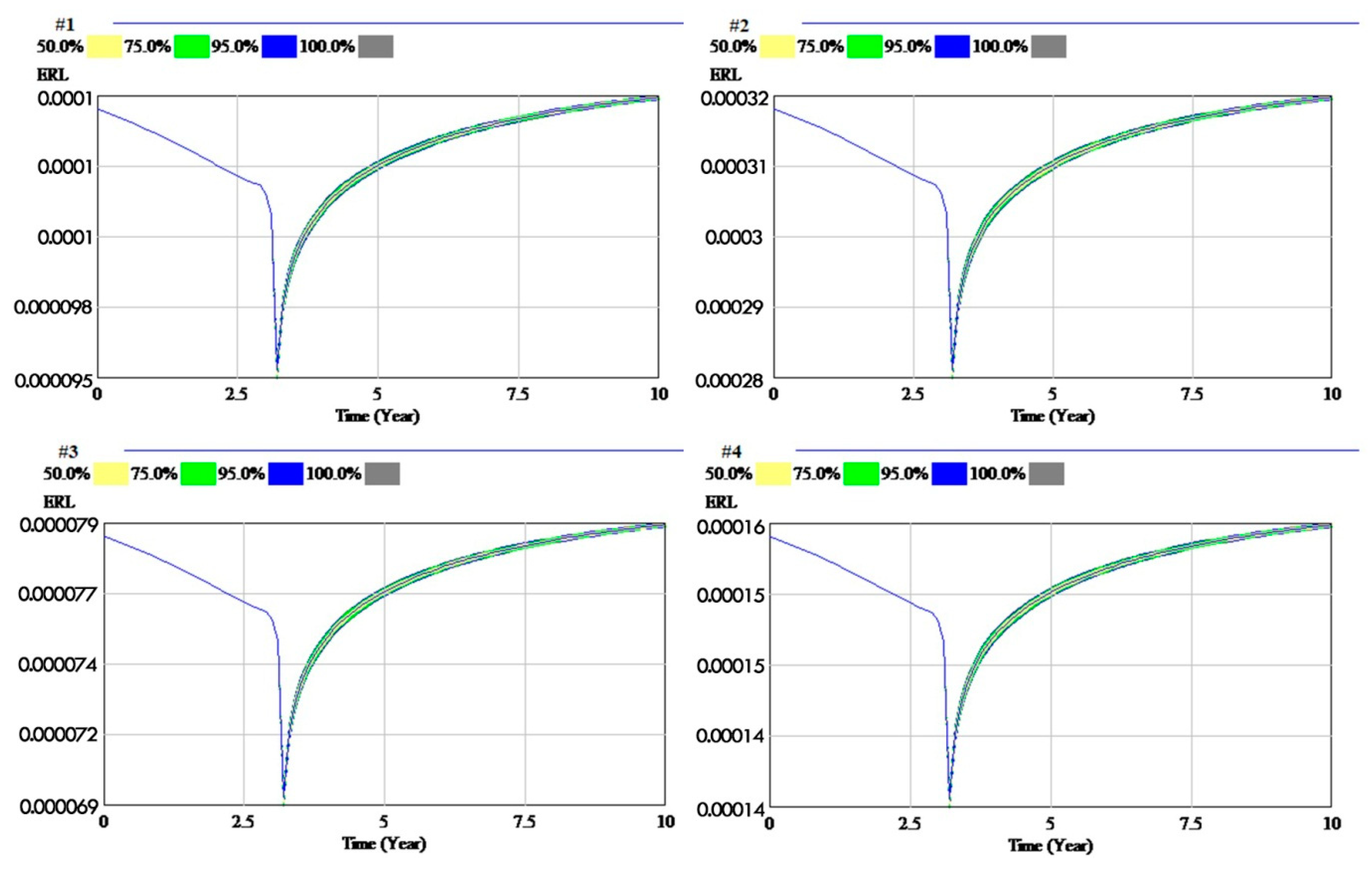
During the 10-year life span considered, the performance solution shows a lower level of risk than the DTS solution. It can also be noted that there is no variation in risk for the DTS solution over 10 years; this is because the DTS solution has no active fire protection measures (detection or suppression system), hence no HOEs can significantly alter the level of risk. However, outside the active protection system, it is always possible that HOEs reduce the reliability of passive protection systems (for example, obstructions of the exits and refurbishment activities) but they are not modelled in the T-H-O-Risk model. In the risk-over-time curve related to the performance solutions, the level of risk reduces after a seven year-long period of stability, because the building maintenance team has developed a thorough knowledge of the reliability of safety systems. At the same time, the perception of risk is reduced because little or no accidents have occurred during the initial lull period and a lax attitude towards maintenance procedures takes over. Consequently, the operator reliability falls and reduces the effectiveness of the sprinkler system. When the building management realises that the level of organization is not as effective as planned, countermeasures are activated, which in turn improves risk indicators although uncertainty is highest around year seven. Risk again increases with time in the final years of the 10-year period due to the relaxation of measures, as expected.

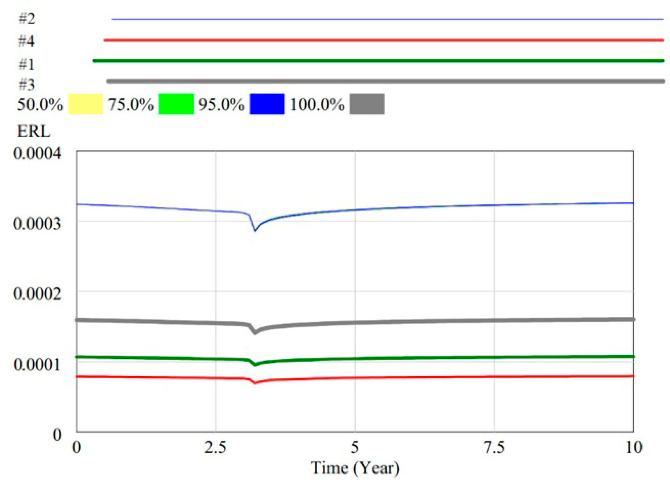
All the curves exhibit similar behaviour, experiencing a reduction in risk level after seven years and a subsequent increase due to relaxation of the rules (Figure 20). It can be noted that the different curves shift vertically according to the various global risk value as shown in Figure 21.

It is observed that the sensitivity of the curves to the HOE parameter results in no variations in the scale of the dynamic curve, so the rankings of the four designs are not affected by that parameter.

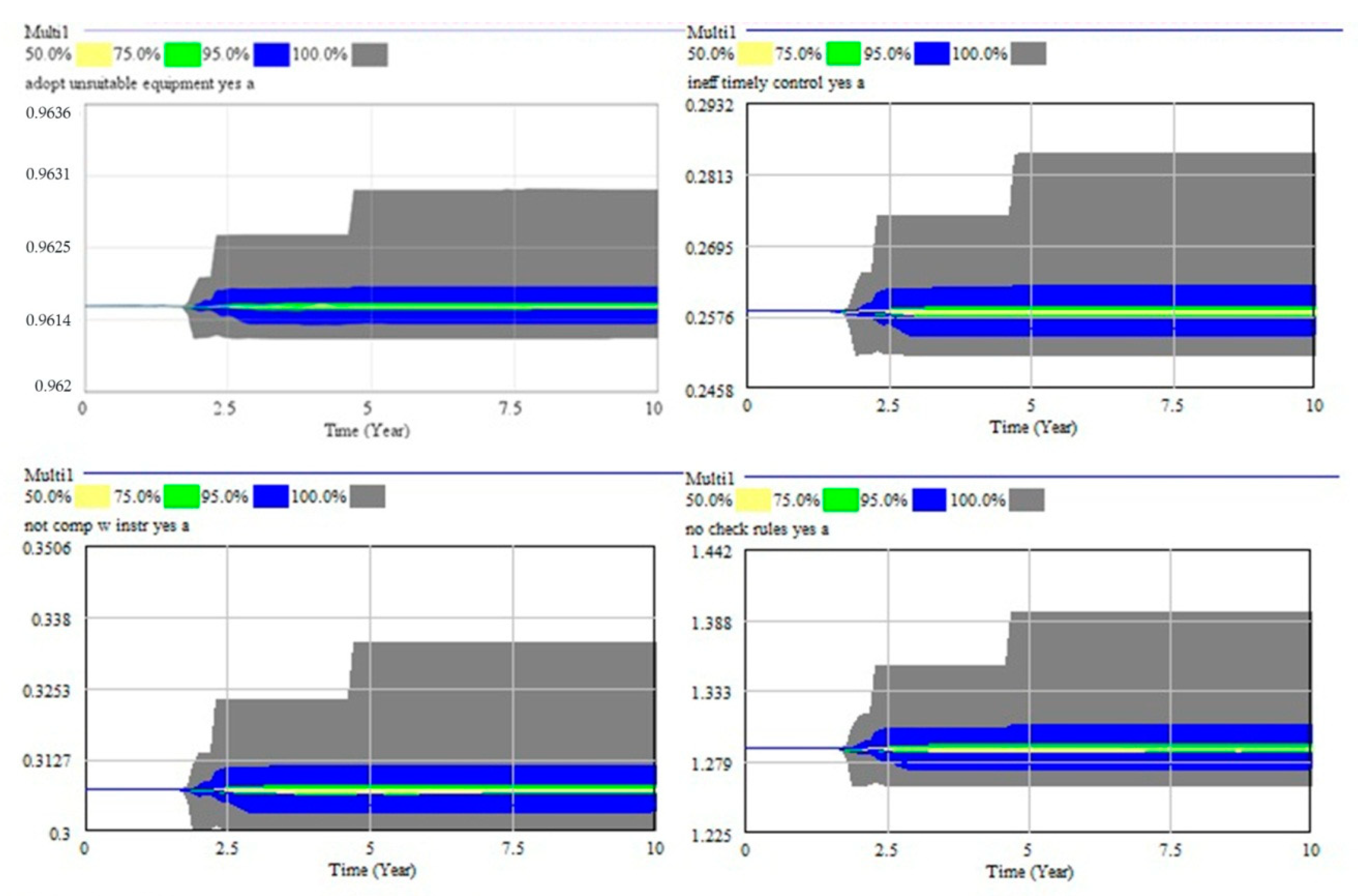
Sensitivity analysis was further conducted on key variables in the SD model to assess model robustness and to explore how uncertainty influences the analysis of different safety systems and reliability of model outputs. The first step is an investigation of the parameters with the most influence on the HOE variables (target). Most of the model parameters have little influence on the outcome, so that they do not produce noticeable variations in the target variable. The impact of a parameter can be assessed in relationship to every target variable; only if the sensitivity is above a determined value (25%) would the parameter need further analysis. For each HOE variable there are parent nodes that have low influence, such as ‘Probability of valve closed’, which has a sensitivity of 0.1% related to the target value ‘adopt unsuitable equipment’. There is negligible impact of an open valve on the final result, as it provides very small variations.

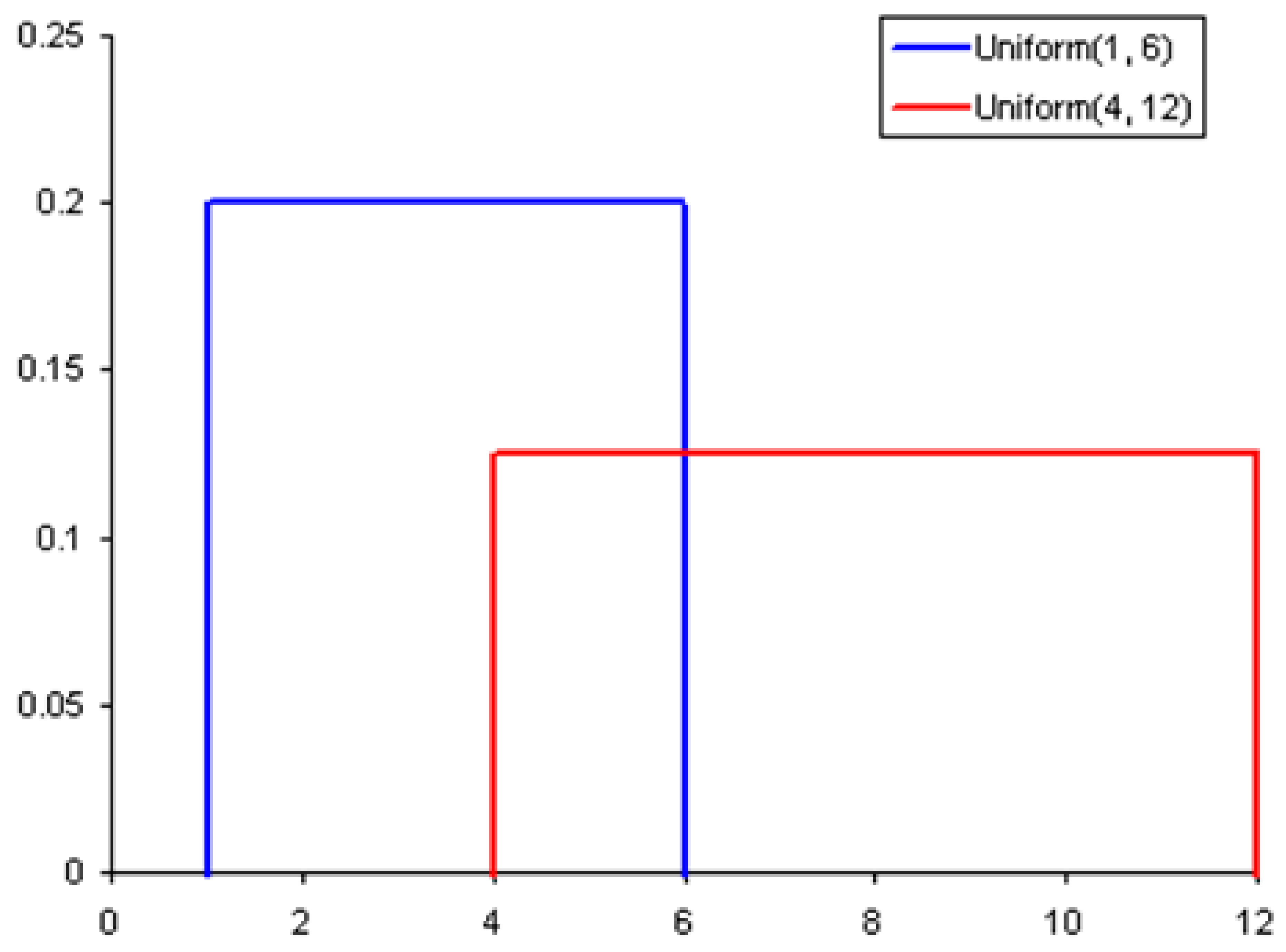
After identifying the sensitive parameters for the HOE variables, a Monte Carlo simulation (1000 runs) was performed (see Appendix E for description of procedures on SD sensitivity analysis). The Vensim tool for Monte Carlo simulation provides the 50th, 75th, 95th and 100th percentile confidence interval bounds of the simulations and according to [39], these intervals can be approximated as the corresponding confidence bounds for uncertainty. The fire ignition probability variable is associated with a uniform probability distribution, with upper and lower values 0.4 and 0.3 for apartment fire (0.384-point value) and 0.02 and 0.01 for corridor fire (0.0198-point value). This distribution was chosen to characterize uncertainty in non-calibrated uncertain parameters varied in the Monte Carlo simulations. 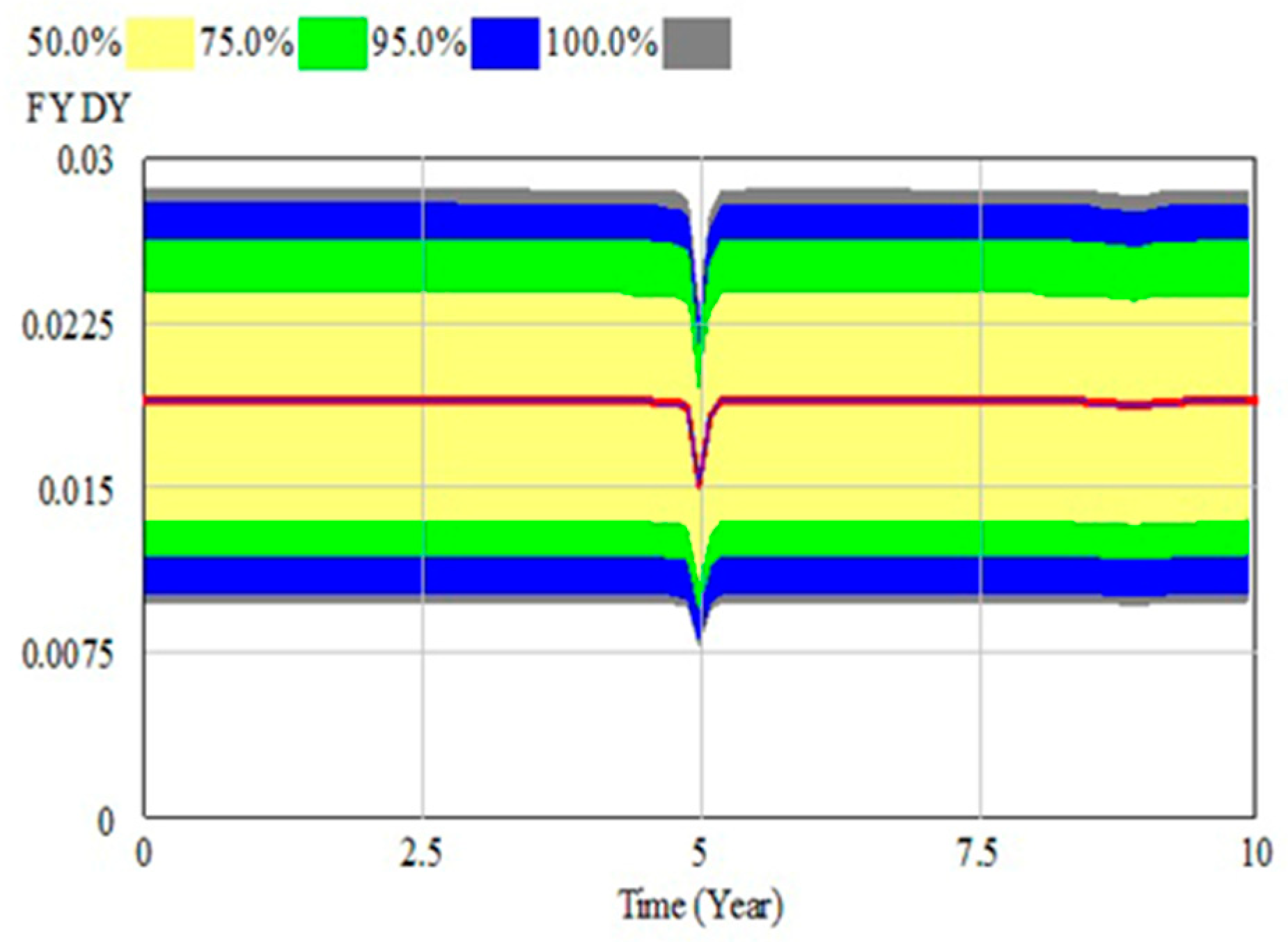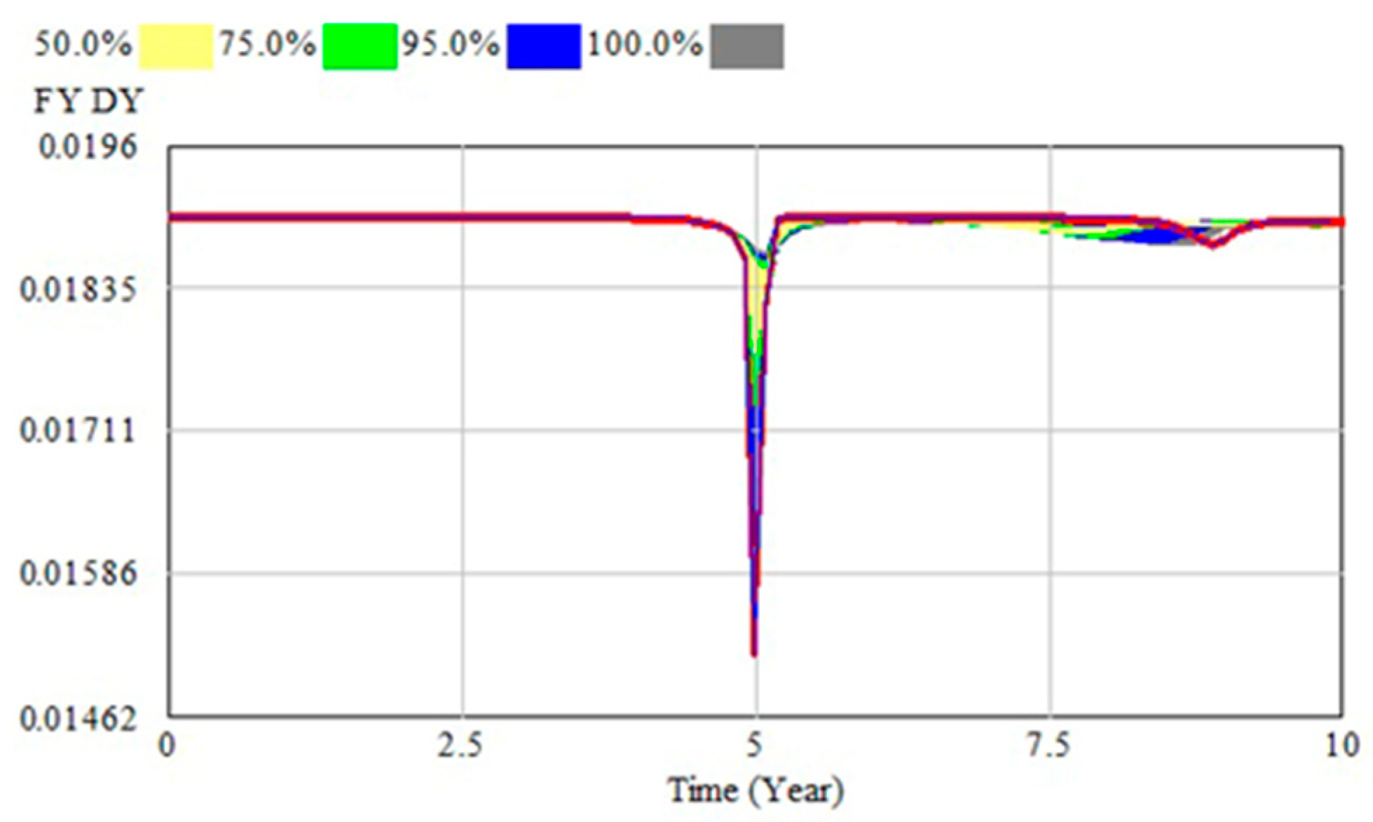Figure 22 represents the variation of the ‘fire yes detection yes node’ (FYDY node) with fire ignition frequency. The FYDY node expresses the frequency of fire ignition and subsequent fire detection. As expected, the relationship between the two variables is linear and the SD curve is shifted upward when fire ignition probability increases and downward when fire ignition decreases. Moreover, this relationship remains constant with time.

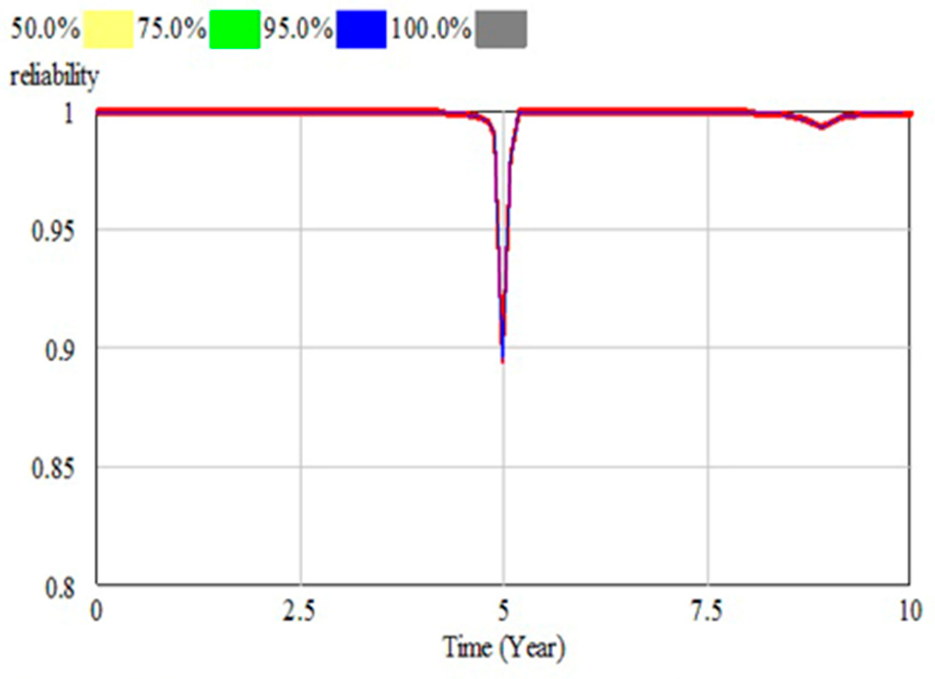
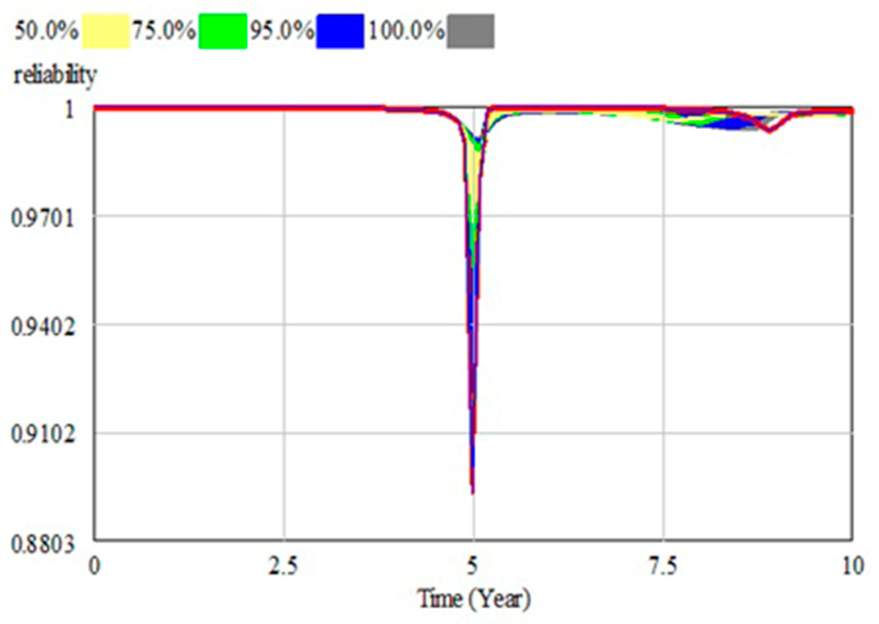
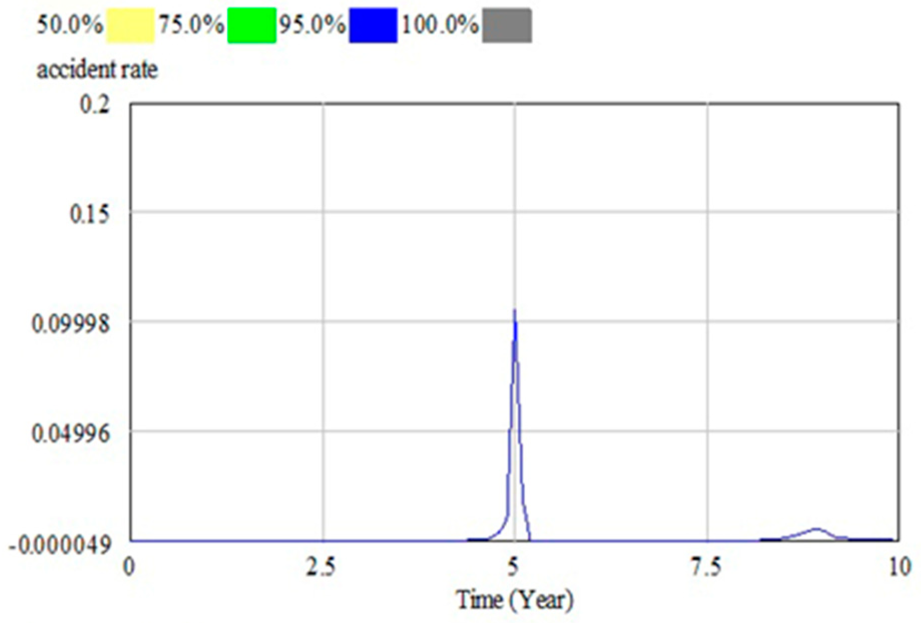
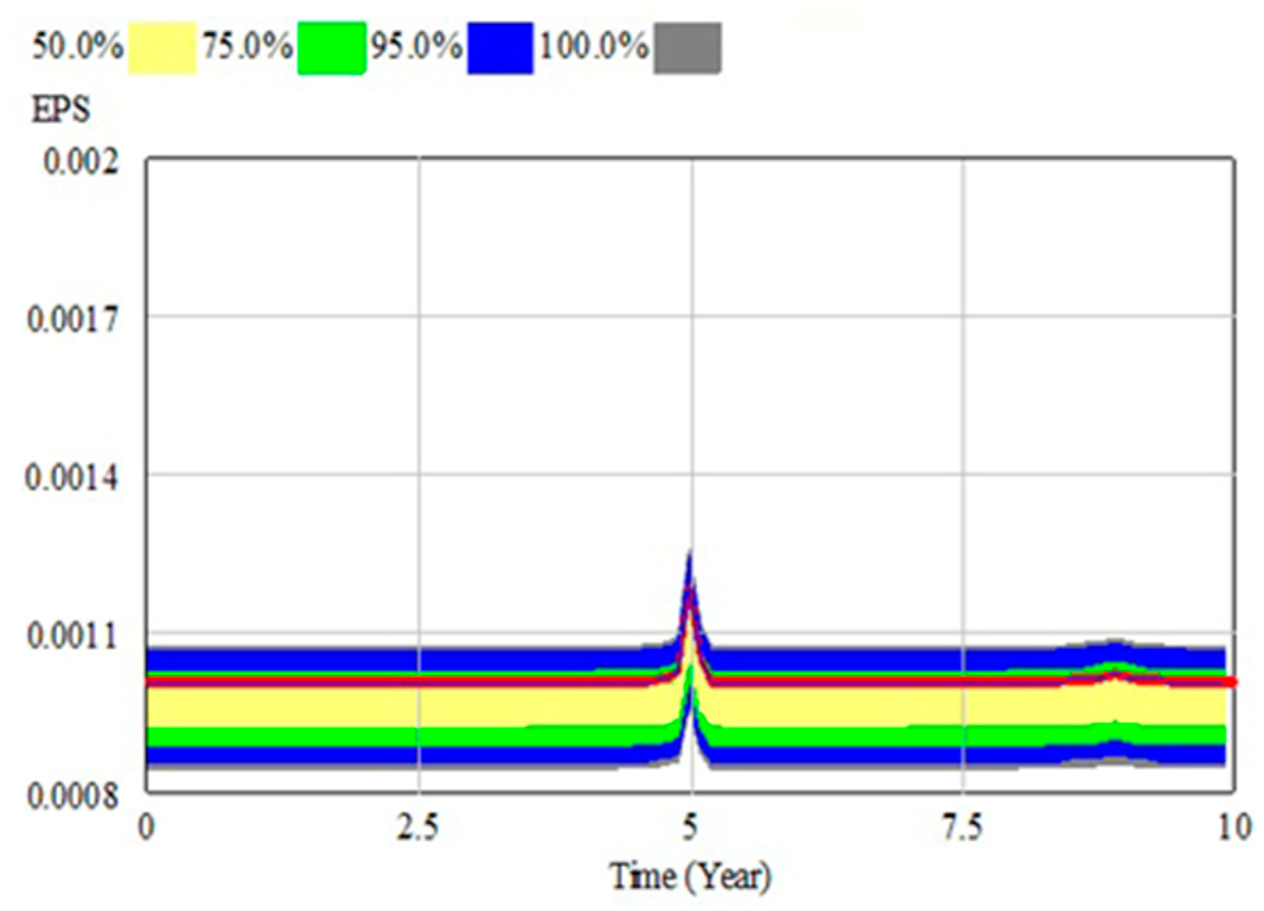
Another important variable, ‘reliability’, is not affected by the fire ignition frequency (see Figure 23). Given the fact that after a fire event all safety systems are properly checked, it can be safely assumed that their efficacy is not determined by the number of previous activations. The same observations can be made for the loop variable ‘accident rate’ as shown in Figure 24. In Figure 25, the ERL varies linearly with the fire ignition frequency. Sensitivity is not affected here by dynamic behaviours.

To determine sensitivity of the model to HOE variables, the parameter ‘Probability of valve left closed’ was analysed. A triangular probability is associated with the variable, with values comprised from 0.01 to 0.015 (min = 0, max = 0.5, start = 0.01, peak = 0.01, stop = 0.015). The resulting curve for the reliability parameter is shown in Figure 26. It can be argued that the reference curve (in red) is smoothened by variations in the HOE variable. The fall in reliability is always below the static values at year five for the ‘Probability of left valve closed’ ranging from 0.01 to 0.015.

Similar observations can be made from the ‘detection’ node as shown in Figure 27. From the results it can be observed that the impact of the fire ignition frequency is greater than all other variables and the correlation is not linear as different variations occur at different time steps.

4.5. Assessment of Robustness of SD Model Outputs

The outputs of the SD model are tested for robustness by screening the variables to identify and select the most sensitive parameters for each target variable in the model. Monte Carlo simulations were performed (one for each target variable) to establish the confidence intervals (CI) for outputs responding to sensitive variables. The variation coefficient VC_i,t of the target variables was calculated for ten years based on the following equation:

$$V{C}_{i,t}=\left(\frac{OM{95}_{i,t }– Om{95}_{i,t}}{O_i^m}\right)\times 100$$

(6)

where VC_i,t is relative variation of target variable I with respect to the mean using 95% CI; OM95_i,t and Om95_i,t are max. & min. values of the ith target variable at time t, using the 95% CI; and O_i^m is mean value of target variable i. There are 3 categories of response: low where VCi is less than 50%, moderate where variation coefficient is between 50–100% and high where variation coefficient is higher than 100%

First, for each of the three responsive parameters (i.e., perception, number of accident and probability valve closed) a univariate analysis is performed to assess the sensitivity of the following target variables: deficient training, inefficient emergency plan, not comply with instruction, no check rules, deficient maintenance, wrong risk assessment, not obey standard and improper safety organization. A uniform distribution was applied. In this way, it is possible to characterize which variables are more sensitive to organizational response.

The analysis shows that the influence of the parameter ‘Perception’ is high for ‘Inefficient timely control’ and ‘Not comply with instructions’ target variables, with values above the 100% sensitivity. ‘Improper safety organisation’, ‘Inefficient emergency plan’, ‘No check rules’ and ‘Not obey standards’ presents a sensitivity between 50% and 100%, Finally, ‘adopt unsuitable equipment’ is insensitive to the variation of the ‘Perception’ parameter, with a sensitivity value of about 1%. The ‘Max number of accidents’ parameter has little influence on the HOE variables, with values in the range between 0.1% and 23%. Finally, the variable ‘Probability Valve Closed’ has the lowest impact, in the range from 0.1 to 11. In general, it can be observed that the variable ‘Perception’ is by far the most impacting factor and the target variables of ‘Inefficient timely control’ and ‘Not comply with instruction’ are much more sensitive to variation of the reference parameters than the other variables.

As multivariate analysis is used to assess the robustness of the model and to define the ranges of variations of the target variable. Results are reported in

Table 8. Results of Monte Carlo Sensitivity analysis of responsive parameters.

Target Model Variables	Responsive Parameters	Sensitivity Results 95% Confidence Interval
Adopt unsuitable equipment:	Perception, Max number of accidents, Probability Valve Closed	0.92 ± 0.004 (dimensionless)
Improper safety organisation	Perception, Max number of accidents, Probability Valve Closed	1.29 ± 0.233 (dimensionless)
Inefficient timely control	Perception, Max number of accidents, Probability Valve Closed	0.25 ± 0.212 (dimensionless)
Inefficient emergency plan	Perception, Max number of accidents, Probability Valve Closed	1.24 ± 0.226 (dimensionless)
No check rules	Perception, Max number of accidents, Probability Valve Closed	0.29 ± 0.211 (dimensionless)
Not comply with instructions	Perception, Max number of accidents, Probability Valve Closed	0.30 ± 0.219 (dimensionless)
Not obey standards	Perception, Max number of accidents, Probability Valve Closed	1.29 ± 0.236 (dimensionless)

and sensitivity of some variables are shown in Figure 28. See Appendix F

Table A6. List of parameters in System Dynamics model.

Parameters	Model Value (Units)	Definition/Equation	Range of Variation (Multi)
adopt unsuitable equipment	dimensionless	1 − (improper safety organisation yes) × (1 − dump1 × not obey standards)	0.0028–0.0048
fire probability	dimensionless	ignition frequency + RANDOM UNIFORM(−default Change/4, default Change/4, 1) × ignition frequency	0.0023–0.0038
inefficient emergency control plan	dimensionless	1 − (1 − deficient training yes) × (1 − dump2 × not comp w instr yes) × (1 − control2 × inefficient emergency plan yes)	0.0053–0088
not obey standards	dimensionless	1.05 − Level of organisation/4	0.16–0.28
wrong risk assessment	dimensionless	1.3 − Level of organisation/4	0.48–0.58
deficient check	dimensionless	1 − deficient check no	0.23–0.45
deficient maintenance	dimensionless	deficient maintenance = RANDOM UNIFORM(− default Change, default Change, 1) × deficient maintenance yes	0.06–0.10
deficient training	dimensionless	1 − Level of organization	0.0645–0.1075
electrical failure	dimensionless	1 − (1 − component faulty connection) × (1 − no battery)	0.0375–0.0625
equipment aging	dimensionless	1 − (deficient maintenance yes a)*(1 − wrong risk assessment)	0.2325–0.3875
improper safety organisation	dimensionless	1.3 − control4 × Level of organisation/4	0.075–0.125
inefficient timely control	dimensionless	1 − (deficient training yes) × (1 − dump2 × not comp w instr yes) × (1 − control3 × inefficient emergency plan)	0.315–0.525
inefficient emergency plan	dimensionless	1.25 − Level of organisation*dump5/4	0.092–0.154
Level of organisation	dimensionless	rate of change	1 to 4
n° of accidents	dimensionless	INTEG(accident rate)	15–25
no check rules	dimensionless	1.3 − Level of organisation*dump6/4	0.1065–0.1775
not comply with instructions	dimensionless	0.3 + deficient training	0.3045–0.5075
Number of checks	number per year	INTEG(rate of change)	23.25–38.75
perceived safety	dimensionless	gap in no of accidents × perception	2.175–3.625
ProbCheckFailure	dimensionless	0.4 × deficient training + 0.1	0.0825–0.1375
ProbValveClosed	dimensionless	ProbValveClosed = 0.01 + RAMP(0.05,1,20)	0.0075–0125
reliability	days/year	1 − (((ProbCheckFailure × 19) + 1)/20) + ProbValveClosed a + (1/N° of checks)	9 to 15
smoke alarm failure	dimensionless	1 − (1 − panel failure) × 1 − zone isolated)	0.675–0.925
notification failure	dimensionless	1 − (1 − bell failure) × (1 − bulb failure)	0.75–0.95
panel failure	dimensionless	1 − (1 − electronic failure)*(1 − notification failure)	0.011175–0.018625
sprinkler failure	dimensionless	Probability of Failure on Demand (PFD) [43,48]	0.85–0.95
sprinkler head failure	dimensionless	Probability of Failure on Demand (PFD) [43,48]	0.00225–0.0375
water supply failure	dimensionless	Probability of Failure on Demand (PFD) [43,48]	0.099–0.165
downfeed failure	dimensionless	Probability of Failure on Demand (PFD) [43,48]	0.019725–0.032875
pressure valve failure	dimensionless	Probability of Failure on Demand (PFD) [43,48]	0.00093–0.00155
outlet valve failure	dimensionless	Probability of Failure on Demand (PFD) [43,48]	0.000465–0.000775
isolation closed	dimensionless	Probability of Failure on Demand (PFD) [43,48]	0.0174–0.029
water valve closed	dimensionless	Probability of Failure on Demand (PFD) [43,48]	0.001425–0.002375
pressure valve closed	dimensionless	Probability of Failure on Demand (PFD) [43,48]	0.000472–000788
tank failure	dimensionless	Probability of Failure on Demand (PFD) [43,48]	0.08175–0.13625
pump failure	dimensionless	Probability of Failure on Demand (PFD) [43,48]	0.0423–0.0705
return valve closed	dimensionless	Probability of Failure on Demand (PFD) [43,48]	0.0009–0.0015
operator fails	dimensionless	Probability of Failure on Demand (PFD) [43,48]	0.0009–0.0015
flow probability	dimensionless	Probability of Failure on Demand (PFD) [43,48]	0.70–0.90
valve left closed	dimensionless	Probability of Failure on Demand (PFD) [43,48]	0.0009–0015
alarm valve	dimensionless	Probability of Failure on Demand (PFD) [43,48]	0.00141–00235
ordinary stop valve	dimensionless	Probability of Failure on Demand (PFD) [43,48]	0.000465–000775
non-return valve	dimensionless	Probability of Failure on Demand (PFD) [43,48]	0.0008925–001488
alarm bell	dimensionless	Probability of Failure on Demand (PFD) [43,48]	0.02175–0.03625
storage tank	dimensionless	Probability of Failure on Demand (PFD) [43,48]	0.0054225–0.009038
mains power	dimensionless	Probability of Failure on Demand (PFD) [43,48]	0.0002745–0.000458
pressure switch	dimensionless	Probability of Failure on Demand (PFD) [43,48]	0.0059175–0.009863
diesel pump	dimensionless	Probability of Failure on Demand (PFD) [43,48]	0.069–0.115

for list of parameters:

Results from this analysis indicate that all targets show similar ranges of variations around their own average value, except ‘Adopt unsuitable equipment’ which has a very low variability of 0.04. The results of the MC simulations show that all the target variables exhibit either a low or moderate response to changes in the responsive parameters. This indicates a high degree of robustness in the SD model and hence, the model outcomes can be accepted with confidence.

5. Conclusions

Summary: The current study demonstrates how T-H-O-Risk methodology enhances current FSVMs by incorporating HOEs in a PRA for a more inclusive view of risk in high-rise residential buildings. The limitations of existing deterministic methods and how they are overcome using the T-H-O-risk methodology is elaborated in this paper. While the T-H-O-risk approach enables an integrated analysis of HOE factors and their nonlinear interactions and feedbacks, it generally results in a higher level of uncertainty, hence, detailed sensitivity and uncertainty analyses were performed to assess the model robustness and reliability of model outputs.

Influence of HOEs: The study identifies the most important HOE variables and the extent they contribute to the fire risk in high-rise buildings. Uncertainties in point estimate of ERL values are propagated through appropriate probability distributions with Monte Carlo simulations while a family of F-N curves propagate epistemic uncertainty in societal risks of the case studies. Four case studies were used for the study including the reference case from the ABCB FSVM Handbook. For each case, a performance solution, a performance solution incorporating HOEs and a DTS solution were compared using risk values that assess the level of safety. The analysis finds that the level of risk as measured by the ERL of the performance solution is lower than the DTS solution however when HOEs are considered, their influence is significant for all cases.

Sensitivity and uncertainty analyses—A sensitivity analysis using a Monte Carlo approach found that the most influential HOE variables were ‘not complying with instructions’, ‘deficient training’ and ‘inefficient emergency plan’. An uncertainty analysis of the ERL indicates that the most influencing HOE factors determine important variations in the ERL value of the system by up to 30% of the reference value. The minimum amount of variation associated with these HOEs is approximately 3–5% indicating that HOEs impact global risk levels; the F-N curves for all cases and scenarios with HOEs shift upwards indicating risk is underestimated when HOEs are ignored. Indeed, as system complexity increases, so does the influence of HOEs on risk primarily due to increasing numbers of fire safety measures and maintenance regimes. Sensitivity and uncertainty analyses in SD risk modelling indicate that risk thresholds oscillate or spike at year seven over the 10-year cycle. Risk variation over time analysis indicates that maintenance of an active safety system is required within five to seven years due to the degrading influence of HOEs on the reliability of the system.

Advantages of T-H-O-Risk—The research demonstrates how fire safety verification methods can be improved with the incorporation of human and organizational risks in PRA, where uncertainties in point estimates of individual risk are propagated with probability distributions while uncertainties in societal risks and risk variations over time due to human and organizational risks are propagated with confidence-interval-based societal risk curves. It is important to determine the significance of uncertainty in the PRA process, to produce effective fire safety measures for high-rise residential buildings.

State-of-the-art PRA—Although there are instances of using HOEs for modelling in other applications and industries, this is the first state-of-the-art methodology where HOEs have been incorporated in the fire risk analysis for high-rise buildings in a comprehensive manner, where technical systems such as sprinklers and smoke detection systems are integrated with HOEs. When HOEs are ignored in a PRA, overall risk levels are likely to be underestimated given that some DTS or performance-based designs that were initially assessed as within an ALARP region may fail the tolerability limit when HOEs are included. Hence, HOE variables will need to be considered when performing a Cost–benefit Analysis. The risk is not only quantified with the T-H-O-Risk approach, but the methodology also pinpoints various parameters that need to be controlled to minimize risk. Existing methods do not provide any empirical relations in predicting risks for different HOE parameters, making the T-H-O-Risk methodology even more significant.

Contribution—The T-H-O-Risk model contributes to the existing knowledge base related to risk modelling and the incorporation of HOEs in those models. This effort fills an existing gap in the literature and in existing fire risk models that fail to include and quantify the impact of HOEs. By incorporating BN and SD techniques, the enhanced model addresses HOEs dynamically in an innovative and integrated quantitative risk framework. This integrated modelling approach allows for a broader understanding of technical, human, and organizational risks in high-rise buildings, including a means to estimate the range of impacts that result from including these risks in the model that is lacking in current state-of-the-art models.

Policy implications—As far as policy implications are concerned, the ability to estimate the risk impacts: (a) significantly benefits stakeholders in Australia, including the ABCB, and their efforts to better quantify risk and tolerability levels as quantifying at this level means that health and safety can be clearly represented in terms of individual and societal risk and allows for flexibility in achieving these goals. (b) by incorporating individual and societal risk, fire authorities and building regulations can be proactive in their approach to events with multiple fatalities. Evaluating the frequency of events and the number of fatalities supports a quantitative (c) risk assessment (QRA) and ultimately drives risk as a basis for fire safety; (d) contributes to the development of next-generation building codes and risk assessment methodologies by demonstrating how fire safety verification methods can be improved with the incorporation of HOEs in PRA.