Abstract
In the workspace of robot manipulators in practice, it is common that there are both static and periodic moving obstacles. Existing results in the literature have been focusing mainly on the static obstacles. This paper is concerned with multi-arm manipulators with periodically moving obstacles. Due to the high-dimensional property and the moving obstacles, existing results suffer from finding the optimal path for given arbitrary starting and goal points. To solve the path planning problem, this paper presents a SAC-based (Soft actor–critic) path planning algorithm for multi-arm manipulators with periodically moving obstacles. In particular, the deep neural networks in the SAC are designed such that they utilize the position information of the moving obstacles over the past finite time horizon. In addition, the hindsight experience replay (HER) technique is employed to use the training data efficiently. In order to show the performance of the proposed SAC-based path planning, both simulation and experiment results using open manipulators are given.
1. Introduction
In the fourth industrial revolution, the operation of an autonomous multi-robot in a complicated workspace has been an important challenge for modern smart factories [1]. It is important to replace the human workforce with robots, to collaborate with robots, and to deploy robots in an efficient manner [2,3]. This paper presents a deep reinforcement learning-based path planning algorithm to deal with periodically moving obstacles.
1.1. Background and Motivation
In the autonomous robot framework, there are three fundamental concepts such as perception, planning, and control [4]. The perception aims to obtain information about the environment using various sensors. The planning schedules a sequence of valid configurations for the robot arms or wheels in order to perform a given task. When the path achieving the goal is given, the controller adjusts actuators so that, for example, the configurations of the robot manipulators follow the planned path as close as possible.
Although the robot manipulator operation is quite diverse in the workspace, most operations can simply be interpreted as moving the robot from a starting point to a goal point. Hence, it is utmost essential for the manipulator to move without collision with any obstacles in the workspace. In practice, there are typically two kinds of obstacles: static and periodically moving obstacles. In the case of static obstacles, their locations do not change in the middle of the robot operation, and most existing path planning methods focus on the static obstacles. For the robot operation with the static obstacles, it is a common situation in practice that human experts design the path for the robot manipulators in order to perform a given task. Recent research effort is directed to make this procedure in an automatic manner. In other words, the human experts’ path planning is replaced with various automatic algorithms [5]. The other is the periodically moving obstacle. For the purpose of dealing with the moving obstacles, this paper considers the situation where every dynamic object in the workspace moves by plan. Consequentially, it is assumed in this paper that there are no unexpected obstacles, and that all dynamic obstacles are moving periodically. In the case of industrial robots in a real factory, this is the case. Moreover, since one robot manipulator is viewed as an obstacle to the other robots, and the entire operation on a factory is usually batch production, many obstacles can be regarded as periodically moving obstacles if they are not static obstacles. Since existing path planning algorithms deal with such a moving obstacle using any methods for static obstacles, the results are conservative. In other words, to deal with the moving obstacles, those algorithms view the whole area where the obstacle moves as one big artificial static obstacle, which is inevitably conservative.
In robot path planning research, the sampling-based algorithm is representative [6]. In order to compute the path connecting the initial and goal points, the sampling-based algorithm samples the nodes from the collision-free space and connects those nodes. Hence, the method relies on how to sample the nodes. In the case of multi-arm manipulators, the problem dimension increases quadratically as the number of arms increases, which makes it difficult for the planner to find an optimal path. Moreover, if the obstacle moves, it is not easy to use the sampling-based algorithms. Existing path planning algorithms, especially sample-based approaches, work well for a single robot manipulator. However, if the target manipulator is a multi-arm manipulator with moving obstacles, the path planning problem becomes difficult since the problem dimension is high and it is not trivial to sample the configuration space.
Hence, the focus of this paper is placed on devising a deep reinforcement learning-based path planning algorithm which can generate collision-free paths when the multi-arm manipulator has both static and periodically moving obstacles.
1.2. Related Work
Fast marching method (FMM) [7], probabilistic road map (PRM) method [8], and rapid exploring random trees (RRT) method [9,10,11] are representatives of sampling-based algorithms. In PRM, the shortest path is computed from the graph made by the sampled points using the Dijkstra algorithm [12,13]. Artificial potential field methods are also popularly used to design the path planning algorithm which leads the robot manipulator from the starting point to the goal point [14,15]. In the derivation, the gradient of the potential function plays a key role in computing the direction of the optimal path [16]. Since it is based on the gradient descent method, it can suffer from trapping in the local minimum, which makes it difficult to be applied to high-dimensional problems [17]. In addition, artificial intelligence like reinforcement learning is also widely used to design collision-avoiding path planning [18]. In [19], Real-Time RRT* (RT-RRT*) is proposed to solve the path planning problem with a dynamic obstacle in a two-dimensional environment.
This paper improves the result in [5,20] in such a way that the deep reinforcement learning-based path planning for multi-arm manipulators with both static and periodically moving obstacles is proposed using the SAC algorithm with hindsight experience replay (HER).
1.3. Proposed Method
This paper proposes a deep reinforcement learning-based path planning algorithm for multi-arm manipulators with periodically moving obstacles. In particular, in order to deal with the high-dimensional property of the multi-arm manipulators, the SAC-based path planning algorithm is devised. Since the SAC-based algorithm uses an entropy term in its objective function, it can find the optimal solution of the high-dimensional problem, which makes the SAC-based algorithm outperform the existing results. Moreover, for the purpose of handling periodically moving obstacles in the path planning, the neural networks in the SAC are designed such that the position information of the obstacles over the past finite time horizon is used as an input to the neural networks together with the joint information of the robot. Note that the SAC employs five neural networks in order to estimate the value function and optimal policy. Hence, it is crucial to design the neural networks appropriately depending on the given problem. After the proposed SAC-based path planning is trained offline for various starting and goal points in the workspace, it can find the optimal path for arbitrary starting and goal points online by computing the forward path of the trained actor-network, which means that the proposed method is computationally cheap even for the high-dimensional problems. Both simulation and experiment results using real robot manipulators show the efficiency of the proposed method.
2. Background Concept and Problem Modeling
2.1. Path Planning for Robot Manipulator and Configuration Space
In the path planning problem for a robot manipulator, the configuration is defined as a position representation of the robot in the workspace. In other words, the configuration space (also called joint space in a robot manipulator) is a set of all possible joint angles of the robot manipulator [3,21,22]. To be specific, is defined as a subset of n-dimensional vector space , where n is the number of the joints of the robot manipulator. Because of this reason, the position of the robot can be represented as point that has n angle values (), where each value indicates the joint angle of the robot. The set consists of two subsets: the first subset is the collision-free space that is comprised of all possible configurations, and in which the robot does not collide with any obstacles or itself. The second subset is called the collision space which is the complement of in and the subset of . In , the robot arm manipulator collides with obstacles or itself [21,23]. The robot manipulator does not collide with any obstacles or itself if its joint angles belong to . However, if there is a collision between the robot manipulator and obstacles or itself, the values of the joint angles must be in .
In the sampling-based method, the discrete representation of is obtained by random sampling in . The valid path is defined by a connected line between the sampling points. Such sampled points and paths can establish a graph. Because of this construction, the nodes in the graph describe possible configurations of the robot manipulators. In addition, the collision-free paths between any two nodes are represented by connected edges in the graph. For the notation of the path planning problem, let mean the values of the joint angles of the manipulator at the tth iteration, and T describe the maximum number of iterations in the algorithm. Thus, the algorithm needs to find the path within T iterations for a given starting configuration and goal configuration .
Based on this concept, when and are acquired, the algorithm computes a valid continuous and shortest path linking and . The path is defined as a sequence of the state such that where . In addition, the sequence and the line segment connecting any two neighbors state and from have to belong to .
2.2. Collision Detection in Workspace Using the Oriented Bounding Box (OBB)
The definition of workspace is a space where an actual robot operates. In many cases including the robot manipulator, space is in three-dimensional Euclidean space . To confirm that , collision detection methods have to be applied in workspace [21,23]. To this end, the oriented bounding boxes (OBB) [24] is employed for collision detection. In OBB, both the robot arm and obstacles are modeled as a box. Because the modeling is implemented in OBB, the collision checking between 2 boxes only has 15 cases: three faces of the first box, three faces of the second box, and nine edge combinations between the first box and second box [25]. Based on two box checking, the higher level checking between one robot and one obstacle can be implemented as a repeated two OBB checking [26].
2.3. Reinforcement Learning
As a standard solution to the MDP problem, the fundamental method in the reinforcement learning algorithm uses an optimization-based method to maximize the sum of the reward signal by letting the agent interact with a stochastic environment and choose the action over sequences of discrete-time steps [27]. The MDP is defined by the tuple , where S denotes the set of the state, A the set of action, P the transition probability, the reward function, and the discount factor [28]. The transition probability represents the probability of moving the current state s to the next state when action is applied. Regarding the agent, the distribution of action a for the given state s from the environment is implied by the policy that is denoted by . At each time step t, the agent selects action based on the policy and state , and applies it to the environment. After that, the environment returns both the next state and reward according to the transition probability , where means that the probability of the next state and the reward function . By repeating this procedure, the learning process updates the policy until it reaches the optimal policy, defined by , which maximizes the expected return . In order to acquire the optimal policy, the optimal value function (i.e., estimate of the maximum return) is approximated by value-based methods like deep Q-network (DQN) as function approximation [29]. The other way to get the optimal policy is using the policy gradient methods to compute the optimal policy directly from the agent experience. Representative methods of the policy gradient are REINFORCE, actor–critic method, deterministic policy gradient (DPG), deep DPG (DDPG), asynchronous advantage actor–critic (A3C), trust region policy optimization (TRPO), maximum a posteriori policy optimization (MPO), and distributed distributional DDPG (D4PG) [30,31,32,33,34]. In the reinforcement learning, the training performance mostly depends on the set of samples of state , action , reward , and next state . In addition to the various reinforcement learning algorithms, efforts are directed at devising techniques to utilize the samples (called episode) effectively for better learning, for example replay memory [29] and HER [35]. In this paper, for the purpose of tackling the path planning problem for the multi-arm manipulators with periodically moving obstacles, a soft actor–critic (SAC)[36] algorithm is employed.
3. Soft Actor–Critic Based Path Planning for Periodically Moving Obstacles
In this section, in order to design a SAC-based path planning, the MDP for the problem is defined, and the proposed deep learning network used in the SAC is presented. Although the considered MDP is quite similar to that in [20], since both deal with multi-arm manipulators, the MDP is explained here in a self-contained manner.
3.1. Path Planning for the Multi-Arm Manipulator and Augmented Configuration Space
The multi-arm manipulator under consideration consists of m identical robot-arm manipulators that have n number of joints. Let determine the joint angles of the ith robot-arm at the tth iteration in the proposed SAC-based method, and denotes the jth component of , i.e., the value of the jth joint angle of the ith robot-arm.
In the path planning algorithm for the multi-arm manipulator, if the configuration space is defined for each robot, it is difficult to define and during the robot operation since for each arm is affected by the other arms, i.e., one robot serves as an obstacle to the others in the workspace. Taking this into account, it is convenient to define one big configuration space by augmenting the configuration space of each manipulator. This corresponds to regarding the multi-arm manipulator as one virtual manipulator. The dimension of the augmented configuration space is . Hence, the state of the virtual manipulator is represented by
Therefore, the resulting augmented configuration space is described by where
defines the collision-free space for and denotes the corresponding collision space. Finally, the path planning problem of the multi-arm manipulator can be redefined as the path planning for the (virtual) single-arm manipulator with a given starting point and goal point being
where and denote the starting and goal point of the ith robot-arm.
3.2. Multi-Arm Manipulator Markov Decision Process Considering Periodically Moving Obstacle
In order to apply deep reinforcement learning to the path planning algorithm for the multi-arm manipulator considering a periodically moving obstacle, a multi-arm manipulator MDP (MAMMDP), i.e., the tuple , needs to be defined. For a better understanding, the diagram of MAMMDP is depicted in Figure 1.
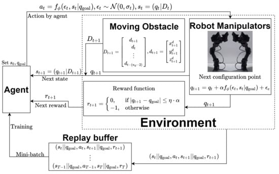
Figure 1.
Multi-arm manipulator MDP considering periodically moving obstacle (MAMMDP).
In principle, MAMMDP is similar to MAMMDP in [20]. The only difference is that the state in MAMMDP is defined such that the information on the moving obstacle is related to the state. For this purpose, it has to be determined which information on the obstacle is used in defining MAMMDP. In this paper, the location of the obstacle in the workspace for the past sampling times is used where denotes the window size. Namely, the following information on the obstacle is used:
where represents the location of the obstacle in the workspace at the sampling time t. This can be viewed as the number of the features obtained from the obstacle. In addition to this time window, it is also assumed that is available only when the obstacle belongs to a predefined region such as a neighborhood of the multi-arm manipulator. When the manipulator does not belong to the region, is not available to the MAMMDP. With this in mind, the current state is defined as . In other words, the state contains the information of not only the current configuration of the multi-arm manipulator but also (i.e., obstacle location over the past sampling times).
The action is calculated by , where follows the Gaussian distribution with being the variance, and generates a stochastic action using noise and state . As a matter of fact, function serves as a sampler. Thus, the action is sampled from a probability distribution and variation of the configuration. Then, the next configuration is calculated as the sum of the current configuration and the action such as , where tuning parameter is defined as the geometric mean of the maximum variations of each joint and is an environmental noise, where . When happens, the next configuration becomes the previous configuration meaning that it stays at the current configuration. The following summarizes how the configuration is updated:
Using this, the next state is denoted as , where is the updated information of the obstacle position. Applying the action and obtaining the state and reward are repeated until the next configuration reaches the goal point . Owing to the practical limitation like numerical errors, instead of , the relaxed condition is employed for the termination in an implementation where defines the norm of a vector and tuning parameter satisfies .
If the next configuration is not the goal point, the corresponding reward is . However, when the agent meets the terminal condition, the corresponding reward becomes 0. If the agent cannot reach the goal until the maximum number of iteration, the total reward is given by . On the other case, if the iteration ends at a certain iteration , the total reward amounts to . This reward function is summarized as follows:
In view of the goal of reinforcement learning, the objective of the proposed algorithm is to find the optimal policy that maximizes the total reward. If the iteration can finish before reaching T, the sum of reward is more than such as . By trying to maximize the total reward in training process, the agent finds the shortest path.
In the next subsection, it is presented how to update the policy in the middle of training using deep neural networks.
3.3. Soft Actor–Critic (SAC) Based Path Planning Considering Periodically Moving Obstacles
Since our MAMMDP has a continuous action value, there are several reinforcement learning methods for continuous action MDP such as those in [32,36,37]. Soft actor–critic (SAC), especially, is the best known for its performance for the MDP with the continuous action and high-dimensional state. SAC is based on maximum entropy reinforcement learning that maximizes not only the expected sum of rewards but also the entropy of the policy of action [36,38].
When the policy is updated by maximizing only the total reward, the center of the distribution of the policy is formed around a specific action. However, by maximizing policy entropy together with the reward, the SAC method can make the distribution spread more and encourage the agent to explore a wider range of the actions. The soft state-value function and soft Q-value function are defined as follows:
where denotes the temperature parameter of the entropy function. The soft state value function defined in (4) is the expected sum of the entropy augmented reward for the given current state . In addition, the soft Q-value function or soft action-value function are defined in (5) and is the expected sum of augmented reward for a given pair of state and action .
For the purpose of estimating the soft value and Q-value functions, and finding the optimal policy, the SAC-based algorithm consists of five neural networks: two for the soft value function, two for the soft Q-functions, and one for the policy. The proposed SAC-based path planning utilizes the structure described in Figure 2. The structure is quite similar to that in [20] except for the information of the moving obstacle. As the proposed path planning has to take the periodically moving obstacle into account, it has to be decided properly how to use the obstacle information for the path planning. Since information has to be considered when the policy is trained at a given state in order for the manipulator to enable to avoid the obstacle, information is also used as the input to the network for the policy. In addition, since the policy network is affected by the value functions, as a result, all the neural networks for the proposed SAC-based path planning have to have information as an input.
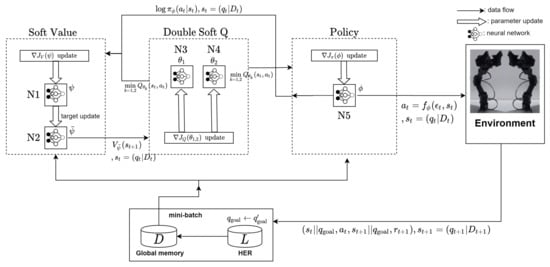
Figure 2.
Architecture of the proposed SAC-based with the HER path planning algorithm.
Figure 3 illustrates how the deep neural network (DNN) estimates the state value function. The DNNs N1 and N2 are parameterized by and . The network parameterized by is the target network which makes the training stable and enhances the learning performance of DNNs N3 and N4 for estimating the Q-value function. The inputs to DNN N1 are the configuration , goal state , and . In order to train DNN N1, the following objective function and its gradient are used:
where the minimum of the soft Q-function is determined between and , which are the output of the DNN N3 and N4. It is reported that the use of such a minimum makes it possible to avoid overestimation of Q-value [37]. The parameterized policy comes from DNN N5. To find the optimal parameter of DNN N1, the network N1 for the soft state value is trained by minimizing using . After updating the parameter using the gradient descent, the target parameter is updated according to at each training step where .
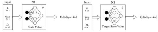
Figure 3.
The deep neural network for the state value function
In order to estimate the action value function, two DNNs are again used as depicted in Figure 4. The input to N3 and N4 are the same as those of N1 and N2. The network parameters and are trained by minimizing the following objective function:
where comes from DNN N2, and the double Q-value method is applied as it is suggested in [36,37,39]. The minimum Q-function is also used in the DNN for the objective function (8).
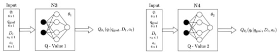
Figure 4.
The deep neural network for the action value function
Figure 5 describes the input and output of DNN N5. Similar to the other DNNs, the network parameter is trained by minimizing the objective function in the following:
where is provided by N3 and N4. In fact, this function is a kind of the Kullback–Leibler (KL) divergence between the policy and Q-value [36]. The output of DNN N5 is , and the action is sampled from such that .
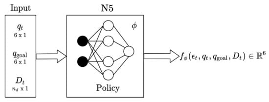
Figure 5.
The deep neural network for the policy.
Since the SAC is a type of the off-policy actor–critic method [36,40], the training gathers transition tuples in every action step and stores them in experience replay memory [29]. At the start of the training, a collection of these tuples is sampled from the reply memory and used to calculate the expectation in the objective functions. In addition to the SAC, Hindsight Experience Replay (HER) is used to enhance the sample efficiency [20,35]. In summary, the proposed SAC-based path planning algorithm is presented in the form of the pseudo-code in Algorithm 1.
| Algorithm 1 Proposed SAC-based path planning algorithm for multi-arm manipulators. |
|
4. Case Study: Two 3DOF Manipulators with a Periodically Moving Obstacle on a Line
This section presents how to implement the proposed SAC-based path training for the multi-arm manipulator with a periodically moving obstacle, and shows the result using not only simulation but also experiment.
4.1. Simulation
For the implementation of the proposed SAC-based path planning algorithm, two 3DOF open-manipulators are used. The detailed information about the manipulator can be seen at http://en.robotis.com/model/page.php?co_id=prd_openmanipulator (accessed on 14 March 2021). The entire workspace is 70 cm × 120cm × 100 cm. For the moving obstacle, a hexagon is assumed to move along a line segment back and forth periodically in the workspace, the length of the line segment is 40 cm, and the average speed of the moving obstacle is 9 cm/sec. In the simulation, it is always possible for the agent to know the location information of the obstacle. For the training, is set to 5 meaning that the location of the obstacle over the past five sampling times are given to the networks. Moreover, a square prism is located in the workspace as a static obstacle. The two manipulators are located such that the intersection of the workspace of both is not empty. The parameters of the robot manipulators and environment are summarized in Table 1.

Table 1.
Parameters of the 3DOF manipulator and environment.
The hyper-parameters of the SAC-based path planning are presented in Table 2.
Table 2.
Tuning parameters for the designed SAC with HER.
Figure 6 show the workspace under consideration. In Figure 6a, obstacle 1 moves back and forth along the line segment defined by . The obstacle 2 depicts the static obstacle. It is assumed that the manipulator 1 can detect the obstacle only when it is in , and the manipulator 2 can do only when it is in . Namely, the manipulators can detect the moving obstacle only when it is in a predefined area. In this simulation, the location of the moving obstacle is directly extracted as the input of the network. Due to that, the network can detect the obstacle location based on the input value of the network. Figure 6b describes how the PRM deals with the moving obstacle. As seen in Figure 6b, the PRM views entire as a static obstacle to deal with the moving obstacle.
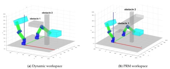
Figure 6.
The Matlab workspace.
In the learning process, the five neural networks in the proposed SAC-based path planning are trained by 70,000 episodes using GPU Nvidia GeForce RTX 2080Ti and CPU Intel i7-9700F (https://www.nvidia.com, https://www.intel.com (accessed on 14 March 2021). For the training, it took 36 h and the proposed algorithm was implemented using Tensorflow 2.1. In each episode, the agent explores and learns the environment based on the previous experience that was stored in the memory. To visualize the success of the agent, the success ratio from every 10 episodes is calculated and recorded. Figure 7 depicts the success ratio from 70,000 episodes. In Figure 7, the green chart describes the actual success ratio. However, for better visualization, the moving average of the success ratio is calculated and shown as the dark green line. At the end of the training, the success ratio reaches 81.76 %.
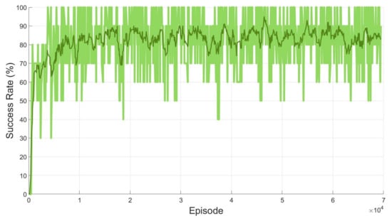
Figure 7.
Success ratio of the proposed method for two open manipulators with moving obstacles.
Not only the success ratio but also the reward value is monitored during the training. Because the agent receives −1 for the reward at every step if the next configuration is not the goal, the total reward value can be interpreted as the required total time step for the agent to complete the task. The total reward of every episode is shown in Figure 8. The light blue line tells the total reward in each episode and the dark blue line describes the moving average of the total reward. From the repeated learning, similar convergent results on the success ratio and total reward are obtained. In view of Figure 7 and Figure 8, it can be concluded that the agent is well trained, which means the agent can find the optimal path for arbitrary starting and goal configurations.
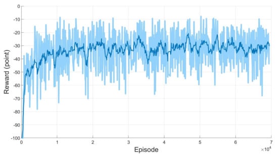
Figure 8.
Reward of the proposed SAC-based path planning for two open manipulators with moving obstacles.
In view of the learning results, the success rate of the training is not satisfactory if is set to a value less than 5. On the other hand, when it is higher than 5, the success rates of most learning reach a similar level to that with 5. This is why is set to 5. To support this, Figure 9 presents the learning performance depending on various values of .
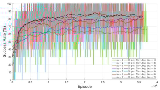
Figure 9.
Comparison of the training performance between different numbers of features.
When the training is over, the actor-network is used to generate the optimal path for an arbitrary starting and goal configurations. Figure 10 shows an example of initial and goal configurations.
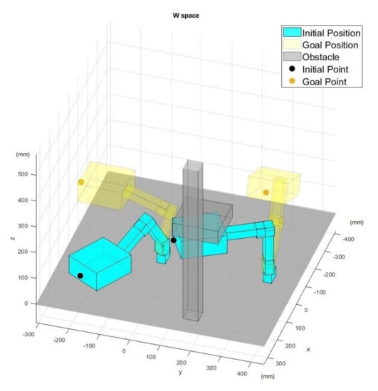
Figure 10.
Initial and goal positions in the workspace.
Figure 11 shows how the trained actor generates the path by interacting MAMMDP and measuring the location of the moving obstacle.
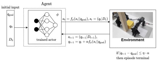
Figure 11.
Path generation using the trained actor DNN.
To be specific, () is given to the trained actor–network in the beginning and the actor–network calculates the variations of each joint denoted by in Figure 11. Then, each joint changes its angle by the variations and the resulting new configuration is generated. This is one iteration. In the second iteration, () is injected into the trained actor–network with the updated obstacle information , and the goal configuration is reached by repeating the same procedure.
One testing result is shown in Figure 12. In Figure 12, the areas in dark green denote . In this result, it is important to note that the path generated by the proposed SCA-based planning can penetrate without collision if necessary. On the other hand, the paths by other methods go around . This shows that the proposed method generates indeed an efficient path when there is a moving obstacle. For comparison, the paths computed by PRM and TD3 are also presented. Hence, there are three generated paths in Figure 12. The red lines are the resulted paths by the PRM method (10,000 sampled points graph), the blue lines by TD3 with HER, and the green lines by the proposed method path. As seen in Figure 12, the proposed SAC-based method generates the smoothest and shortest path.
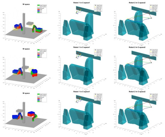
Figure 12.
Path generation by SAC with HER for Scenario 1.
To analyze quantitatively, 100 simulations with the arbitrary initial point and goal point are carried out using PRM, TD3 with HER, and the proposed method simultaneously. Then, the lengths of all 100 generated paths are given in Figure 13. As seen in Figure 13, the proposed SAC-based path planning generates the shortest path. Since, inevitably, PRM and TD3 with HER deal with the moving obstacle in a conservative manner, the result is quite natural actually. In Table 3, the optimal path by the proposed method is shorter by 14.86% than the path by PRM. If the path by the SAC with HER is compared with the path from TD3 with HER, the path by the proposed method is 17.40% better than that by TD3.
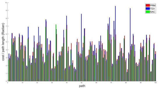
Figure 13.
Comparison of paths by PRM, TD3 with HER, and the proposed method.
Table 3.
Comparison of the proposed result with existing methods.
4.2. Experiment
In order to see if the proposed SAC-based path planning is implementable in real manipulators, it is tested using two open manipulators. Figure 14 shows the real experimental setup. In real implementation, a camera is used to detect the location of the moving obstacle and installed on the top of the workspace. The location of the moving obstacle is sampled every 0.35 s using the camera. The simulation and experimental results are displayed on the webpage https://sites.google.com/site/cdslweb/publication/dynamicsacpath (accessed on 14 March 2021). In view of the experimental results, it is confirmed that the proposed SAC-based path planning works in real multi-arm manipulators effectively.
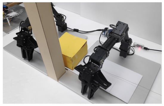
Figure 14.
The experiment using Two Open-manipulators.
5. Conclusions
This paper presents a deep reinforcement learning-based path planning algorithm for multi-arm manipulators with both static and periodically moving obstacles. To this end, the recently developed soft actor–critic (SAC) is employed for the deep reinforcement learning since the SAC can compute the optimal solution for the high-dimensional problem and the path planning problem for the multi-arm manipulators is essentially high dimensional. To be specific, the Markov decision process is properly defined for the path planning problem, and the input and output structure of the neural networks in the SAC is designed such that the information of the moving obstacles plays an important role in the training of the neural networks. In both the simulation and experimental results, it is confirmed that the proposed SAC-based path planning generates shorter and smoother paths compared with existing results when there is a periodically moving obstacle.
The role of the neural networks in the SAC is to estimate the future location of the moving obstacles. If the obstacle moves periodically, it might be possible to estimate the future location better using other deep learning algorithms tailored to estimation of the periodic signals like Recurrent Neural Networks (RNN). Hence, possible future research includes how to improve the estimation of the moving obstacle using deep learning algorithms for better path planning.
Author Contributions
E.P. surveyed the backgrounds of this research, designed the deep learning network, and performed the simulations and experiments to show the benefits of the proposed method. J.-H.P., J.-H.B. and J.-S.K. supervised and supported this study. All authors have read and agreed to the published version of the manuscript.
Funding
This work was supported by the Technology Innovation Program (or Industrial Strategic Technology Development Program) (20005024, Development of intelligent robot technology for object recognition and dexterous manipulation in the real environment) funded by the Ministry of Trade, Industry & Energy (MOTIE, Korea), and by Basic Science Research Program through the National Research Foundation of Korea (NRF) funded by the Ministry of Education (NRF-2019R1A6A1A03032119).
Conflicts of Interest
The authors declare no conflict of interest.
Abbreviations
The following abbreviations are used in this manuscript:
| MAMMDP | Multi-Arm Manipulator Markov Decision Process |
| SAC | Soft Actor–Critic |
| HER | Hindsight Experience Replay |
| AI | Artificial Intelligence |
| FMMs | Fast Marching Methods |
| PRM | Probabilistic Road Map |
| RRT | Rapid exploring Random Trees |
| DNN | Deep Neural Network |
| TD3 | Twin Delayed Deep Deterministic Policy Gradient |
| MDP | Markov Decision Process |
| DOF | Degree of Freedom |
| OBB | Oriented Bounding Boxes |
| DQN | Deep Q-Network |
| DPG | Deterministic Policy Gradient |
| DDPG | Deep Deterministic Policy Gradient |
| A3C | Asynchronous Advantage actor–critic |
| TRPO | Trust Region Policy Optimization |
| MPO | Maximum a Posteriori Policy Optimisation |
| D4PG | Distributed Distributional Deep Deterministic Policy Gradient |
| KL | Kullback–Leibler |
References
- Berman, S.; Schechtman, E.; Edan, Y. Evaluation of automatic guided vehicle systems. Robot. Comput. Integr. Manuf. 2009, 25, 522–528. [Google Scholar] [CrossRef]
- Spong, M.; Hutchinson, S.; Vidyasagar, M. Robot Modeling and Control; Institute of Electrical and Electronics Engineers Inc.: New York, NY, USA, 2006; Volume 26. [Google Scholar]
- Latombe, J.C. Robot Motion Planning; Kluwer Academic Publishers: New York, NY, USA, 1991. [Google Scholar]
- Pendleton, S.; Andersen, H.; Du, X.; Shen, X.; Meghjani, M.; Eng, Y.; Rus, D.; Ang, M. Perception, Planning, Control, and Coordination for Autonomous Vehicles. Machines 2017, 5, 6. [Google Scholar] [CrossRef]
- Kim, M.; Han, D.K.; Park, J.H.; Kim, J.S. Motion Planning of Robot Manipulators for a Smoother Path Using a Twin Delayed Deep Deterministic Policy Gradient with Hindsight Experience Replay. Appl. Sci. 2020, 10, 575. [Google Scholar] [CrossRef]
- Karaman, S.; Frazzoli, E. Sampling-based algorithms for optimal motion planning. Int. J. Robot. Res. 2011, 30, 846–894. [Google Scholar] [CrossRef]
- Janson, L.; Schmerling, E.; Clark, A.; Pavone, M. Fast marching tree: A fast marching sampling-based method for optimal motion planning in many dimensions. Int. J. Robot. Res. 2015, 34, 883–921. [Google Scholar] [CrossRef] [PubMed]
- Gharbi, M.; Cortés, J.; Simeon, T. A sampling-based path planner for dual-arm manipulation. In Proceedings of the 2008 IEEE/ASME International Conference on Advanced Intelligent Mechatronics, Xi’an China, 2–5 July 2008; pp. 383–388. [Google Scholar]
- LaValle, S.M.; Kuffner, J.J. Rapidly-exploring random trees: Progress and prospects. Algorithmic Comput. Robot. New Dir. 2001, 5, 293–308. [Google Scholar]
- Preda, N.; Manurung, A.; Lambercy, O.; Gassert, R.; Bonfè, M. Motion planning for a multi-arm surgical robot using both sampling-based algorithms and motion primitives. In Proceedings of the 2015 IEEE/RSJ International Conference on Intelligent Robots and Systems (IROS), Hamburg, Germany, 28 September–2 October 2015; pp. 1422–1427. [Google Scholar]
- Kurosu, J.; Yorozu, A.; Takahashi, M. Simultaneous Dual-Arm Motion Planning for Minimizing Operation Time. Appl. Sci. 2017, 7, 1210. [Google Scholar] [CrossRef]
- Kavraki, L.E.; Latombe, J.C.; Motwani, R.; Raghavan, P. Randomized Query Processing in Robot Path Planning. In Proceedings of the Twenty-Seventh Annual ACM Symposium on Theory of Computing, Las Vegas, NV, USA, 29 May 1995; Association for Computing Machinery: New York, NY, USA, 1995; pp. 353–362. [Google Scholar]
- Hsu, D.; Latombe, J.C.; Kurniawati, H. On the Probabilistic Foundations of Probabilistic Roadmap Planning. Int. J. Robot. Res. 2006, 25, 627–643. [Google Scholar] [CrossRef]
- De Santis, A.; Albu-Schaffer, A.; Ott, C.; Siciliano, B.; Hirzinger, G. The skeleton algorithm for self-collision avoidance of a humanoid manipulator. In Proceedings of the 2007 IEEE/ASME International Conference on Advanced Intelligent Mechatronics, Zurich, Switzerland, 4–7 September 2007; pp. 1–6. [Google Scholar]
- Dietrich, A.; Wimböck, T.; Täubig, H.; Albu-Schäffer, A.; Hirzinger, G. Extensions to reactive self-collision avoidance for torque and position controlled humanoids. In Proceedings of the 2011 IEEE International Conference on Robotics and Automation, Shanghai, China, 9–13 May 2011; pp. 3455–3462. [Google Scholar]
- Sugiura, H.; Gienger, M.; Janssen, H.; Goerick, C. Real-Time Self Collision Avoidance for Humanoids by means of Nullspace Criteria and Task Intervals. In Proceedings of the 2006 6th IEEE-RAS International Conference on Humanoid Robots, Genova, Italy, 4–6 December 2006; pp. 575–580. [Google Scholar]
- Martínez, C.; Jiménez, F. Implementation of a Potential Field-Based Decision-Making Algorithm on Autonomous Vehicles for Driving in Complex Environments. Sensors 2019, 19, 3318. [Google Scholar] [CrossRef] [PubMed]
- Sangiovanni, B.; Rendiniello, A.; Incremona, G.P.; Ferrara, A.; Piastra, M. Deep Reinforcement Learning for Collision Avoidance of Robotic Manipulators. In Proceedings of the 2018 European Control Conference (ECC), Limassoln, Cyprus, 12–15 June 2018; pp. 2063–2068. [Google Scholar]
- Naderi, K.; Rajamäki, J.; Hämäläinen, P. RT-RRT*: A Real-Time Path Planning Algorithm Based on RRT*. In Proceedings of the 8th ACM SIGGRAPH Conference on Motion in Games, Paris, France, 16–18 November 2015; Association for Computing Machinery: New York, NY, USA, 2015; pp. 113–118. [Google Scholar]
- Prianto, E.; Kim, M.; Park, J.H.; Bae, J.H.; Kim, J.S. Path Planning for Multi-Arm Manipulators Using Deep Reinforcement Learning: Soft Actor—Critic with Hindsight Experience Replay. Sensors 2020, 20, 5911. [Google Scholar] [CrossRef] [PubMed]
- Choset, H.M.; Hutchinson, S.; Lynch, K.M.; Kantor, G.; Burgard, W.; Kavraki, L.E.; Thrun, S.; Arkin, R.C. Principles of Robot Motion: Theory, Algorithms, and Implementation; MIT Press: Cambridge, MA, USA, 2005. [Google Scholar]
- Lozano-Perez. Spatial Planning: A Configuration Space Approach. IEEE Trans. Comput. 1983, C-32, 108–120. [CrossRef]
- Laumond, J.P.P. Robot Motion Planning and Control; Springer: Berlin/Heidelberg, Germany, 1998. [Google Scholar]
- Bergen, G.V.D.; Bergen, G.J. Collision Detection, 1st ed.; Morgan Kaufmann Publishers Inc.: San Francisco, CA, USA, 2003. [Google Scholar]
- Ericson, C. Real-Time Collision Detection; CRC Press, Inc.: Boca Raton, FL, USA, 2004. [Google Scholar]
- Fares, C.; Hamam, Y. Collision Detection for Rigid Bodies: A State of the Art Review. GraphiCon 2005. Available online: https://https://www.graphicon.org/html/2005/proceedings/papers/Fares.pdf (accessed on 19 August 2019).
- Puterman, M.L. Markov Decision Processes: Discrete Stochastic Dynamic Programming, 1st ed.; John Wiley & Sons, Inc.: Hoboken, NJ, USA, 1994. [Google Scholar]
- Sutton, R.S.; Barto, A.G. Reinforcement Learning: An Introduction; A Bradford Book: Cambridge, MA, USA, 2018. [Google Scholar]
- Mnih, V.; Kavukcuoglu, K.; Silver, D.; Rusu, A.A.; Veness, J.; Bellemare, M.G.; Graves, A.; Riedmiller, M.; Fidjeland, A.K.; Ostrovski, G.; et al. Human-level control through deep reinforcement learning. Nature 2015, 518, 529–533. [Google Scholar] [CrossRef] [PubMed]
- Sutton, R.S.; McAllester, D.; Singh, S.; Mansour, Y. Policy Gradient Methods for Reinforcement Learning with Function Approximation. In Proceedings of the 12th International Conference on Neural Information Processing Systems (NIPS’99), Denver, CO, USA, 29 November–4 December 1999; MIT Press: Cambridge, MA, USA, 1999; pp. 1057–1063. [Google Scholar]
- Silver, D.; Lever, G.; Heess, N.; Degris, T.; Wierstra, D.; Riedmiller, M. Deterministic Policy Gradient Algorithms. In Proceedings of the 31st International Conference on International Conference on Machine Learning, Beijing, China, 21–26 June 2014; Volume 32, pp. I–387–I–395. [Google Scholar]
- Lillicrap, T.P.; Hunt, J.J.; Pritzel, A.; Heess, N.; Erez, T.; Tassa, Y.; Silver, D.; Wierstra, D. Continuous Control with Deep Reinforcement Learning. arXiv 2016, arXiv:1509.02971. [Google Scholar]
- Abdolmaleki, A.; Springenberg, J.T.; Tassa, Y.; Munos, R.; Heess, N.; Riedmiller, M. Maximum a Posteriori Policy Optimisation. arXiv 2018, arXiv:1806.06920. [Google Scholar]
- Barth-Maron, G.; Hoffman, M.W.; Budden, D.; Dabney, W.; Horgan, D.; Dhruva, T.; Muldal, A.; Heess, N.; Lillicrap, T. Distributed Distributional Deterministic Policy Gradients. arXiv 2018, arXiv:1804.08617. [Google Scholar]
- Andrychowicz, M.; Wolski, F.; Ray, A.; Schneider, J.; Fong, R.; Welinder, P.; McGrew, B.; Tobin, J.; Pieter Abbeel, O.; Zaremba, W. Hindsight Experience Replay. In Advances in Neural Information Processing Systems 30; Curran Associates, Inc.: Red Hook, NY, USA, 2017; pp. 5048–5058. [Google Scholar]
- Haarnoja, T.; Zhou, A.; Abbeel, P.; Levine, S. Soft actor–critic: Off-Policy Maximum Entropy Deep Reinforcement Learning with a Stochastic Actor. In Proceedings of the International Conference on Machine Learning, Stockholm, Sweden, 10–15 July 2018; pp. 1861–1870. [Google Scholar]
- Fujimoto, S.; Hoof, H.; Meger, D. Addressing Function Approximation Error in actor–critic Methods. In Proceedings of the International Conference on Machine Learning, Stockholm, Sweden, 10–15 July 2018; pp. 1582–1591. [Google Scholar]
- Haarnoja, T.; Tang, H.; Abbeel, P.; Levine, S. Reinforcement Learning with Deep Energy-Based Policies. In Proceedings of the 34th International Conference on Machine Learning, Sydney, Australia, 6–11 August 2017; Volume 70, pp. 1352–1361. [Google Scholar]
- Hasselt, H.V. Double Q-learning. In Advances in Neural Information Processing Systems; Curran Associates, Inc.: Red Hook, NY, USA, 2010; pp. 2613–2621. [Google Scholar]
- Degris, T.; White, M.; Sutton, R. Off-Policy actor–critic. In Proceedings of the 29th International Conference on Machine Learning, Edinburgh, UK, 26 June–1 July 2012; Volume 1. [Google Scholar]
Publisher’s Note: MDPI stays neutral with regard to jurisdictional claims in published maps and institutional affiliations. |
© 2021 by the authors. Licensee MDPI, Basel, Switzerland. This article is an open access article distributed under the terms and conditions of the Creative Commons Attribution (CC BY) license (http://creativecommons.org/licenses/by/4.0/).