PAM-N—Fundamental Limits in Chromatic Dispersive-Uncompensated Channels

Abstract

The fundamental chromatic dispersion limit for an optical communication N-level pulse amplitude modulation (PAM-N) format without any dispersion compensating module is calculated. The main result of this analysis shows that in a non-dispersion-compensated channel, the product β₂B²L (where β₂, L, and B are the dispersion coefficient, fiber length, and the Baud rate, respectively) is bounded by a number, which depends only on the number of levels N. In particular, β₂B²L < 0.318, β₂B²L < 0.212, and β₂B²L < 0.14 for N values of 2, 4, and 8, respectively. Moreover, an analytical expression for a noisy channel’s power penalty was formulated. This analytic expression shows high agreement with numerical simulations. To the best of our knowledge, this is the first time that such a fundamental limit has been formulated for PAM-N systems.

1. Introduction

The dramatic growth in the capacity requirement for optical communication systems has increased the motivation to encode digital information in multilevel optical signals [1,2]. N-level pulse amplitude modulation (PAM-N) introduces a lower symbol rate and narrower spectra, which relax the bandwidth requirements of optoelectronic components. In addition, PAM-N is a cost-effective solution compared to coherent detection, which is not an affordable option in many cases. Consequently, the prevalence of this technology has recently increased (see, for example, [3,4,5,6,7]). On the other hand, multilevel signaling reduces the distance between the levels, resulting in a lower immunity to electrical noise, optical noise, non-linear distortion, and other impairments. In recent years, one of the leading multilevel modulation techniques for 100 Gbit/s (and beyond) and both intra- and inter-data center optical links has been 4-level pulse amplitude modulation (PAM-4) [2,8,9,10] mainly because of its higher signal-to-noise ratio (SNR). Consequently, multilevel modulation is the obvious solution for increasing the data rate without raising the cost of the detectors, and the use of PAM-N modulation is very advantageous. In this modulation format, instead of transmitting only two intensity levels (i.e., zero and one), N different intensity levels are transmitted. This clearly increases the channel capacity by a factor of log2N [11]. Because a data center has a relatively short network, the effects of optical noise and nonlinear effects can be reduced substantially and can even be negated. Moreover, in current data centers where the networks operate in the o-band, dispersion can be negated (it should be noted that 850 nm networks, which are based on multimode optical fibers, can work only at very short distances). In high-rate next-generation C-band networks, the chromatic dispersion effects cannot be negated, and in fact, can determine the maximum distance that the network can operate with low-complexity dispersion mitigation elements and without the loss of data.

The main object of this paper is to quantify the fundamental upper limits that dispersion imposes on the PAM-N optical channel without any mean, neither passive nor active, dispersion compensation or optical amplification.

When these networks limits (such as maximum distance, maximum capacity, and power penalty) are quantified analytically, they can be used by the network designer to evaluate the maximum network performances without using laborious simulations and expensive experiments.

2. General Theory

In data center networks nonlinear effects can be neglected and therefore chromatic dispersion effects are the main cause of signal distortion.

The amplitude of electromagnetic field A(z,t) obeys the dispersion equation (where nonlinear effects and higher-order dispersion effects are neglected) [12,13]:

$$\frac{\partial A}{\partial z}=i\frac{{\beta }_2}{2}\frac{{\partial }^{2}A}{\partial t^2}$$

(1)

where z is the fiber’s length, β₂ is the fiber’s chromatic dispersion coefficient, and t = t’ − z/v is the difference between real time t’ and the time it takes for light to travel through the fiber z/v.

It is convenient to use dimensionless parameters: normalized distance ζ ≡ B²zβ₂ and normalized time τ ≡ tB, where B is the Baud Rate (BR). Using these parameters, the normalized dispersion equation can be written as follows:

$$\frac{\partial A}{\partial \zeta }=i\frac{1}{2}\frac{{\partial }^{2}A}{\partial {\tau }^2}$$

(2)

At the entrance to the fiber, i.e., at ζ = 0, the data sequence can be written as follows:

$$A\left(\tau ,\zeta =0\right)=A_0{\displaystyle \sum }_n{x}_{n}g\left(\tau -n,0\right)$$

(3)

where T = B⁻¹ is the allocation time of a single pulse, which is equal to the reciprocal of the BR, and g(τ,0) is the (amplitude) shape of a single pulse in the sequence. It has been shown that in practical cases, g(τ,0) can be approximated with high accuracy using smooth rectangular pulses [14,15].

The coefficients x_n carry the sequence’s data. In the case of PAM-N, their values are distributed pseudo-randomly. Thus, the probability, P, that the nth pulse amplitude is equal to the qth symbol is:

$$P\left(x_n=\sqrt{\frac{q}{N-1}}\right)=\frac{1}{N}, \mathrm{for} \mathrm{any} q= 0,1,2,\dots N - 1.$$

(4)

In particular, a PAM-4 sequence consists of the values $x_n=\sqrt{0/3}$, $\sqrt{1/3}$, $\sqrt{2/3}$, and $\sqrt{3/3}$ with equal frequency (0.25).

At the end of the fiber (i.e., at z = L), the signal’s amplitude is then,

$$A\left(\tau ,\zeta \right)=A_0\exp \left(-\alpha L\right){\displaystyle \sum }_n{x}_{n}g\left(\tau -n,\zeta \right)$$

(5)

where α is the absorption coefficient, and [15,16],

$$g\left(\tau \prime \zeta \right)=\frac{1}{\sqrt{-2\pi i\zeta }}\underset{-\infty }{\overset{\infty }{{\displaystyle \int }}}g\left(\tau \prime ,0\right)\exp \left(-i\frac{{\left(\tau -\tau \prime \right)}^2}{\zeta }\right)d\tau \prime$$

(6)

is the shape of a single pulse at the end of the fiber.

The mth symbol’s intensity, which is measured at the center of the mth signals, which originally was:

$$I\left(m,\zeta =0\right)={\left|A\left({\zeta }_L,m\right)\right|}^2={\left|A_0\right|}^2{x}_m^2$$

(7)

Becomes:

$$I\left(m,\zeta \right)={\left|A_0\right|}^2\exp \left(-2\alpha L\right){\left|{\displaystyle \sum }_n{x}_{n}g\left(m-n,\zeta \right)\right|}^2$$

(8)

In PAM-N, there are N intensity levels. Therefore, there are N-1 different eyes, each of which has its own eye-opening. Each one of these levels introduces a thickening due to dispersion. In a noiseless channel, the eye-opening is the difference between the minimum of the upper levels and the maximum of the lower one. In other words, the eye-opening of the nth eye (i.e., the eye which is generated between the nth and the (n + 1)th levels), is defined as follows [16]:

$$\Delta I_n\left(\zeta \right)=\underset{x_m=\sqrt{n+1/N-1}}{\min }\left\{I\left(\zeta ,m\right)\right\}-\underset{x_m=\sqrt{n/N-1}}{\max }\left\{I\left(\zeta ,m\right)\right\}$$

(9)

Clearly, when ΔI_n(ζ_max) = 0 for any n, the channel reaches its maximum capacity or maximum distance for a noiseless channel. Beyond this point (ζ_max), it is impossible to decode (error-free) the data without dispersion compensation modules that are passive (such as filters) or active (such as maximum likelihood sequence estimation (MLSE)). Clearly, the introduction of such a compensating module can increase the maximum distance substantially, but it is beyond the scope of this work. Moreover, since beyond this point bit error rate (BER) ~0.5, the data is totally random and no forward error correction (FEC) can be applied.

This work has the goal of identifying and characterizing this maximum failure point.

To find the fundamental limit, which is determined by the dispersion, the measurement has to be taken in a noiseless environment. Clearly, any addition of noise will decrease the maximum distance ζ_max that the channel can carry information.

The system schematic is presented in Figure 1. The system consists of a laser source, which is modulated externally or directly (if the laser is modulated directly at high frequencies, chirp may be introduced, which may worsen the signal’s distortion), by an electrical signal. The modulated light is transmitted through the fiber, which consists of a spectral filter, which describes the channel’s spectral allocation.

It has been shown [16] that in the case of on-off keying (OOK), i.e., PAM-2, the maximum distance ζ_max is independent of the shape of the low pass filter (LPF). In these cases, it has been shown that ${\zeta }_{\max ,N=2}\cong {\pi }^{-1}$. This result is consistent with the coherent M-ary quadrature amplitude modulation (QAM-M) result [17] (for M = 4):

$${\zeta }_{\max }<\frac{3}{{\pi }^2\left(\sqrt{M}-1\right)}$$

(10)

However, because there are multiple power levels in the PAM-N case (rather than only two, as in the OOK one), there are three main differences, which substantially increase the problem’s complexity. The first difference is that every level widens differently (unlike the coherent QAM cases), and therefore, the different eyes narrow differently. Second, every level is most affected by different sequences. Third, unlike the OOK case, where ζ_max is almost unaffected by the shape of the LPF in the PAM-N scenario, the filter’s shape is essential in determining ζ_max.

3. Ideal Numerical Analysis

To confront these differences, we first choose a re-shapeable smooth rectangular spectral filter, which is characterized by two parameters: the normalized spectral width Δ/T, which is the filter’s amplitude (not intensity) full width at half maximum (FWHM), and the normalized transition width δ/T [14,15], i.e.,

$$G\left(\omega \right)=\frac{1}{2}\left[\mathrm{erfc}\left(\frac{\omega -\pi \Delta }{\delta }\right)-erfc\left(\frac{\omega +\pi \Delta }{\delta }\right)\right]$$

(11)

Figure 2 presents the shape of a signal’s spectrum after smooth rectangular filtering (Equation (11)) as a function of the normalized frequency f/Δ = ω/(2πΔ). The lower panel shows an enlarged portion of the upper graph. The dashed line is the slope of the spectrum. As can be seen in this figure, δ/2πΔ is a measure of the spectral transition.

In this case, g(τ,0) in Equations (3) and (5) should be replaced with the (inverse) Fourier transform of Equation (11), as follows:

$$g\left(\tau ,0\right)=\frac{1}{2\pi }\underset{-\infty }{\overset{\infty }{{\displaystyle \int }}}G\left(\omega \right)\exp \left(i\omega \tau \right)d\omega =\frac{\sin \left(\pi \tau \Delta \right)}{\pi \tau \Delta }\exp \left[-{\left(\frac{\delta \tau }{2}\right)}^2\right]$$

(12)

It should be stressed that because τ is dimensionless and ω is its Fourier counterpart, then ω is also dimensionless, and the physical angular frequency is ω/T = ωB.

In addition, g(τ,0) experiences the following distortion after a distance ζ:

$$g\left(\tau ,\zeta \right)=\frac{1}{2\Delta }\exp \left(-i\frac{t^2}{2{\beta }_{2}z}\right)\sqrt{\frac{i}{2\pi \zeta }}\times \left[\mathrm{erf}\left(-\frac{t-\left|\pi \zeta \Delta \right|}{\sqrt{i2\zeta \left(1-i\zeta {\delta }^2/2\right)}}\right)-\mathrm{erf}\left(-\frac{t+\left|\pi \zeta \Delta \right|}{\sqrt{i2\zeta \left(1-i\zeta {\delta }^2/2\right)}}\right)\right]$$

(13)

Figure 3 presents results of a simulation where the maximum distance ζ_max, which is the distance beyond which the first eye (from the N-1 ones) is shut, is presented as a function of δ for different values of Δ. It should be stressed that each one of the different eyes presents different results for ζ_max(Δ,δ); however, Figure 3 presents the shortest one. That is, if ζ ^(q)_max(Δ,δ) is the distance for which eye q is shut, then ${\zeta }_{\max }\left(\Delta ,\delta \right)=\underset{q}{\min }\{{\zeta }_{\max }^{\left(q\right)}\left(\Delta ,\delta \right)\}$.

As can be seen, the scenario where Δ = 1 and δ = 0 is not the best scenario (as might be expected from [16]), and in fact it is possible to reach longer distances by increasing both Δ and δ by a few percent.

To derive a formula for ζ_max, we will focus, for simplicity, on the lower eye-opening (despite the fact that each of the eyes is shut at different distances and is affected differently by different spectral filters: these differences are relatively small, especially in relation to their ζ_max).

4. Analytical Derivation of Maximum Distance

As was shown in [16], the alternating sequences are the most dispersion sensitive and most destructive to signal encoding. Therefore, the lower eye is mainly affected by two alternating sequences (see Figure 4). The sequence that is responsible for shutting the eye from below is $x_n=\dots 0,1,0,1,0,1,0,1\dots$, i.e.,

$$A_{01}\left(\tau \right)=A_0{\displaystyle \sum }_{n=-\infty }^{\infty }rec{t}_1\left(\tau -2n\right)$$

(14)

where $rec{t}_1\left(x\right)\equiv \{\begin{array}{cc}1& \left|x\right|\le 1/2\\ 0& \left|x\right|>1/2\end{array}$.

Because Equation (14) can be written as a Fourier series:

$$A_{01}\left(\tau \right)=A_0\left\{\frac{1}{2}-{\displaystyle \sum }_{n=1}^{\infty }\frac{\sin \left(\pi n/2\right)}{\left(\pi n/2\right)}\cos \left(\pi n\tau \right)\right\}$$

(15)

after applying the spectral filter G(ω), the filtered sequence can be written as follows:

$$\frac{A_{Below}\left(\zeta =0,\tau \right)}{A_0}=\frac{1}{2}-{\displaystyle \sum }_{n=1}^{\infty }\frac{\sin \left(\pi n/2\right)}{\left(\pi n/2\right)}G\left(\pi n\right)\cos \left(\pi n\tau \right)$$

(16)

Similarly, the sequence that shuts the eye from above is $x_n=\dots 0,a,0,a,0,a,0,a\dots$, where $a\equiv {\left(N-1\right)}^{-1/2}$, i.e.,

$$\frac{A_{Above}\left(\zeta =0,\tau \right)}{A_0}=\sqrt{\frac{1}{Q-1}}\left[\frac{1}{2}+{\displaystyle \sum _{n=1}^{\infty }\frac{\sin \left(\pi n/2\right)}{\left(\pi n/2\right)}G\left(\pi n\right)\cos \left(\pi n\tau \right)}\right]$$

(17)

The amplitude is presented in the upper panel of Figure 4, and the intensity is presented in the lower one. The four levels are represented by horizontal dotted lines. The small arrows indicate the closing direction. After a distance ζ, these signals experience the following distortion:

$$\frac{A_{Below}\left(\tau ,\zeta \right)}{A_0}=\frac{1}{2}-{\displaystyle \sum }_{n=1}^{\infty }\frac{\sin \left(\pi n/2\right)}{\left(\pi n/2\right)}G\left(\pi n\right)\exp \left(\frac{i{n}^2{\pi }^2\zeta }{2}\right)\cos \left(\pi n\tau \right)$$

(18)

and

$$\frac{A_{Above}\left(\tau ,\zeta \right)}{A_0}=\sqrt{\frac{1}{N-1}}\left[\frac{1}{2}+{\displaystyle \sum }_{n=1}^{\infty }\frac{\sin \left(\pi n/2\right)}{\left(\pi n/2\right)}G\left(\pi n\right)\exp \left(\frac{i{n}^2{\pi }^2\zeta }{2}\right)\cos \left(\pi n\tau \right)\right]$$

(19)

However, because δ << 1 in these cases, the higher harmonics (n > 1) have negligible contributions (because G(πn) << G(π) for n > 1), and the eye-opening, which is measured at the center of the symbol, is approximately:

$$\frac{\Delta I\left(\zeta \right)}{I_0}\equiv {\left|\frac{A_{Above}\left(\tau ,\zeta \right)}{A_0}\right|}^2-{\left|\frac{A_{Below}\left(\tau ,\zeta \right)}{A_0}\right|}^2=\frac{1}{N-1}{\left|\frac{1}{2}+\frac{2}{\pi }G\left(\pi \right)\exp \left(\frac{i{\pi }^2\zeta }{2}\right)\right|}^2-{\left|\frac{1}{2}-\frac{2}{\pi }G\left(\pi \right)\exp \left(\frac{i{\pi }^2\zeta }{2}\right)\right|}^2$$

(20)

Therefore, the distance for which the eye-opening is closed, ζ_max (i.e., ΔI(ζ_max) = 0) is:

$${\zeta }_{\max }=\frac{2}{{\pi }^2}\mathrm{acos}\left\{\frac{\left|1+{\left(\frac{4}{\pi }\right)}^2{G}^2\left(\pi \right)\right|\left(\frac{N-2}{N}\right)}{\frac{8}{\pi }G\left(\pi \right)}\right\}$$

(21)

In Figure 5, this function is plotted as a function of the filter’s amplitude at the first harmonics, i.e., as a function of G(π), for various N.

This function reaches its maximum value at G(π) = π/4 (regardless of the number of levels, N), for which case, we finally obtain a simple expression for the maximum distance:

$${\zeta }_{\max }=\frac{2}{{\pi }^2}\mathrm{acos}\left\{\frac{N-2}{N}\right\}$$

(22)

Some of these values are presented in

Table 1. Evaluation of Equation (22) for different Q-values.

N	Bits per Symbol	${\mathit{\zeta }}_{\mathbf{m}\mathbf{a}\mathbf{x}}$	${\mathit{z}}_{\mathbf{m}\mathbf{a}\mathbf{x}} \mathbf{for} \mathbf{C}-\mathbf{Band}$ at 53 GBaud (km)
2	1	0.318	5.66
4	2	0.212	3.77
8	3	0.147	2.62
16	4	0.102	1.82
32	5	0.072	1.28

. The N = 2 case is clearly consistent with [16], and the N = 4 case is consistent with the simulation results presented in Figure 3.

Equation (22) can be further approximated for high values of N, i.e., the case of multiples values, as follows:

$${\zeta }_{\max }\underset{N\to \infty }{=}\frac{4}{{\pi }^2\sqrt{N}}$$

(23)

Therefore, as the number of levels increases, the maximum distance shrinks accordingly.

5. Limitations on Channels’ Capacity

To quantify the trade-off in this system, it is necessary to define the channel information capacity. For a given PAM-N constellation, the maximum channel capacity is (provided the SNR >> N):

$$S=Bb=B{\log }_{2}N$$

(24)

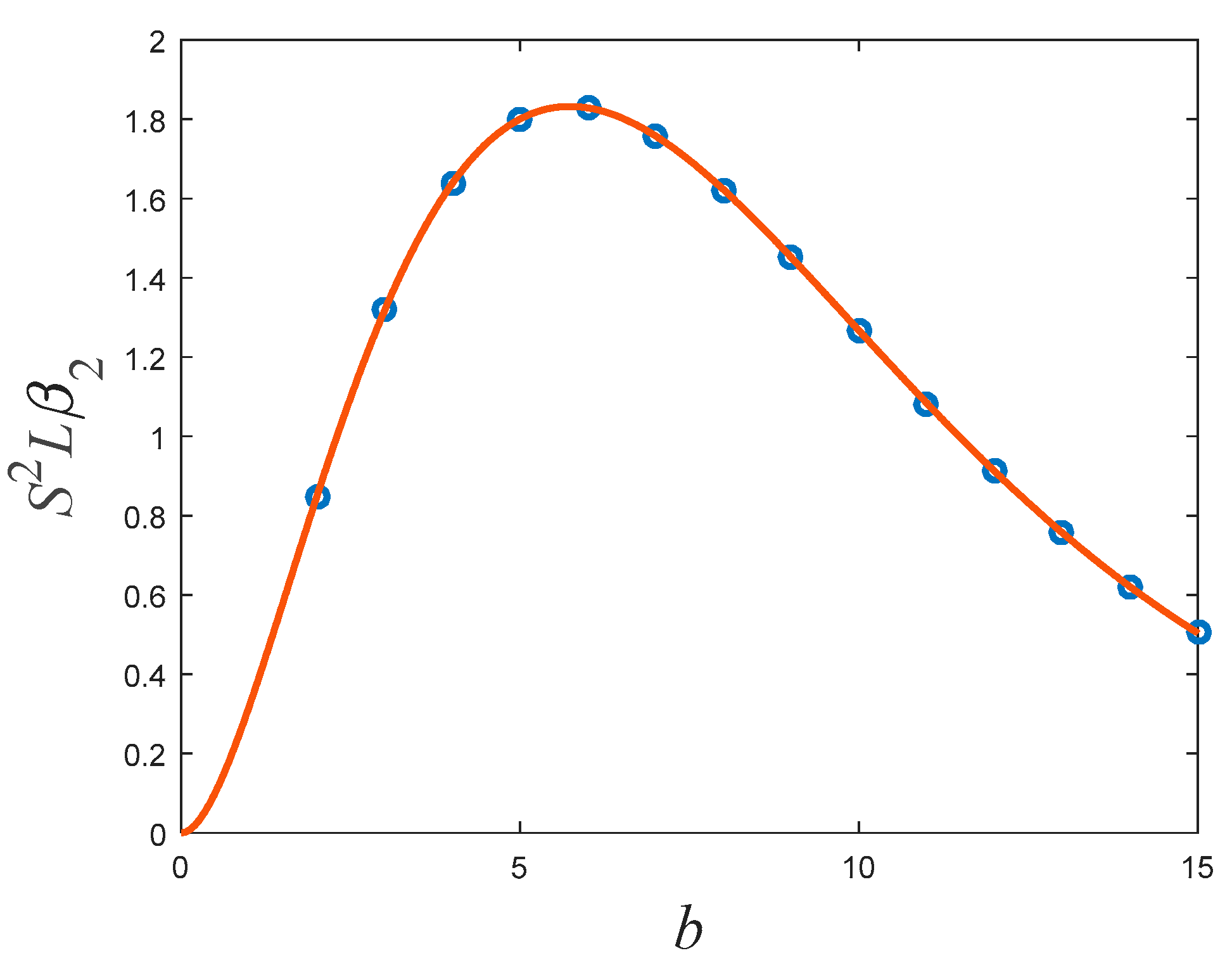
where b = log₂(N) is the number of information bits in a single symbol. Clearly, in case of the SNR < N then Equation (24) reduces to the Shannon formula $S\cong B{\log }_2\left(1+SNR\right)$. Therefore, using Equations (24) and (22), the tradeoff between the channel capacity S and the maximum distance can be written as a function of a single parameter, b:

$$S^2{L}_{\max }{\beta }_2=\frac{2}{{\pi }^2}\mathrm{acos}\left(1-2^{1-b}\right)b^2\cong \frac{4b^2}{{\pi }^2{2}^{b/2}}$$

(25)

The last approximation is valid in the large b regime. As can be seen from Figure 6, Equation (25) has a maximum of b = 6, in which case:

$$S^2{L}_{\max }{\beta }_2\cong \frac{18}{{\pi }^2}\cong 1.83$$

(26)

Obviously, these values apply only when the channel is noiseless. Therefore, they are important to evaluate the maximum errorless channel’s capacity. No better performances can be achieved without dispersion compensation (DC), regardless of the channel’s noise levels. In the presence of noise, the maximum result in Equation (26) is still valid provided log₂(SNR) > 6 (i.e., SNR > 64). Otherwise, the maximum capacity will be evaluated by substituting b = log₂(SNR) in Equation (25).

Furthermore, from the definition of G(π), it is even possible to derive an approximated evaluation of the relation between δ and Δ. From G(π) = π/4 and Equation (11), the following can be derived:

$$\frac{\pi }{4}\cong \frac{1}{2}\left[\mathrm{erfc}\left(\frac{\pi \left(1-\Delta \right)}{\delta }\right)\right]$$

(27)

and then:

$$\delta \cong \frac{\pi }{{\mathrm{erfc}}^{-1}\left(\pi /2\right)}\left(1-\Delta \right)\cong 5.6\left(\Delta -1\right)$$

(28)

In practice, this expression ignores the fact that relatively large values of Δ have a severe distortion effect on the signal, which therefore cannot be used for shorter distances, in which case a larger attenuation parameter is required, i.e., something like:

$$\delta \cong 10\left(\Delta -1\right)$$

(29)

However, Equation (28) is a very good approximation despite the many approximations and assumptions made in the derivation process.

6. Applications to Noisy Channels

In the presence of noise, the BER > 0 even for $\zeta <{\zeta }_{max}$. However, since Equation (20) is a measure of the eye opening, it can be used to calculate the channel’s BER. For a dispersion-less PAM-N channel:

$$BER\cong \frac{1}{{\log }_{2}M}\mathrm{erfc}\left(\frac{\stackrel{-}{i}}{\left(N-1\right)\sqrt{2\langle i^2\rangle }}\right)$$

(30)

where $\stackrel{-}{i}$ is the mean current and $\langle i^2\rangle$ is the current noise variance (thermic, shot-noise, RIN, etc.). Now, due to dispersion, the relative eye-opening ${\left(N-1\right)}^{-1}$ is to worsen to (20), which is when G(π) = π/4 receives a simpler form:

$$\frac{\Delta I\left(\zeta \right)}{I_0}=\frac{1}{N-1}\left[1-N{\sin }^2\left(\frac{{\pi }^2\zeta }{4}\right)\right]$$

(31)

Consequently, since after detection the current is proportional to the optical intensity, the channel’s BER can be estimated by:

$$BER\cong \frac{1}{{\log }_{2}M}\mathrm{erfc}\left(\left[1-N{\sin }^2\left(\frac{{\pi }^2\zeta }{4}\right)\right]\frac{\stackrel{-}{i}}{\left(N-1\right)\sqrt{2\langle i^2\rangle }}\right)$$

(32)

Therefore, for a given noise level and a given fixed BER, the power penalty $\eta$ (notice again that after detection the current is proportional to the optical power) is proportional to:

$$\eta \left(0,\zeta \right)=\frac{\stackrel{-}{i}\left(\zeta \right)}{\stackrel{-}{i}\left(0\right)}={\left[1-N{\sin }^2\left(\frac{{\pi }^2\zeta }{4}\right)\right]}^{-1}$$

(33)

Clearly, when $\zeta \to {\zeta }_{max}$, Equation (33) diverges. More generally, the power penalty from the distance ${\zeta }_0$ to $\zeta$ is:

$$\eta \left({\zeta }_0,\zeta \right)=\frac{\stackrel{-}{i}\left({\zeta }_2\right)}{\stackrel{-}{i}\left({\zeta }_1\right)}=\frac{1-N{\sin }^2\left({\pi }^2{\zeta }_0/4\right)}{1-N{\sin }^2\left({\pi }^2\zeta /4\right)}$$

(34)

and since the penalty is measured in dB, then for short distances it can be approximated by:

$$10{\log }_{10}\eta \left({\zeta }_0,\zeta \right)\cong \frac{10}{\ln 10}N\frac{{\pi }^4}{16}\left({\zeta }^2-{\zeta }_0^2\right)\cong 26.44N\left({\zeta }^2-{\zeta }_0^2\right)$$

(35)

In Figure 7, Equations (34) and (35) are plotted as a function of the fiber’s length z. The divergence at $\zeta \to {\zeta }_{\max }$ is clearly shown. These simple expressions can be applied for any channel regardless of its noise level.

7. BER Analysis

The maximum transmission distance Equation (22) was determined for an ideal bare system. On the one hand, it did not incorporate passive or active dispersion compensation elements (to keep the system affordable), and on the other hand, it did not take into account degrading effects, such as signal chirp, polarization effects, jitter, spectral width, nonlinear effects, and noise (to find the fundamental system’s limitations). The analysis in Section 6 did incorporate noise but used ideal filters.

In this section, we validate the analytical results of the previous sections using a real parameters simulation. We investigate the channel’s BER and its power penalty as a function of the fiber’s length and filter’s bandwidth. The consistency of these realistic results with the analytical evaluations presented in Equations (22) and (34) is investigated.

To simulate the channel using commercial software for BER analysis, we take advantage of the equivalence between the smooth rectangular spectral filter (Equation (11)) and super Gaussian (SG) filters. Specifically, the following SG spectral filter:

$$H\left(f\right)=\exp \left[-\frac{1}{2}\ln 2{\left(\frac{2f}{FWHM}\right)}^{2m}\right]$$

(36)

where FWHM is the filter’s spectral intensity full-width-at-half-maximum, and m is the SG’s order, which can replace with great accuracy the smooth rectangular filter of Equation (11) if:

$$m=\frac{\sqrt{\pi }}{\ln 2}\frac{\Delta }{\delta } \mathrm{and} FWHM=\Delta \cdot 2^{-1/2m}=\Delta \cdot 2^{-\delta \ln 2/2\Delta \sqrt{\pi }}$$

(37)

Figure 8 illustrates the similarity between the smooth rectangular filter (Equation (11)) and the SG (Equation (30)) filter, provided the parameters for Equation (31) are chosen. The figure presents high agreement between the two.

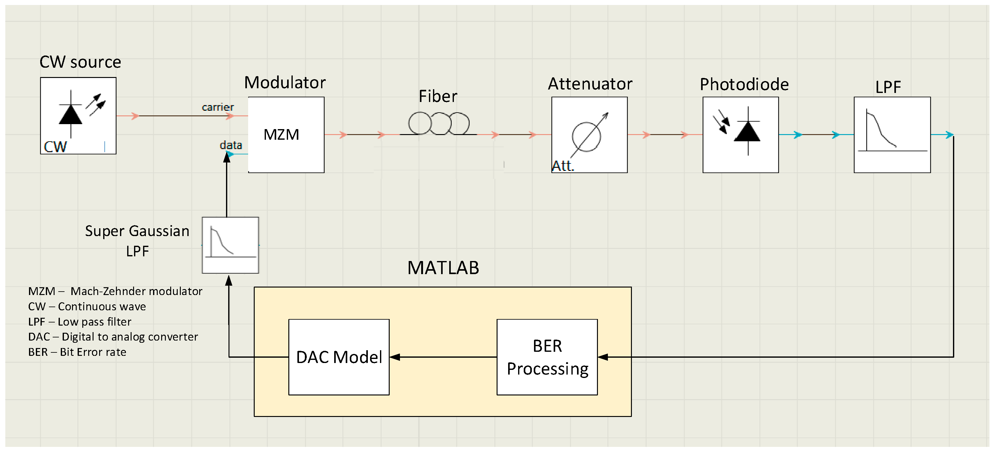
To study the BER performance of a realistic optical link, a simulation was conducted of a PAM-4 transmission using a combination of Matlab and VPI software tools over a standard single-mode fiber (ITU-T Rec. G.652). This system is presented in Figure 9. The electrical domain modulating signal of 53 Gbaud PAM-4 was generated by the digital-to-analog converter (DAC) modeled by Matlab and introduced an electrical output swing of 0.8 Vpp. This output signal was injected into the VPI simulation software, where the electrical DAC output signal passed through an SG LPF and was converted into the optical domain by a Mach–Zehnder modulator (MZM) with Vπ of 4 V. After this, the signal was transmitted over a short fiber (<4 km), converted to the electrical domain by a photodiode with referred input noise of $20p\frac{A}{\sqrt{Hz}}$, and passed through a 50 GHz (at 3 dB) LPF. The simulation’s output consisted of samples of the receiver output, which in turn were loaded back to the BER processing. The LPF in the simulation is a combination of the detectors limited bandwidth and any additional filter, electrical, or digital associated with the receiver side.

Figure 10 presents nine BER vs. optical attenuation curves for different fiber lengths (km) using a 2nd order SG filter with a 3 dB bandwidth (BW) at 40 GHz (half FWHM of the filter intensity).

It was found that the maximum fiber length that enabled a pre-FEC BER value of 1 · 10⁻³ was 3.2 km. This value was shorter than the theoretical value of 3.77 km obtained above. This mismatch was associated with some differences between the two analyses (realistic simulation vs. theoretical). First, the theoretical analysis was evaluated for a BER value of 0.5, and second, in the theoretical analysis, ideal (i.e., noiseless) detectors were considered, while in the more realistic simulation, additive (thermal) noise was introduced.

Analysis results for the attenuation penalty vs. fiber length (km) for 1st, 2nd, and 3rd order SG filters with a 3 dB BW at 40 GHz and 80 GHz are shown in Figure 11a,b, respectively. The dashed curve stands for Equation (34) (blue curve in Figure 7).

The purpose of the comparison to the wide (80GHz) filter’s performance is to emphasize the effect of the narrow one.

The penalty was evaluated at a BER of 1e-3 and plotted vs. the fiber length. Therefore, the penalty is with respect to the same system but without the fiber (which is already at a 14 dB loss).

The simulation results show that beyond 3.3 km there is a drastic decline in the BER performance. Referring to a BER value of 0.5, this result is consistent with the fundamental limit of 3.77 km (see Table 1) and with the theory of Equation (34). In the PAM-8 case presented in Figure 12, declines in the BER performance occur for distances larger than 2.3 km, which is again consistent with the fundamental limit of 2.62 km. Moreover, as can be seen from these data, a narrower spectral bandwidth is associated with a greater dependence on the SG order. This conduct is consistent with the following reasoning. Using Equation (37), the SG equivalent of Equation (28) can be written as follows:

$$m=-\frac{\ln \left[-2\frac{\ln \left(\pi /4\right)}{\ln 2}\right]}{2\ln \left(2BW/\Delta \right)}\cong \frac{0.18}{\ln \left(2BW/\Delta \right)}$$

(38)

This relation can easily be derived from the requirement H(π) = π/4, where H(π) is taken from Equation (30). This equation suggests that as the electrical filter’s bandwidth approaches half the data rate (i.e., the symbol’s rate is ~26.5 GB/s in this case), the optimal SG order increases and eventually diverges (in which case the filter has a rectangular shape). As can be seen from Figure 11 and even Figure 12, the system’s power penalty shows high agreement with the simple analytical expression Equation (34) (see the resemblance between these numerical plots and the analytical Figure 7). Moreover, the system’s BER performance improves with an increase in SG order m. As can be seen from these figures, the improvement in BER from m = 1 to m = 2 is considerably higher than the improvement from m = 2 to m = 3, and this improvement is larger when BW is 40 GHz compared to cases where it is wider (80 GHz). It is shown in Figure 13 that the best transmitted bandwidth is between 30 GHz and 40 GHz (Equation (38) predicts around 28 GHz, however, as Figure 5 shows, the maxima are very flat, and 20% changes have minor effects on the maximum distance). When the filter is wider than that, the signal becomes more susceptible to dispersion distortion, and consequently the power penalty increases.

8. Summary

The fundamental limitations that dispersion imposes upon data transport in PAM-N protocol-based channels without any dispersion compensation module (passive or active) were analyzed. It was shown analytically and using numerical simulations that the fundamental distance limit, beyond which no data decoding is feasible, can be evaluated using the expression ${\beta }_2{L}_{\max }{B}_2=\frac{2}{{\pi }^2}\mathrm{acos}\left\{\frac{N-2}{N}\right\}$. As an example, after choosing practical values for B (53 GBaud) and β₂ (ITU-T Rec. G.652), the maximum distances for PAM-4 and PAM-8 were found to be 3.7 km and 2.3 km, respectively.

Furthermore, it was shown that the product of the square of the channel’s capacity and the maximum distance was bounded by the following expression:

$S^2{L}_{\max }{\beta }_2\cong \frac{18}{{\pi }^2}\cong 1.83$, for which case the number of bits per symbol is b = 6.

In the presence of noise, for a given channel’s noise level and a given BER value, the power penalty (in dB) from a fiber’s length $z_0$ to $z$ can be approximated by the simple expression $26.44N{\beta }_2^2{B}^4\left(z^2-z_0^2\right)$.

To further validate the analytical analysis, simulations of PAM-4 and PAM-8 short-reach transmissions were introduced in Figure 10, Figure 11 and Figure 12. The simulation results showed dispersion limitations that were consistent with the fundamental dispersion limitation presented in Table 1, and the spectral bandwidth in the SG filter order behavior (Section 6) was consistent with the analytical solution derived in Equation (32). Moreover, the power penalty showed high agreement with the analytical analysis of additive noise and dispersion presented in Section 6.