Abstract
Very short-term load demand forecasters are essential for power systems’ decision makers in real-time dispatching. These tools allow traditional network operators to maintain power systems’ safety and stability and provide customers energy with high reliability. Although research has traditionally focused on developing point forecasters, these tools do not provide complete information because they do not estimate the deviation between actual and predicted values. Therefore, the aim of this paper is to develop a very short-term probabilistic prediction interval forecaster to reduce decision makers’ uncertainty by computing the predicted value’s upper and lower bounds. The proposed forecaster combines an artificial intelligence-based point forecaster with a probabilistic prediction interval algorithm. First, the point forecaster predicts energy demand in the next 15 min and then the prediction interval algorithm calculates the upper and lower bounds with the user’s chosen confidence level. To examine the reliability of proposed forecaster model and resulting interval sharpness, different error metrics, such as prediction interval coverage percentage and a skill score, are computed for 95, 90, and 85% confidence intervals. Results show that the prediction interval coverage percentage is higher than the confidence level in each analysis, which means that the proposed model is valid for practical applications.
1. Introduction
Since it was discovered in the late 1820s and early 1830s, electric power generation has become—and it will continue to be—a relevant energetic vector involved in most developed countries’ socio-economic activities [1,2]. In order to reduce the greenhouse gases associated with electricity production, some studies in the literature point out that it is necessary to decrease the energy intensity of today’s electrical-powered devices through new technological advances [3]. However, this efficiency improvement will not be enough to balance the expected growth in demand for energy in the short term [4,5]. This energy demand increase will be based on how quickly economies develop and societies’ desire for a better way of life [6] through new electrical household equipment or full or hybrid electric transport [4,7]. Moreover, both the increase in energy demand and renewable self-supply installations will increase the volatility in energy demand, making activities carried out by the current power systems’ controllers, such as real-time dispatching or stochastic unit commitment, more uncertain [8].
If reversible hydropower electric plants are not taken into account, technical limitations make the development of bulk energy storage systems impossible so, energy demand and generation had to be balanced at every moment to guarantee electric power systems’ safety and reliable operation [9,10]. No matter the power system’s size, many decisions, such as real-time dispatch, economic dispatch, or maintenance planning, are based on customer demand [11]. Therefore, to keep grids within the bounds of stability and to compute their operating schedules, power systems’ decision makers forecast their customers’ energy demand. In addition, these energy demand predictions need to be highly accurate in the short term, when there are a significant percentage of non-schedulable renewable energy sources.
A review of the literature [9,12,13] suggests that energy systems’ decision makers use scheduling algorithms that implement forecasters with different prediction horizons in order to analyze future power demand. Based on recently published studies, energy demand forecasters are categorized as follows in terms of prediction horizon:
Very Short-Term (VST): predictions computed by these forecasters are used for making real-time decisions about activities such as real-time dispatching or power smoothing [14]. Therefore, predictions are made from few seconds up to one hour ahead [15].
Short-Term (ST): values calculated through these forecasters are applied by power systems’ decision makers’ to well-known unit commitment and economic dispatch schedule activities [16]. Thus, predictions for such activities must be made from a few hours up to a day ahead [9].
Medium-Term (MT): the values produced by these forecasters are used to analyze weekly power demand fluctuations, as well as to schedule power systems’ infrastructures maintenance operations [17]. Hence, forecasters predict customers’ energy demand from days up to a few weeks ahead [12].
Long-Term (LT): these forecasters’ values are traditionally used to examine the need for new infrastructure in upcoming years in order to be able to meet customers’ power demand, as well as for power assessment [9]. Therefore, these forecasters compute a system’s power demand requirements from months up to years ahead [13].
Given the expected increase not only in energy demand but also in that demand’s volatility, as well as the desire to continue guaranteeing power supply under a system’s safety conditions, accurate VST forecasters must be developed [18]. As a consequence, this study analyzes the different VST energy demand prediction models found in the literature to develop our model.
Over the last decades, as computation techniques progressed, VST energy demand forecasters did as well, achieving more accurate predictions [19]. Depending on the type of model used to develop a forecaster, VST energy demand forecasters can be grouped into autoregressive (AR) or artificial intelligence (AI) models [15,16]. Autoregressive models are based on fixing relationships between selected parameters through the use of the chosen parameters’ time-series databases [20]. The main drawback of these models is their limited capacity to predict sudden changes in non-linear systems, as occurs in energy demand or renewable power generation. Hence, AR models must be combined with AI models in order to be able to predict energy demand with sufficient accuracy [21,22]. Most AR models are of three types: persistence models, which are commonly used as a benchmark in evaluating the results of newly developed forecasters, autoregressive moving average (ARMA), and autoregressive integrated moving average (ARIMA) forecasters.
AI models, which are also known as machine learning models, use bigger databases than AR models do. Additionally, unlike AR models, AI models are able to forecast sudden changes in non-linear systems. However, AI models require more time-series information than AR models in order to properly establish relationships between the chosen parameters [22,23], so greater computational resources are needed. Because AI models are able to predict linear and non-linear systems’ parameters with high standard of accuracy, they have been used in fields, such as renewable generation and energy demand prediction [8,15]. Although AI models are classified in several groups, most developed forecasters rely on using as baseline artificial neural network or support vector machine models [22,24].
In addition, some studies in the literature suggest that combining single approaches increases forecasting accuracy. This choice, which is known as hybridization or ensembling, is commonly applied to ST forecasters or longer prediction horizons [9,24], as it must be keep in mind that the longer the horizon, the greater the models’ error [25,26]. While some studies suggest that ensemble models should be developed for VST forecasters, other studies that have developed single approaches achieve similar results to those provided by ensemble models [27,28]. After reviewing and contrasting the results of these studies, we decided to develop a single approach AI forecaster as our model’s baseline.
Traditionally, researchers have focused on the development of prediction point forecasters (PPF), which only produce a single value for the chosen prediction horizon. Nevertheless, recent publications in literature claim that PPFs will have little accuracy improvement in the short term and that their partial information will not be enough to accurately predict volatility in future energy demand [29,30]. Therefore, some authors proposed prediction interval forecasters (PIF) as a solution to improve the quality of the provided information, making it more reliable for a grid’s decision makers’ [31,32]. Even though PIFs have been proposed recently, their suitability has been analyzed for the energy demand [32] and renewable generation prediction [30,31] research fields.
From the few studies available in literature, PIFs can be organized along two dimensions. The first dimension classifies forecasters by examining whether a PPF is applied as a baseline to calculate the interval [25,33], whereas the second dimension relates to whether researchers assume that the behavior of the parameters involved in the forecasters can be expressed through a probability density function (PDF) computed with the variables’ historical databases [34].
The first dimension splits PIFs into direct or indirect PIFs, denoted as DPIFs and IPIFs, respectively. While IPIFs are based on the use of a predicted value calculated through a PPF as a baseline for the interval’s value prediction, DPIFs predict the interval directly without the use of a PPF value. A review of the literature suggests that even though researchers are developing both DPIFs [35,36] and IPIFs [33,34,37,38,39], more effort is going into IPIF, and thus there more published studies involving IPIFs. The second dimension splits PIFs into parametric and non-parametric forecasters. With parametric forecasters, researchers assume that the parameters involved can be described by PDFs such as Gaussian or Laplacian distributions [31,38,40], whereas with non-parametric forecasters they do not make this assumption [34,35,41].
The aim of this paper is to develop an IPIF to predict energy demand 15 min ahead. The IPIF relies on the mathematical analysis of the effect of each PPF parameter in the final output and through function linearization compute the energy demand’s prediction interval. These study’s key findings are as follows:
A novel VST parametric indirect prediction interval energy demand forecaster, with a prediction horizon of the next 15 min, is proposed in order to reduce power systems’ uncertainty level. The model developed is based on combining a PPF that predicts the energy demand’s point value with mathematical concepts and a t-Student PDF that predicts the interval. Because studies in the literature propose different PPFs, the most popular models were examined to choose the most suitable one for our energy demand prediction. The root mean square error metric is calculated to compare the results provided by each programmed PPF.
Prediction interval coverage percentage (PICP) and skill score error metrics are computed for different confidence levels (95, 90, and 85%) in order to analyze the accuracy of our developed PIF, as well as the width of the predicted intervals. In addition, the final forecaster achieves higher PICP values than the stated confidence levels in all analyzed situations. Hence, as noted in the literature [33,34], when this condition is satisfied, the proposed model is acceptable for forecasting the desired parameter.
The remaining sections of this paper are organized as follows. Section 2 explains the energy demand PPF developed and the PIF methodology proposed. Section 3 presents the error metric results for the programmed PPFs and the developed PIF. The conclusions drawn from this research are summarized in Section 4.
2. Developed Methodology
As explained in the previous section, a few studies in the literature started to claim that PPFs will not be able to continue predicting energy demand with sufficient accuracy in the short term [29,30]. This statement is based on the fact that both energy demand and energy volatility will increase in the coming years [8]. Therefore, we propose the development of an energy demand PIF to address and resolve power system decision makers’ challenges in real-time dispatching.
Having conducted a literature review [33,34,37], we decided to develop a parametric IPIF. Our proposed methodology followed two main steps: we first examined different single PPFs and chose the most suitable model for VST energy demand forecasting purposes, and we then used the value given by the PPFs as a baseline in a mathematical model to calculate intervals. Because there are two well-differenced steps, Section 2.1 discusses the PPF models examined, whereas Section 2.2 presents the model proposed for interval computation. Finally, Section 2.3 shows the error metrics computed in order to analyze the programmed forecasters’ accuracy.
2.1. Analysed PPF Models
In recent years, researchers have developed many AI models not only for energy demand forecasting purposes but also for other fields, such as power prediction for renewables. For instance, some of the most frequently studied AI models are artificial neural networks (feedforward [20,42], recurrent [43,44], or wavelet [15,45]); support vector machines [46] and its support vector regression [11] variation; regression trees [47] or genetic algorithms [22]. Neural networks rely on the human brain’s mathematical replication in order to establish relationships between a system’s parameters, no matter whether the system is governed by linear or non-linear equations. With regard to support vector models, they are based on computing a set of equations, which describe system’s behavior. Regression trees or genetic algorithms apply classical logic and generalize it in their algorithms to fit a model’s parameters. Of the above algorithms, we decided to compute feedforward neural networks, recurrent neural networks and support vector machines, based on recently published results [11,15,20,22,43,46] and their ease of implementation. In addition, we decided to program a persistence model to use it as a benchmark and quantify the improvement in accuracy relative to other models’ predictions [42,45].
2.1.1. Persistence
Persistence models are based on the idea that a strong correlation exists between parameters’ actual values and the selected prediction horizon’s values. This model is described in Equation (1) as,
where is the forecasted parameter, represent the moment where the prediction is made and refers to the selected prediction horizon. Thus, by relying on strong correlation idea, the persistence model assumes that the current parameter’s value will not change between the actual moment and the chosen prediction horizon [19]. Taking into account its easy programmability and low computation cost, the persistence model is commonly used to develop VST forecasters, as well as a benchmark to compare the predicted values obtained by new forecasters and quantify the accuracy improvement [9,23,29,47,48].
2.1.2. Artificial Neural Networks (ANN)
The main advantage of ANNs is their capacity to model any system through a combination of non-linear functions, historical databases, and learning iterative algorithms [49]. In addition, ANNs’ generalization skill, i.e., their ability to produce accurate forecasts from previously unseen data, makes them suitable not only for activities such as perception, pattern recognition or regression [50,51], but also for use in many research fields such as renewable generation or energy demand forecasting [8,15,16,22,24]. A review of the literature on VST forecasters suggests that, among all possible ANNs, PPFs’ feedforward and recurrent neural networks provide accurate results [20,42,43,44] and are easy to implement.
Feedforward Neural Networks (FFNN)
With regard to FFNNs, processed information flows forward, from forecaster input to output layers. To develop this model, the following set of parameters must be analyzed: the model’s number of layers, each layer’s number of neurons, the neurons’ activation functions, and iterative training algorithm for each layer. In addition, neurons are the smallest unit of the model, and they are responsible for computing the model’s mathematical operations. The K-neuron of any ANN will be governed by the following mathematical equation,
where refers to the k-neuron’s computed value through the use of a certain set of parameters. represents each layer’s neurons’ activation user-selected functions, such as linear or sigmoid function [52], while and are each neuron’s synaptic connections and bias value (respectively), which are fitted through the iterative training algorithm. Further information concerning the neurons’ modeling and their parameters can be found in [49].
Recurrent Neural Networks (RNN)
RNNs have essentially the same set of parameters that FFNNs do, the only difference being the addition of the z−t time delay function. In contrast to FFNNs, RNNs’ information flows not only forwards but also backwards through the use of loops. Therefore, the hidden layers’ outputs are used again as inputs to the previous layers, and their z−t parameter needs to be defined. Although the application of loops increases the model’s learning skills, it has the disadvantage of increasing training time [45].
2.1.3. Support Vector Machines (SVM)
Similar to ANNs, SVM forecasters are used to model any system no matter whether it is governed by linear or non-linear equations. In this study, the SVMs’ regression skill is used to fit vector coefficients through the use of historical databases. Just as ANNs’ use neurons to produce their predictions, SVMs use their vectors to forecast future values. Although SVMs and ANNs share similarities due to the fact that both optimize their parameters through regression algorithms, SVM models have the advantage of being able to change all of a model’s parameters if a better configuration is found during the training step. However, ANNs are not able to calculate these variations and they maintain their parameters throughout the whole training step [51].
To perform a regression activity, SVMs use different kinds of transformations, which are denoted as kernel functions. These kernel functions modify a model’s vectors’ coefficient values through an iterative process, until the point where the difference between the actual and forecasted value reduces to a residual error chosen by the user. In addition, the main advantage of kernel functions arises from the fact that no matter how complicated the real system is, kernel functions will be able to converge on the optimal solution without getting stuck in a local minima [53].
2.2. Proposed IPIF Model
Let us suppose any electric power system’s energy demand (), no matter its size, can be expressed through the combination of an unknown function () and a set of input parameters (), as in Equation (3),
Because it is difficult to obtain the energy demand’s analytical expression (), the purpose is to use the most accurate PPF presented in the previous section, so an approximation of the real system can be analyzed. Therefore, the system’s energy demand approach is mathematically expressed as,
where refers to the deviation between the actual value and the IPIF’s predicted value and represent the PPF’s set of real system parameters, which will be optimized during the training step . Thus, the PPF model is described as,
By combining Equations (4) and (5), as well as Taylor’s first-order polynomial approximation, deviation can be expressed in terms of,
where is the gradient of the PPF’s function and can be described as,
where L is the number of parameters. In addition, Equation (6) can we reordered as follows,
As we developed a parametric IPIF, the following assumptions are made: in our statistical analysis, and behave as random variables and deviation also behaves as a random variable described through a Normal distribution and is independent from . Therefore, Equation (8) can be expressed in root mean square error terms as,
where denotes the expectation, that can also be mathematically expressed as,
is the Jacobian matrix where condition must be fulfilled. While is the number of parameters, is a set of the training database used to fit PPF model. Combining Equations (9) and (10) yields,
where is the unbiased estimator of and its value is computed as,
It must be kept in mind that the estimator only can be properly calculated if the condition is satisfied. Finally, for a sufficient number of F samples taken from the training database, random parameter can be calculated as,
In addition, the parameter can be approximated by a t-Student distribution with of degrees of freedom [54]. The proposed IPIF will use the following equation to compute the intervals for a chosen confidence level of ,
where refers to the error rate chosen by the user, and represents the probability value obtained through the t-Student’s distribution for a chosen error rate and degrees of freedom. As can be concluded from Equation (14), the more accurate the PPF is , the more reliable the IPIF’s interval will be.
2.3. Computed Error Metrics
Because we suggest the development of an IPIF whose intervals are computed using as baseline a PPF’s predictions, both forecasters’ error metrics must be examined. While PPF’s error metrics are used to select the most suitable of above explained models, IPIF’s error metrics analyze not only forecasters’ reliability but also predicted intervals sharpness.
2.3.1. PPF Error Metrics
A review of the literature [4,6,10,18,26,39,46] suggests that the root mean square error (RMSE) and R-squared (R2) error metrics are commonly calculated not only to analyze the PPFs’ prediction accuracy, but also to compare them against other studies’ results. Therefore, in this study both error metrics are calculated through the following equations,
where represent the number of predicted values during a time lapse, refers to the actual parameter’s value for sample, is the PPF’s predicted value for sample , and is predictions’ averaged value. Due to the database resolution, 15 min, the number of predicted values during a day is,
2.3.2. PIF Error Metrics
From previous published studies [30,31,33,37,39], it is known that the PIF’s error metrics fall into two categories: reliability or sharpness indexes. Reliability error metrics, such as prediction interval coverage percentage (PICP), examines how many of the actual values fall into the predicted intervals, whereas the sharpness error metrics such as skill score (SS) analyze the predicted intervals’ width. In this study, we calculated four error metrics, a couple of each category.
Before describing the computed error metrics, it is necessary to define the concept of prediction interval bound (PIB), which is composed of the upper (UB) and lower bounds (LB). Therefore, the PIB for a chosen error rate α and sample is mathematically defined as pair. From Equation (14), , and are expressed as below,
The most commonly computed and best-known PIF error metric is the PICP index. For a given set of samples with their respective PIBs, the PICP index analyzes and calculates as a percentage the number of samples that fall into their respective PIBs. This index is mathematically expressed as,
In addition, as is supported by literature [55,56], a proposed model is considered acceptable when the obtained is equal to or greater than the confidence level (CL) chosen by the user . Therefore, the higher the , the better the model’s reliability. Moreover, if this condition is not fulfilled, the proposed model must be reanalyzed until this condition is met. Once the required condition is met, other error metrics can be computed, such as the coverage error (CE), whose value is computed through
Based on the fact that , must always be at least equal to or greater than zero. The higher the , the better model’s reliability. Moreover, as noted in the literature, it is also necessary to examine the sharpness of the predicted intervals [33,56], i.e., the interval width. In order to understand the computed sharpness error metrics, it is necessary to define the mathematical concept prediction interval width (PIW), for a random sample and chosen error rate:
With regard to the interval sharpness error metrics, a skill score (SS) was computed to quantify predicted interval width for a set of N samples. SS is mathematically expressed as,
must always be positive, and the closer this value is to zero, the narrower the computed intervals are. Often is normalized by parameter P in order to facilitate comparison with other studies. P’s order of magnitude is related to the forecasted variable.
While the index takes into account whether an actual value falls into in its computation algorithm, the normalized prediction interval averaged width (NPIAW) just takes into account a set of intervals for a certain error rate, whose values are averaged and normalized as described below,
3. Results and Discussion
A historical database of energy demand from a private company was used to examine the accuracy of the algorithms explained above. All models in the present study were trained with the energy demand database for the whole of 2017 for 15 min resolution, whereas the whole database for 2018 with same resolution was used for the validation analysis. Thus, each database has a length of 35040 samples. In addition, the input vector used to develop the FFNN, RNN, and SVM models was made up of: season, the time of day the prediction was made, and energy demand values during the last 24 h with 15 min resolution. Both the proposed energy demand IPIF and all of the PPFs presented below were programmed in MATLAB®.
3.1. PPF Model’s Results
This section shows the error metric results obtained through the PPFs described in Section 2.1. The most accurate model is the one that was chosen in order to use its predictions as the baseline in developing our IPIF. In addition, the PPF error metrics were compared against the error metrics given in other studies in the literature.
3.1.1. Persistence Model
Based on the deviation between actual and predicted energy demand values, Table 1 shows the RMSE and R2 indexes for the training and validation steps.

Table 1.
Computed RMSE and R2 indexes’ values for the persistence model.
Moreover, these indexes’ values were used as the baseline benchmark for quantifying the accuracy improvement obtained by other programmed PPF models’ by using Equation (25),
where is always an error metric computed through the persistence model and is the error metric computed through the model whose improvement needs to be quantified.
3.1.2. FFNN Model
As explained in Section 2.1.2, when a FFNN forecaster is developed, the following set of parameters must be fit: the model’s number of layers, each layer’s number of neurons, each layer’s neurons’ activation functions and iterative training algorithm (see Figure 1). With regard to the training step’s algorithms, a review of literature [15,45,53] agreed on the Levenberg–Marquardt (LM) algorithm being the most suitable choice for developing their forecasters, so the LM training algorithm was used in this study based on those previous studies’ accurate results. Moreover, Panchal et al. [57] concluded through the development of several ANN structures that two hidden layers structures do not necessarily improve forecasters’ accuracy and increases the possibility of getting stuck in a local minima, so a single hidden layer PPF structure was developed in our study. Although there are different activation functions that can be chosen for the neurons in each layer of the forecaster [52], in this forecaster, we chose the configuration usually suggested in the literature: a logarithmic sigmoid transfer function in the hidden layer and a linear transfer function in the output layer [42,43,44,45]. Therefore, the last parameter that needed to be select was the hidden layer’s number of neurons.
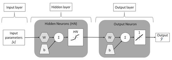
Figure 1.
FFNN forecaster’s layout.
Related literature shows that the only available methodology for fixing the number of neurons in each layer relies on a sensitivity analysis [42,43,44,45]. In addition, the use of MATLAB® and its random initialization in the training step increases the risk of non-convergence. Therefore, to reduce this risk, each analyzed structure was repeated five times and the results from the training and validation steps were averaged. To fix the FFNN’s hidden layer’s number of neurons, the RMSE index was computed; then, the R2 index was calculated for the best structure. Table 2 shows the averaged results for the FFNN structures analyzed.
Table 2.
FFNNs structures’ averaged results for fixing hidden layer’s number of neurons.
The results in Table 2 suggest that there is little variation between analyzed structures’ results when the hidden layer’s neurons were modified. Based on the fact that forecasters with lower RMSEs are more accurate, the 10-neuron structure was the most accurate structure for the training database, whereas the 15-neuron structure was the best with the validation database. Taking into account that our goal was to maximize the forecaster’s generalization capacity, i.e., obtain the most accurate predictions through previously unseen values, we chose to compare the 15-neuron structure against the results from the other PPFs. Table 3 summarizes 15-neuron configuration’s error metrics and their improvement in percentage against the benchmark model.
Table 3.
Computed RMSE and R2 index values for 15-neuron FFNN model.
3.1.3. RNN Model
Regarding the RNN model, the FFNN’s set of parameters, as well as its delay parameter, must be fit. Therefore, the training algorithm, number of hidden layers and each layer’s neurons activation functions remained the same as in the FFNN’s model. As occurred for the FFNN forecaster, the literature does not provide an analytical method for choosing the hidden layer’s number of neurons or the RNN’s characteristic delay parameter, so both parameters had to be chosen through sensitivity analyses (see Figure 2).
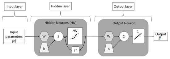
Figure 2.
RNN forecaster’s layout.
Because we had to select two parameters, we first modified the delay while holding the number of neurons constant, and then having chosen the delay, we modified the number of neurons. In this study, the procedure explained in [45] was used, where the delay was varied from 1:2 to 1:6 while the number of neurons was held at 10. After the best delay was obtained, it was held constant while the number of neurons was modified from 5 to 15, in steps of 5 neurons. The same procedure applied in the FFNN sensitivity analyses for avoiding non-convergence risk was used for the RNN forecaster. Thus, each configuration’s five tests were run and their training and validation results were averaged (see Table 4).
Table 4.
RNNs analyzed structures’ averaged results for fixing hidden layer’s number of neurons.
The results in Table 4 indicate that the first structure analyzed, where the delay was 1:2 and 10 neurons were in the hidden layer, produced more accurate predictions for both databases. Therefore, this structure was chosen in order to compare it against the other PPFs results, and Table 5 summarizes this configuration’s error metrics, as well as their improvement as a percentage against the benchmark model.
Table 5.
Computed RMSE and R2 index values for optimal RNN model.
3.1.4. SVM Model
With regard to SVM models, a couple of parameters, denoted as solvers and kernel functions, must be selected. Because there are different types of solvers and kernel functions, different combinations were analyzed in order to select the optimal configuration. These solvers serve the same function in SVM models as LM algorithms do in FFNN and RNN structures, so to avoid the no-convergence issue, five tests of each configuration were run and their results were averaged. Table 6 show the computed averaged RMSE index values.
Table 6.
Analyzed SVM structures’ averaged results for fixing solver and kernel function parameters.
The results presented in Table 6 demonstrate that there is not a single structure which minimizes both databases’ RMSE index results. Based on the fact that the PPF model needs to have higher accuracy with previously unseen data, the ‘SMO’ solver and the ‘linear’ kernel function were chosen to compare this model against the other computed models. Table 7 show the best configuration’s error metrics as well as its improvement in percentage against the benchmark model.
Table 7.
Computed RMSE and R2 index values for optimal SVM model.
3.1.5. Discussion of PPF Model
To more easily compare the results obtained by each computed PPF model, Table 8 summarizes each model’s obtained error metrics and the improvement in percentage when the results are compared against the persistence model (benchmark). For each model shown in Table 8, the value outside the brackets is the result obtained for each error metric, whereas the value inside the brackets, expressed in percentage, refers to the improvement when the values are compared against persistence benchmark. For this reason, the persistence model does not have any value inside the brackets.
Table 8.
Computed RMSE and R2 index values for each model’s optimal architecture.
Based on the results shown in Table 8, and taking into account its easier implementation and lower computational cost not only for the training step but also in producing forecasting values, the 15-neuron FFNN structure was selected. The predictions produced by this forecaster were then used as the baseline in the proposed IPIF. If FFNN results are compared against other PIF studies in the literature, a slight improvement is obtained by the developed energy demand forecaster. For instance, Zhang et al. [58] developed a VST energy demand IPIF whose FFNN forecaster’s parameters were completely different to the parameters chosen in this study. In terms of R2 index, Zhang obtained a regression value of 0.91, whereas the value obtained through this study was 0.99, demonstrating that the point forecaster slightly improves Zhang’s PPF.
3.2. IPIF Model’s Results
Based on the results in Section 3.1.5, the 15-neuron FFNN model was used as a baseline to develop our proposed IPIF described in Section 2.2. The total number of parameters in the chosen FFNN was computed as , where is the number of neurons in the hidden layer and refers to the system’s number of inputs, i.e., 15 neurons and 98 inputs, respectively. Therefore, , which represents a set of the training database used to fit the PPF model, is the last parameter to be defined in the proposed IPIF model. Thus, parameter must satisfy the following condition , where 35040 is the length of the database used to fit the PPF model and 1501 is the total number of parameters. In addition, it must be reminded that for each set, parameters present in Equations (12)–(14) must be recomputed. To be able to select the parameter that maximizes the IPIF’s accuracy, a sensitivity analysis was performed, in which several sets were examined for different error rates. Table 9 shows the results for each computed scenario on randomly chosen days. Remember that the condition must be fulfilled in order for the proposed IPIF model to be considered valid and represents the number of predicted values during each day.
Table 9.
results for computed scenarios .
From the results shown in Table 9, it can be concluded, for bigger values, that when the error rate increases the IPIF’s accuracy value decreases (see Table 9 columns or ). However, this relationship has a weaker effect or completely disappears when lower values are chosen (see Table 9 columns or ). In addition, all the analyzed scenarios presented in Table 9 satisfy the requirement, so all sets can continue being examined.
The next step was based on analyzing each scenario’s sharpness error metrics; for this purpose, the parameter was calculated for the scenarios from the previous table (see Table 10). To compute the error metric, takes the training database’s average value, 3546 kW.
Table 10.
results for computed scenarios .
Based on the results presented in Table 10, it can be concluded that, considering the same α error rate, the lower F value is the bigger the error metric is. This means that the interval width increases as the F value decreases. However, if the F value holds constant and the α error rate changes, then the bigger the α error rate is, the narrower the predicted interval is. Moreover, if the results in Table 9 and Table 10 are examined, the wider the interval, the better the accuracy. Nevertheless, this IPIF is meant to decrease the uncertainty of the energy demand in order to help power systems’ decision makers, so the user’s knowledge must be used to balance the proposed forecaster’s interval width and the model’s accuracy.
Even though the IPIF for satisfies the condition for all analyzed error rates, we realized that the values are far from the 95% accuracy level for those error metrics which are not (see Table 9). Therefore, through balancing accuracy and interval width, the most suitable combinations were selected. Table 11 shows the selected parameter for each error rate as well as the corresponding error metrics not only for the sample days shown in Table 5 and Table 10 but also for a few others, which were randomly chosen.
Table 11.
Computed error metrics for the examined scenarios
The results presented in Table 11 demonstrate that, with our forecaster and a sensitivity analysis for the parameter, it is possible to obtain IPIFs whose accuracy is close to the stated goal of 95% in terms of the analyzed error rates maintaining interval width. If we focus on the column, it can be seen that the bigger the error rate is, the bigger the value is. This fact does not rely on the predicted interval width; if Equation (22) is examined, it can be seen how is taken into account in computing values, so the higher , the higher . Figure 3, Figure 4 and Figure 5 show the predicted intervals obtained for 8 February 2018 for each examined scenario in Table 11.
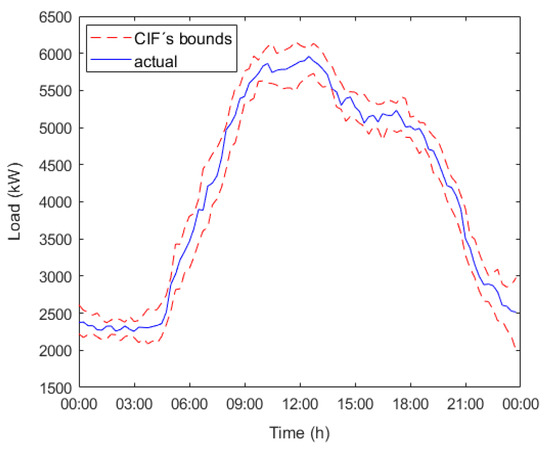
Figure 3.
Predicted intervals and actual energy demand evolution for 8 February 2018 scenario , .
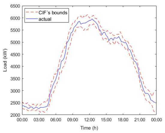
Figure 4.
Predicted intervals and actual energy demand evolution for 8 February 2018 scenario , .
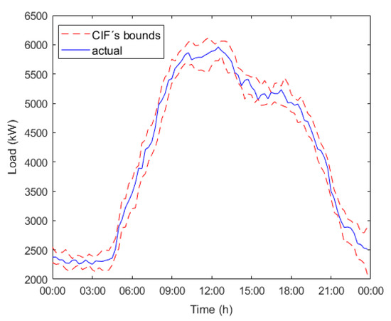
Figure 5.
Predicted intervals and actual energy demand evolution for 8 February 2018 scenario , .
Figure 2, Figure 3 and Figure 4 demonstrated that even though the error rate increases, our forecaster, with the parameter’s proper sensitivity analysis, is able to maintain high accuracy, which is close to the stated goal of 95%.
In contrast to other studies in the literature, such as Ni et al. [56] or Xu et al. [59], where error rate is fixed during the training step and PIF only predicts intervals for the chosen error rate, our model does not have this limitation. However, there are other authors in literature, such as Zhang et al. [58], who have proposed an IPIF whose error rate can be modified for similar energy demand and prediction horizon boundary conditions. Zhang et al. only provide reliability error metrics such as and in their study; Table 12 summarizes Zhang et al.’s results and our results (averaged from Table 9 )) for those reliability indexes.
Table 12.
Comparison of computed error metrics’ comparison for our proposed IPIF and Zhang et al.’s IPIF.
From the results in Table 12, we can conclude that for similar prediction horizon conditions (Zhang et al. forecaster’s makes predictions 10 min ahead, whereas in this study the forecaster makes predictions 15 min ahead), similar relative energy demand evolution along days (Zhang et al. energy demand varies in a range from 1500 to 3000 kW, whereas in this study it varies from 2500 to 6000 kW) and similar input parameters (Zhang et al. forecaster’s uses Month, Day, Hour, Minute, Day Type, Outdoor air temperature, Outdoor air relative humidity and previous load values as input parameters, in this study the forecaster uses season, time of day and previous load values) our forecaster is a slightly improvement over the IPIF proposed by Zhang et al. [58]. The main difference between both forecasters relies on the input parameters selection; Zhang et al. introduced meteorological parameters as input parameters, whereas in this study they are discarded based on the results obtained in a previous study [60]. The results of [60] demonstrated that the introduction of meteorological parameters reduces the accuracy of final forecaster for chosen prediction horizon.
4. Conclusions
The goal of this study was to develop an energy demand parametric IPIF. Our proposed forecaster predicts energy demand intervals for a 15-min-ahead time horizon and using an α error rate chosen by the user. The model and its error metrics were computed through a private company’s energy demand historical database. The main findings from this study are:
- (1)
- A novel VST parametric IPIF was proposed in order to predict energy demand intervals 15 min ahead. Our forecaster relies on the combination of a PPF to predict energy demand point values, and mathematical concepts as well as t-Student PDF to predict the interval. Concerning the analyzed PPFs, the FFNN model arose as the most suitable one, due to the fact that it has the lowest training and validation RMSE indexes, 0.0853 MW and 0.0766 MW, respectively.
- (2)
- The developed IPIF’s accuracy was examined for different error rates, namely 0.05, 0.10, and 0.15. After performing several analyses, it was concluded that higher error rates generate a decrease in the model’s accuracy. However, in our model, this disadvantage can be limited if a sensitivity analysis is done for the parameter. In addition, there is a strong relationship between the forecaster’s accuracy and prediction interval width, so the knowledge that power systems’ decision makers have will allow them to choose if they prefer more accurate or narrower intervals.
- (3)
- All of this study’s numerical results have been calculated from a private company’s energy demand historical database. While the training database contains information about the company’s energy demand for 2017, the validation database contains information about the company’s 2018 energy demand. A comparison of similar studies in the literature shows that there is a slight improvement when the computed error metrics are examined. The main disadvantage of our proposed model is the fact that at least an entire year’s energy demand database was needed to develop the PPF which provides the prediction value. With regard to the proposed interval prediction mathematical model, the main advantage is that even though the model has been fitted for a chosen error rate, the user is allowed to compute intervals not only for that error rate but also for others. In addition, this study’s IPIF model is completely developed through mathematical concepts and t-Student PDF, so our suggested methodology can be applied in other fields where there is desire to predict intervals.
Author Contributions
Conceptualization, F.R. and J.M.G.; Formal analysis, A.G.; Investigation, F.R. and N.B.; Methodology, F.R. and N.B.; Resources, F.R. and A.G.; Software, F.R. and N.B.; Supervision, A.G.; Validation, F.R.; Visualization, J.M.G.; Writing—original draft, F.R.; Writing—review & editing, J.M.G. and A.G. All authors have read and agreed to the published version of the manuscript.
Funding
This research was funded by the Basque Government’s Department of Education for financial support through the Researcher Formation Program; grant number PRE_2019_2_0035. This research was funded by Fundación Caja Navarra, Obra Social La Caixa and University of Navarra for financial support through the Mobility Research Formation Program; grant number MOVIL-2019-25. This research was funded by the European Union’s Horizon 2020 research and innovation program under grant agreement No 847054. The authors are grateful for the support and contributions from other members of the AmBIENCe project consortium, from VITO (Belgium), ENEA (Italy), TEKNIKER (Spain), INESC TEC (Portugal), ENERGINVEST (Belgium), EDP CNET (Portugal), and BPIE (Belgium). Further information can be found on the project website (http://ambience-project.eu/, accessed on 27 May 2020). This research was funded by the ELKARTEK program (CODISAVA KK-2020/00044) of the Basque Government. J.M.G. was supported by VILLUM FONDEN under the VILLUM Investigator Grant (no. 25920): Center for Research on Microgrids (CROM); www.crom.et.aau.dk.
Institutional Review Board Statement
Not applicable.
Informed Consent Statement
Not applicable.
Data Availability Statement
Data sharing is not applicable to this article. Data was obtained from a private company and are not available.
Conflicts of Interest
The authors declare that they have no known competing financial interests or personal relationships that could have appeared to influence the work reported in this paper.
Disclaimer
Neither the European Commission nor any person acting on behalf of the European Commission is responsible for the use which might be made of the following information. The views expressed in this publication are the sole responsibility of the authors and do not necessarily reflect the views of the European Commission.
References
- Alarenan, S.; Gasim, A.A.; Hunt, L.C. Modelling industrial energy demand in Saudi Arabia. Energy Econ. 2020, 85, 104554. [Google Scholar] [CrossRef]
- Liu, J.; Niu, D.; Song, X. The energy supply and demand pattern of China: A review of evolution and sustainable development. Renew. Sustain. Energy Rev. 2013, 25, 220–228. [Google Scholar] [CrossRef]
- Goldemberg, J. The evolution of the energy and carbon intensities of developing countries. Energy Policy 2020, 137, 1060. [Google Scholar] [CrossRef]
- Ayvazoğluyüksel, Ö.; Filik, Ü.B. Estimation methods of global solar irradiation, cell temperature and solar power forecasting: A review and a case study in Eskişehir. Renew. Sustain. Energy Rev. 2018, 91, 639–653. [Google Scholar] [CrossRef]
- Teklu, T.W. Should Ethiopia and least developed countries exit from the Paris climate accord?—Geopolitical, development, and energy policy perspectives. Energy Policy 2018, 120, 402–417. [Google Scholar] [CrossRef]
- He, F.; Zhou, J.; Mo, L.; Feng, K.; Liu, G.; He, Z. Day-ahead short-term load probability density forecasting method with a decomposition-based quantile regression forest. Appl. Energy 2020, 262, 114369. [Google Scholar] [CrossRef]
- Afroz, Z.; Urmee, T.; Shafiullah, G.M.; Higgins, G. Real-time prediction model for indoor temperature in a commercial building. Appl. Energy 2018, 231, 29–53. [Google Scholar] [CrossRef]
- Yang, Y.; Hong, W.; Li, S. Deep ensemble learning based probabilistic load forecasting in smart grids. Energy 2019, 189, 116324. [Google Scholar] [CrossRef]
- Ahmad, T.; Chen, H. Utility companies strategy for short-term energy demand forecasting using machine learning based models. Sustain. Cities Soc. 2018, 39, 401–417. [Google Scholar] [CrossRef]
- Li, C. Designing a short-term load forecasting model in the urban smart grid system. Appl. Energy 2020, 266, 114850. [Google Scholar] [CrossRef]
- Che, J.; Wang, J. Short-term load forecasting using a kernel-based support vector regression combination model. Appl. Energy 2014, 132, 602–609. [Google Scholar] [CrossRef]
- İlseven, E.; Göl, M. Medium-term electricity demand forecasting based on MARS. In Proceedings of the 2017 IEEE PES Innovative Smart Grid Technologies Conference Europe (ISGT-Europe), Torino, Italy, 26–29 September 2017. [Google Scholar] [CrossRef]
- Carvallo, J.P.; Larsen, P.H.; Sanstad, A.H.; Goldman, C. Long term load forecasting accuracy in electric utility integrated resource planning. Energy Policy 2018, 119, 410–422. [Google Scholar] [CrossRef]
- Wang, F.; Zhen, Z.; Liu, C.; Mi, Z.; Hodge, B.M.; Shafie-khah, M.; Catalão, J.P.S. Image phase shift invariance based cloud motion displacement vector calculation method for ultra-short-term solar PV power forecasting. Energy Convers. Manag. 2018, 157, 123–135. [Google Scholar] [CrossRef]
- Rana, M.; Koprinska, I. Forecasting electricity load with advanced wavelet neural networks. Neurocomputing 2016, 182, 118–132. [Google Scholar] [CrossRef]
- Jiang, J.; Li, G.; Bie, Z.; Xu, H. Short-term load forecasting based on higher order partial least squares (HOPLS). In Proceedings of the 2017 IEEE Electrical Power and Energy Conference (EPEC), Saskatoon, SK, Canada, 22–25 October 2017. [Google Scholar] [CrossRef]
- Dudek, G.; Pelka, P. Medium-term electric energy demand forecasting using Nadaraya-Watson estimator. In Proceedings of the 18th International Scientific Conference on Electric Power Engineering (EPE), Kouty nad Desnou, Czech Republic, 17–19 May 2017. [Google Scholar] [CrossRef]
- Elsinga, B.; van Sark, W.G.J.H.M. Short-term peer to peer solar forecasting in a network of photovoltaic systems. Appl. Energy 2017, 206, 1464–1483. [Google Scholar] [CrossRef]
- Raza, M.Q.; Khosravi, A. A review on artificial intelligence based load demand forecasting techniques for smart grid and buildings. Renew. Sustain. Energy Rev. 2015, 50, 1352–1372. [Google Scholar] [CrossRef]
- Kuster, C.; Rezgui, Y.; Mourshed, M. Electrical load forecasting models: A critical systematic review. Sustain. Cities Soc. 2017, 35, 257–270. [Google Scholar] [CrossRef]
- Kuswaha, V.; Pindoriya, N.M. A SARIMA-RVFL hybrid model assisted by wavelet decomposition for very short-term solar PV power generation forecast. Renew. Energy 2019, 140, 124–139. [Google Scholar] [CrossRef]
- Prado, F.; Minutolo, M.C.; Kristjanpoller, W. Forecasting based on an ensemble Autoregressive Moving Average—Adaptive neuro—Fuzzy inference system—Neural network—Genetic Algorithm Framework. Energy 2020, 197, 117159. [Google Scholar] [CrossRef]
- Singh, A.S.N.; Mohapatra, A. Repeated wavelet transform based ARIMA model for very short-term wind speed forecasting. Renew. Energy 2019, 136, 758–768. [Google Scholar] [CrossRef]
- Li, P.; Zhou, K.; Lu, X.; Yang, S. A hybrid deep learning model for short-term PV power forecasting. Appl. Energy 2020, 259, 114216. [Google Scholar] [CrossRef]
- Shing, P.; Dwivedi, P.; Kant, V. A hybrid method based on neural network and improved environmental adaptation method using Controlled Gaussian Mutation with real parameter for short-term load forecasting. Energy 2019, 174, 460–477. [Google Scholar] [CrossRef]
- Monteiro, C.; Santos, T.; Fernandez-Jimenez, L.A.; Ramirez-Rosado, I.J.; Terreros-Olarte, M.S. Short-term power forecasting model for photovoltaic plants based on historical similarity. Energies 2013, 6, 2624–2643. [Google Scholar] [CrossRef]
- Da Silva, I.N.; de Andrade, L.C.M. Efficient Neurofuzzy Model to Very Short-Term Load Forecasting. IEEE Lat. Am. Transac. 2016, 14, 721–728. [Google Scholar] [CrossRef]
- Staats, J.; Bruce-Boye, C.; Weirch, T.; Watts, D. Markov Chain based Very Short-Term Load forecasting realizing Conditional Expectation. In Proceedings of the International ETG Congress 2017, Bonn, Germany, 28–29 November 2017. [Google Scholar]
- David, M.; Luis, M.A.; Lauret, P. Comparison of intraday probabilistic forecasting of solar irradiance using only endogenous data. Int. J. Forecast. 2018, 34, 529–547. [Google Scholar] [CrossRef]
- Li, K.; Wang, R.; Lei, H.; Zhang, T.; Liu, Y.; Zheng, X. Interval prediction of solar power using an Improved Bootstrap method. Sol. Energy 2018, 159, 97–112. [Google Scholar] [CrossRef]
- Sun, M.; Feng, C.; Zhang, J. Multi-distribution ensemble probabilistic wind power forecasting. Renew. Energy 2020, 148, 135–149. [Google Scholar] [CrossRef]
- Yan, X.; Abbes, D.; Francois, B. Uncertainty analysis for day ahead power reserve quantification in an urban microgrid including PV generators. Renew. Energy 2017, 106, 288–297. [Google Scholar] [CrossRef]
- Zhang, J.; Yan, J.; Infield, D.; Liu, Y.; Lien, F.S. Short-term forecasting and uncertainty analysis of wind turbine power based on long-term memory network and Gaussian mixture model. Appl. Energy 2019, 241, 229–244. [Google Scholar] [CrossRef]
- Liu, L.; Zhao, Y.; Chang, D.; Xie, J.; Ma, Z.; Sun, Q.; Yin, H. Prediction of short-term PV power output and uncertainty analysis. Appl. Energy 2018, 228, 700–711. [Google Scholar] [CrossRef]
- Liu, Y.; Qin, H.; Zhang, Z.; Pei, S.; Jiang, Z.; Feng, Z.; Zhou, J. Probabilistic spatiotemporal wind speed forecasting based on a variational Bayesian deep learning model. Appl. Energy 2020, 260, 114259. [Google Scholar] [CrossRef]
- Cheng, W.Y.Y.; Liu, Y.; Bourgeois, A.J.; Wu, Y.; Haupt, S.E. Short-term wind forecast of a data assimilation/weather+ forecasting system with wind turbine anemometer measurement assimilation. Renew. Energy 2017, 107, 340–351. [Google Scholar] [CrossRef]
- Verbois, H.; Rusydi, A.; Thiery, A. Probabilistic forecasting of day-ahead solar irradiance using quantile gradient boosting. Sol. Energy 2018, 173, 313–327. [Google Scholar] [CrossRef]
- Wan, C.; Lin, J.; Song, Y.; Xu, Z.; Yang, G. Probabilistic forecasting of photovoltaic generation: An efficient statistical approach. IEEE Trans. Power Syst. 2017, 32, 2741–2742. [Google Scholar] [CrossRef]
- Wang, H.; Yi, H.; Peng, J.; Wang, G.; Liu, Y.; Jiang, H.; Liu, W. Deterministic and probabilistic forecasting of photovoltaic power based on deep convolutional neural network. Energy Conv. Manag. 2017, 153, 409–422. [Google Scholar] [CrossRef]
- Junior, J.G.D.S.F.; Oozeki, T.; Ohtake, H.; Takashima, T.; Ogimoto, K. On the Use of Maximum Likelihood and Input Data Similarity to Obtain Prediction Intervals for Forecasts of Photovoltaic Power Generation. J. Electr. Eng. Technol. 2015, 10, 1342–1348. [Google Scholar] [CrossRef]
- El-Baz, W.; Tzscheutschler, P.; Wagner, U. Day-ahead probabilistic PV generation forecast for buildings energy management systems. Sol. Energy 2018, 171, 478–490. [Google Scholar] [CrossRef]
- Gutierrez-Corea, F.V.; Manso-Callejo, M.A.; Moreno-Regidor, M.P.; Manrique-Sancho, M.T. Forecasting short-term solar irradiance based on artificial neural networks and data from neighbouring meteorological stations. Sol. Energy 2016, 134, 119–131. [Google Scholar] [CrossRef]
- Ruiz, L.G.B.; Rueda, R.; Cuéllar, M.P.; Pegalajar, M.C. Energy consumption forecasting based on Elman neural networks with evolutive optimization. Expert Syst. Appl. 2018, 92, 380–389. [Google Scholar] [CrossRef]
- Koschwitz, D.; Frisch, J.; van Treeck, C. Data-driven heating and cooling load predictions for non-residential buildings based on support vector machine regression and NARX Recurrent Neural Network: A comparative study on district scale. Energy 2018, 165, 134–142. [Google Scholar] [CrossRef]
- Rodríguez, F.; Florez-Tapia, A.M.; Galarza, A.; Fontán, L. Very short-term wind power density forecasting through artificial neural networks for microgrid control. Renew. Energy 2020, 145, 1517–1527. [Google Scholar] [CrossRef]
- Jiang, P.; Li, R.; Liu, N.; Gao, Y. A novel composite electricity demand forecasting framework by data processing and optimized support vector machine. Appl. Energy 2020, 260, 114243. [Google Scholar] [CrossRef]
- Lusis, P.; Khalilpour, K.R.; Andrew, L.; Liebman, A. Short-term residential load forecasting: Impact of calendar effects and forecasting granularity. Appl. Energy 2017, 654–669. [Google Scholar] [CrossRef]
- Guan, C.; Luh, P.B.; Michel, L.D.; Chi, Z. Hybrid Kalman filters for very short-term load forecasting and prediction interval estimation. IEEE Trans. Power Syst. 2013, 28, 3806–3817. [Google Scholar] [CrossRef]
- Haykin, S. Neural Networks and Learning Machines, 3rd ed.; Pearson Eductaion, Inc.: Upper Saddle River, NJ, USA, 2009. [Google Scholar]
- Dayhoff, J.E.; DeLeo, J.M. Artificial Neural Networks. Conference on Prognostic Factors and Staging in Cancer Management: Contributions of Artificial Neural Networks and Other Statistical Methods. Arlington, 1999. Available online: https://acsjournals.onlinelibrary.wiley.com/doi/full/10.1002/1097-0142%2820010415%2991%3A8%2B%3C1615%3A%3AAID-CNCR1175%3E3.0.CO%3B2-L (accessed on 27 May 2020).
- Goodfellow, I.; Bengio, Y.; Courville, A. Deep Learning; MIT Press: Cambridge, MA, USA, 2016. [Google Scholar]
- Available online: http://www.sharetechnote.com/html/ML_Toolbox/ML_Perceptron_01.html#Transfer_Functions (accessed on 27 May 2020).
- Ortiz-García, E.G.; Salcedo-Sanz, S.; Casanova-Mateo, C.; Paniagua-Tineo, A.; Portilla-Figueras, J.A. Accurate local very-short term temperature prediction based on synoptic situation Support Vector Regression banks. Atmos. Resear. 2012, 107, 1–8. [Google Scholar] [CrossRef]
- Seber, G.A.; Wild, C.J. Nonlinear Regression; John Wiley & Sons, Inc.: New York, NY, USA, 1989. [Google Scholar] [CrossRef]
- Ni, Q.; Zhuang, S.; Sheng, H.; Wand, S.; Xiao, J. An optimized prediction intervals approach for short term PV power forecasting. Energies 2017, 10, 1669. [Google Scholar] [CrossRef]
- Ni, Q.; Zhuang, S.; Sheng, H.; Kang, G.; Xiao, J. An ensemble prediction intervals approach for short-term PV power forecasting. Sol. Energy 2017, 155, 1072–1083. [Google Scholar] [CrossRef]
- Panchal, G.; Ganatra, A.; Kosta, Y.P.; Panchal, D. Behaviour analysis of multilayer perceptrons with multiple hidden neurons and hidden layers. Int. J. Comput. Theory Eng. 2011, 3, 332–337. [Google Scholar] [CrossRef]
- Zhang, C.; Zhao, Y.; Fan, C.; Li, T.; Zhang, X.; Li, J. A generic prediction interval estimation method for quantifying the uncertainties in ultra-short-term building cooling load prediction. Appl. Therm. 2020, 173, 115261. [Google Scholar] [CrossRef]
- Xu, L.; Wang, S.; Tang, R. Probabilistic load forecasting for buildings considering weather forecasting uncertainty and uncertain peak load. Appl. Energy 2019, 237, 180–195. [Google Scholar] [CrossRef]
- Rodríguez, F.; Martín, F.; Fontán, L.; Galarza, A. Very Short-Term Load Forecaster Based on a Neural Network Technique for Smart Grid Control. Energies 2020, 13, 5210. [Google Scholar] [CrossRef]
Publisher’s Note: MDPI stays neutral with regard to jurisdictional claims in published maps and institutional affiliations. |
© 2021 by the authors. Licensee MDPI, Basel, Switzerland. This article is an open access article distributed under the terms and conditions of the Creative Commons Attribution (CC BY) license (http://creativecommons.org/licenses/by/4.0/).