Article

Use of a Big Data Analysis in Regression of Solar Power Generation on Meteorological Variables for a Korean Solar Power Plant

Department of Energy Engineering, Dankook University, 119, Dandae-ro, Dongnam-gu, Cheonan 31116, Chungnam, Korea
*
Author to whom correspondence should be addressed.
Appl. Sci. 2021, 11(4), 1776; https://doi.org/10.3390/app11041776
Submission received: 22 January 2021 / Revised: 6 February 2021 / Accepted: 9 February 2021 / Published: 17 February 2021
(This article belongs to the Special Issue Artificial Intelligence for Power System Applications)

Abstract

:
This study identified the meteorological variables that significantly impact the power generation of a solar power plant in Samcheonpo, Korea. To this end, multiple regression models were developed to estimate the power generation of the solar power plant with changing weather conditions. The meteorological data for the regression models were the daily data from January 2011 to December 2019. The dependent variable was the daily power generation of the solar power plant in kWh, and the independent variables were the insolation intensity during daylight hours (MJ/m2), daylight time (h), average relative humidity (%), minimum relative humidity (%), and quantity of evaporation (mm). A regression model for the entire data and 12 monthly regression models for the monthly data were constructed using R, a large data analysis software. The 12 monthly regression models estimated the solar power generation better than the entire regression model. The variables with the highest influence on solar power generation were the insolation intensity variables during daylight hours and daylight time.

1. Introduction

Since 2017, the Korean government has promoted an energy policy that has a goal of renewable energy reaching 20% in the national gross power generation by 2030 [1]. Owing to this policy, Korea’s capacity of renewable energy power facilities has increased by approximately five times from 2010 to 2019. In 2019, the renewable energy facility capacity share was 13% of the gross power generation facility capacity, while the solar power facility capacity accounted for 67% of the gross renewable energy facility capacity [2].
As it converts sunlight into electricity, solar power generation heavily depends on the weather conditions of the region where the facility is installed [3]. For example, insolation, which significantly influences solar power generation, fluctuates each month. Figure 1 shows the monthly insolation (MJ/m2) averaged from 2011 to 2019 over the entire region of Korea. In Korea, it reaches the maximum in May and the minimum in December, as shown in Figure 1. Rain also affects solar power generation. There were several rainy days in September 2020, which was approximately 1.7 times higher than those in May 2020 when the highest amount of solar power was generated in the entire year [4].
Such irregular weather conditions make it difficult to ensure stable solar power generation. Because every power plant must respond in a timely manner to the changing electricity demands over time, solar power plants should be capable of predicting the amount of power required in the near future and respond accordingly to changing electricity demands [5]. Accordingly, several studies have tried to predict the amount of solar power generation as accurately as possible. Solar power generation has been predicted by utilizing mathematical relationships with linear regression models [6,7], autoregressive models [8,9], and recurrent neural network models [10,11]. The prediction models might be divided into the two categories: short- and long-term prediction models depending on if the prediction period is longer than a day [12]. The short-term prediction model can effectively predict near-future power generation, but the long-term prediction model is also needed to consider unexpected and extreme weather conditions such as a long rainy season [13].
Recently, researchers have adopted predictive modeling techniques such as “artificial neural networks,” “fuzzy predictions,” and “support vector regressions” [14]. However, most of these models have been unable to make accurate predictions because they did not have sufficient raw data, which means that the predictability of the models could be improved if more raw data are accumulated [13].
This study aimed to develop a model in order to easily predict solar power according to the changes in the meteorological variables, as well as identify the meteorological variables significantly impacting the solar power generation in Korea. To achieve this objective, a multiple regression analysis technique was applied to the big data on the solar power generation and weather conditions around the area where the solar power plant was installed. The multiple regression analysis has advantages of the variables being added to and removed from the model easily in the middle of the regression process, and thus a quick calculation was possible [15]. For the regression analysis, the packages in R, a large data analysis software, was used [16].
In this study, two types of regression model were developed. First, irrespective of month, a regression model for the entire dataset was developed. Second, as insolation intensity in Korea considerably varied from month to month. As such, 12 regression models for each month were developed to increase the predictability of the model. For the regression, the dependent variable was the quantity of solar power generated by a solar power plant in Samcheonpo, Korea, and the independent variables were the meteorological data provided by the Korean Meteorological Administration, which were screened sequentially during regression analysis.

2. Data and Processing

2.1. Selection of a Solar Power Plant for Analysis

Insolation intensity is a key determinant in selecting the site for a solar power plant [17], and it fluctuates with location and timing [18]. To select the solar power plant for our analyses, first, the areas with high insolation intensity in Korea, which could be suitable for installing solar power plants, were found. The data analyses regarding the average insolation of the 14 sites for the past 20 years (1988–2007) showed that Mokpo and Jinju, located on the southwest coast of the Korean Peninsula, had the highest insolation in Korea [4]. Second, the solar power plants were investigated, which were installed in areas with the highest insolation. Then, the Samcheonpo solar power plants were chosen, which are operated by the Korea Southeast Power Co. because the data on solar power generation and the meteorological variables needed for further analyses could be secured. The white star in the red cone in Figure 2 shows the location of the Samcheonpo solar power plants in Goseong-gun, Gyeongsangnam-do, Korea.
As shown in Table 1, there are five units with a facility capacity of 0.1 MW in the Samcheonpo solar plants. Among these five units, unit #1 was chosen as the plant for our analyses and, thus, we gathered the data on solar power generation provided by the Korea Southeast Power Co. in Sacheon, Gyeongsangnam-do, Korea through the official government portal for public information release.

2.2. Meteorological Data

To develop regression models between the solar power generation (Y) and meteorological variables (Xi), the meteorological data around the Samcheonpo solar power plants were needed. As there is no official weather station at the site of the Samcheonpo plants, the meteorological data provided by the Jinju weather station was 20 km away in a straight line from the Samcheonpo plants [26]. The data provided by the Jinju weather station were obtained through the Korea Meteorological Administration’s website.
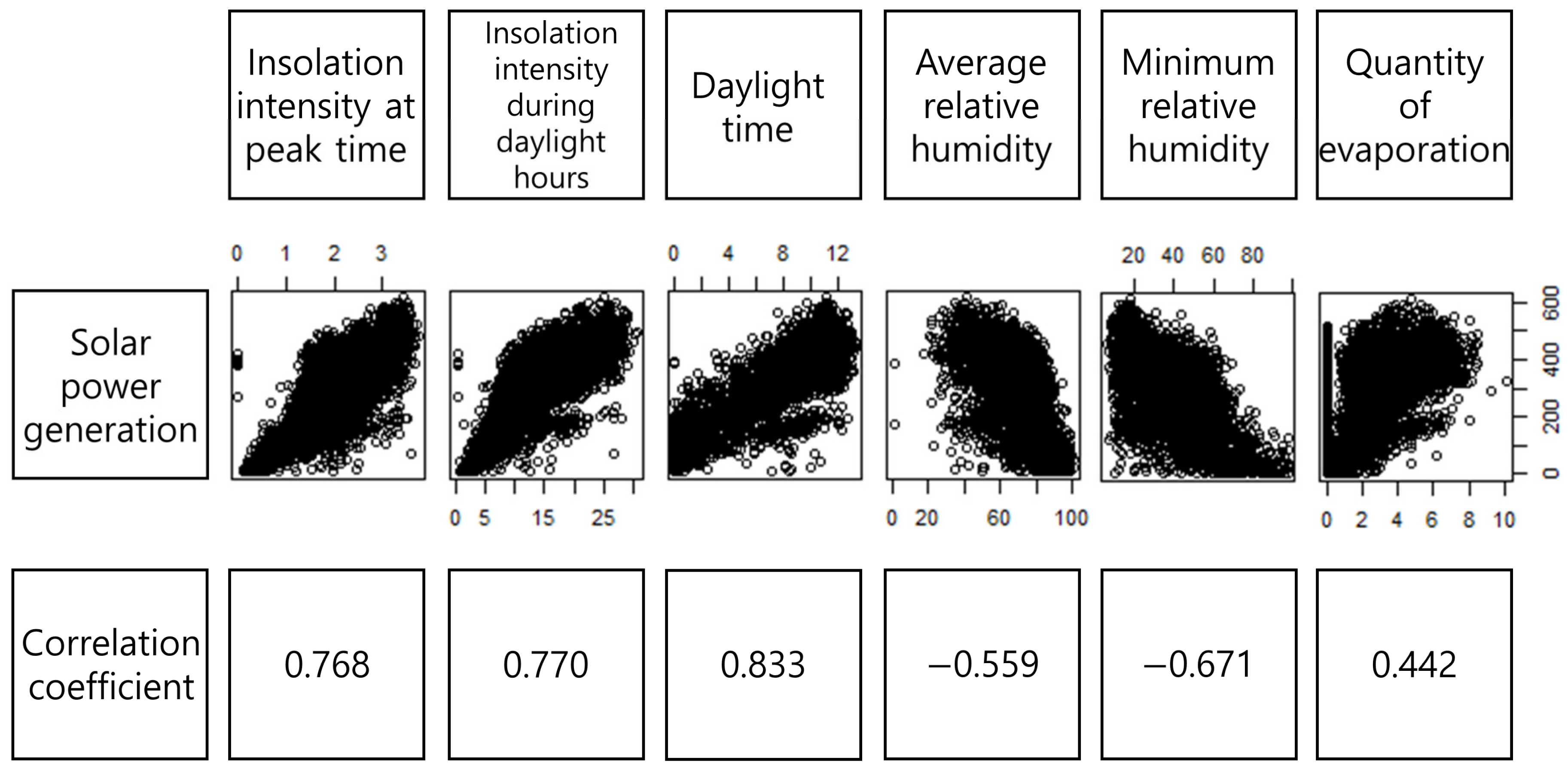
The meteorological variables considered for analyses were the insolation intensity at the peak time (MJ/m2), insolation intensity during daylight hours (MJ/m2), daylight time (h), average relative humidity (%), minimum relative humidity (%), and amount of evaporation (mm). The total number of meteorological data collected from January 2011 to December 2019 was 19,623 [27]. The numbers of data for the variables “daylight time”, “average relative humidity”, and “minimum relative humidity” were each 3285. The numbers of data for the variables “insolation intensity at the peak time” and “insolation intensity during daylight hours” were each 3281. The number of data for the variable “amount of evaporation” was 3206. Figure 3 shows the degrees of correlation between solar power generation and the several selected independent variables [28,29]. Figure 4 shows the degrees of correlation between the power generation and meteorological variables for the data sets collected over 9 years (2011–2019). As shown in Figure 4, three variables—i.e., the insolation intensity at the peak time, insolation intensity during daylight hours, and the daylight time—were highly positively correlated with power generation.

2.3. Analysis Method

In this paper, a multilinear regression analysis was applied to determine the causal relationship between independent variables (Xi), meteorological data, dependent variables (Y), and solar power generation because there were several independent variables. The regression analysis estimated the value of a dependent variable by substituting the values of independent variables. Accordingly, solar power generation can be estimated using a multilinear regression equation of the multiple meteorological variables as follows [30,31]:
( Y i ) = β 0 + β 1 X 1 i + β 2 X 2 i + + β p X p i
Equation (1) estimates the value of the dependent variable, as well as the values of the regression coefficients, β 0 ,   β 1 , β 2 , … and β p . Each regression coefficient is interpreted as the extent to which each independent variable affects the dependent variable.
Estimating regression coefficients requires partial differentiation of the error sum of squares (SSE) for each variable and minimizing it to estimate the regression variables. The SSE is represented as follows:
SSE = i = 1 m e i 2 = e 1 2 + e 2 2 + + e n 2 ,      
where e i is the deviation of the regression estimation.
In the regression analysis, the coefficient of determination ( R 2 ) is used to evaluate the goodness of fit or to know the explanatory power of the independent variables for estimating the dependent variable. The coefficient of determination is given as follows:
R 2 =   ( y i ^ y ¯ )   ( y i y ¯ ) 2 = V a r i a t i o n   e x p l a i n e d   b y   t h e   r e g r e s s i o n   l i n e T o t a l   v a r i a t i o n      
where y i ^ y ¯ indicates the difference between the estimated dependent variable value and sample mean.
The range of R 2 is 0 < R 2 < 1 . The closer it is to 1, the closer the regression model is to the overall variation. However, because multiple regression analysis has two or more independent variables, it is necessary to consider the adjusted coefficient of determination (Adjusted R 2 ), which compensates for the characteristic of R 2 that increases as the number of independent variables increases. The formula for the adjusted coefficient of determination is as follows:
Adjusted   R 2 = 1 n 1 ( n p 1 ) ( 1 R 2 )                                
where (np − 1) is the degree of freedom, n is the number of samples, and p is the number of independent variables.
In addition, the p-value and multicollinearity were diagnosed to confirm statistical significance. Finally, to evaluate the accuracy of the derived regression model, we used the R 2 , adjusted R 2 , and root mean square error (RMSE) values.
The p-value and probability of significance can determine if the null hypothesis or alternative hypothesis is adopted. To reject the null hypothesis that “the independent variables do not affect the dependent variable,” the p-value must be less than 0.05, and the alternative hypothesis can be adopted by rejecting the null hypothesis.
A multicollinearity between variables exists, which overlaps with the variability between independent variables and does not bring about overlapping variability. This leads to poor interpretation of the regression analysis results and decreases its accuracy, which requires diagnosis. Methods for diagnosing multicollinearity should utilize variance inflation factors (VIFs). VIFs can be determined using Equation (5) [32].
V I F i = 1 1 R 2
If the VIF is greater than 10, then the variable possesses multicollinearity and should be excluded from the regression analysis.
The RMSE is commonly used when considering the difference between the estimated and measured values, and it is suitable for expressing precision. The smaller the error, the better the performance of the regression model.

3. Results and Discussion

The coefficients of the entire regression model between the solar power generations over a year for the past 9 years and the meteorological variables are listed in Table 2. As observed in Table 2, the VIF values for the two independent variables—namely the insolation intensities at the peak time and during daylight hours—exceed 10. This indicates that these two variables possessed multicollinearity. Thus, the insolation intensity at the peak time was excluded from the regression model.
The revised regression models and their statistics were obtained after removing the insolation intensity at peak times, as summarized in Table 3 and Table 4, respectively. For the regression models given in Table 3, R 2 and adjusted R 2 were 0.7738 and 0.7735, respectively. The p-value is generally interpreted as statistically significant when it is less than 0.05. As the p-value is less than 0.05, the null hypothesis can be rejected, and the alternative hypothesis can be adopted [33]. In other words, the equation using coefficients in Table 3 can be used as a multiple linear regression model.
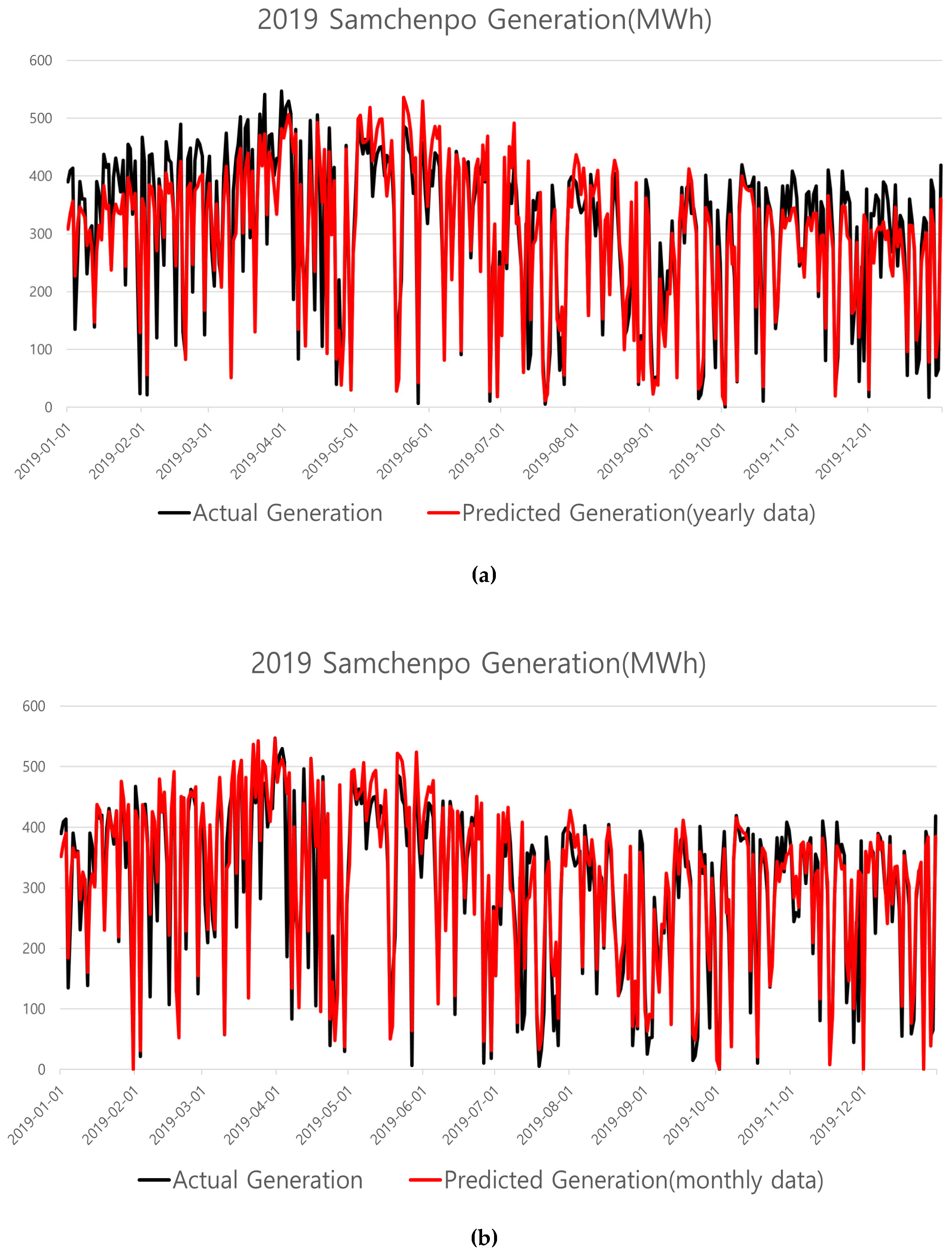
To consider the difference in monthly insolation, we derived 12 monthly regression models. Table 5 lists the regression models for the monthly solar power generation, which was averaged from 2011 to 2019. The R2s for the monthly regression models in Table 5 are larger than in Table 4. This means that the goodness of fit of the regression models in Table 5 was better than that of the regression model in Table 4. Therefore, the monthly regression models estimated solar power generation was better than the entire regression model. The regression model with the highest accuracy was for January and that with the lowest accuracy was for December. Figure 5 compares the actual daily power generation of the Samcheonpo power plant in 2019, as well as the predicted monthly regression models in Table 5.
Table 5 also shows that the two variables (insolation intensity during daylight hours (X1), and daylight time (X2)) were the dominant variables impacting the solar power generation. For January, June to September, and November to December, the insolation intensity during daylight hours (X1) was the most dominant meteorological variable. For February to May and October, the daylight times (X2) were the most dominant meteorological variable. Interestingly, the evaporation quantity fairly impacted solar power generation in January and November.

4. Conclusions

This study investigated the correlation between solar power generation and the meteorological variables by deriving multiple linear regression models. For this, a large data analysis software, R, was applied to the solar power generation and meteorological variable datasets. In the regression models, solar power generation was set as the dependent variable and the meteorological variables as the independent variables. The independent variables first considered were the insolation intensity at the peak time (MJ/h), insolation intensity during daylight hours (MJ/m2), daylight time (h), average relative humidity (%), minimum relative humidity (%), and evaporation amount (mm). Through statistical analysis, the insolation intensity at the peak time was excluded from the further regression model as it possessed multicollinearity. For the resulting regression model, R 2 was 0.7738, adjusted R 2 was 0.7735, and RMSE was 69.06.
In addition, 12 monthly regression models were derived to improve the predictability because the difference in monthly insolation had to be considered. The regression model with the highest accuracy was for January, with R 2 being 0.8985, adjusted R 2 being 0.8966, and RMSE being 40.66. The regression model with the lowest accuracy was for December, with R 2 being 0.7228, adjusted R 2 being 0.7178, and RMSE being 68.39. To check the predictability of the regression models, comparison between the actual daily power generation and the predicted power generation by the monthly regression models was shown in Figure 5.
Regression analyses showed the degree of correlation between solar power generation and each meteorological variable. The effect of each meteorological variable on solar power generation varied month-to-month. Among the two meteorological variables, the insolation intensity during daylight hours and daylight time had the highest correlation with solar power generation throughout the year. Interestingly, the quantity of evaporation impacted the solar power generation in January and November in a fairly big way.
This paper presented improved predictability for regression models by deriving the 12 monthly models used to consider the difference in monthly conditions of meteorological variables. Accordingly, we assumed that the predictability of the regression analysis for the data, including the variables, significantly varied month-to-month and could be improved by deriving monthly regression models rather than deriving an entire regression model.

Author Contributions

Formal analysis, Y.S.K. and H.Y.J.; Investigation, J.W.K.; Project administration, J.H.M.; Validation, H.Y.J., J.W.K. and S.Y.J.; Visualization, S.Y.J.; Writing—original draft, Y.S.K.; Writing—review & editing, J.H.M. All authors have read and agreed to the published version of the manuscript.

Funding

This research was funded by the National Research Found of Korea (NRF), grant number 2020M2D2A2062436, and by the Korea Foundation of Nuclear Safety (KoFONS), grant number 2003019.

Institutional Review Board Statement

Not applicable.

Informed Consent Statement

Not applicable.

Data Availability Statement

The data presented in this study are available on request from the corresponding author.

Acknowledgments

This work was supported in part by the National Research Foundation of Korea (NRF) grant funded by the Korea government (Ministry of Science and ICT). (No. 2020M2D2A2062436) and in part by the Nuclear Safety Research Program through the Korea Foundation of Nuclear Safety (KoFONS) using the financial resource granted by the Nuclear Safety and Security Commission (NSSC) of the Republic of Korea (No. 2003019).

Conflicts of Interest

The authors declare no conflict of interest.

References

  1. Korea Power Exchange. Power Generation Facility Status in 2019; Korea Power Exchange: Naju, Korea, 2020. [Google Scholar]
  2. Ministry of Trade, Industry and Energy. Implementation Plan for Renewable Energy 3020; Korea Government: Sejong, Korea, 2017.
  3. Kim, S.H.; Kim, S.W.; Seong, B.H.; Lee, G.M.; Oh, S.B.; Hwang, C.G. Relation between Module Temperature and Power in the 1 MW Rooftop Photovoltaic Power Plant. Trans. Korean Inst. Elect. Eng. 2014, 12, 154–155. [Google Scholar]
  4. Korea Meteorological Administration. Weather Resource Analysis Report for Optimal Utilization of Solar Energy; Korea Meteorological Administration: Seoul, Korea, 2008.
  5. de Freitas Viscondi, G.; Alves-Souza, S.N. A Systematic Literature Review on Big Data for Solar Photovoltaic Electricity Generation Forecasting. Sustain. Energy Technol. Assess. 2019, 31, 54–63. [Google Scholar] [CrossRef]
  6. Wolff, B.; Lorenz, E.; Kramer, O. Statistical Learning for Short-Term Photovoltaic Power Predictions. Stud. Comput. Intell. 2016, 645, 31–45. [Google Scholar]
  7. Ruiz-Arias, J.A.; Alsamamra, H.; Tovar-Pescador, J.; Pozo-Vázquez, D. Proposal of a Regressive Model for the Hourly Diffuse Solar Radiation under All Sky Conditions. Energy Convers. Manag. 2010, 51, 881–893. [Google Scholar] [CrossRef]
  8. Chen, B.; Lin, P.; Lai, Y.; Cheng, S.; Chen, Z.; Wu, L. Very-Short-Term Power Prediction for PV Power Plants Using a Simple and Effective RCC-LSTM Model Based on Short Term Multivariate Historical Datasets. Electronics 2020, 9, 289. [Google Scholar] [CrossRef] [Green Version]
  9. Benmouiza, K.; Cheknane, A. Small-Scale Solar Radiation Forecasting Using ARMA and Nonlinear Autoregressive Neural Network Models. Theor. Appl. Climatol. 2016, 124, 945–958. [Google Scholar] [CrossRef]
  10. Hossain, M.S.; Mahmood, H. Short-Term Photovoltaic Power Forecasting Using an LSTM Neural Network and Synthetic Weather Forecast. IEEE Access 2020, 8, 172524–172533. [Google Scholar] [CrossRef]
  11. Kalogirou, S.A. Artificial Neural Networks in Renewable Energy Systems Applications: A Review. Renew. Sustain. Energy Rev. 2001, 5, 373–401. [Google Scholar] [CrossRef]
  12. Lee, D.H.; Kim, K.H. Deep Learning Based Prediction Method of Long-term Photovoltaic Power Generation Using Meteorological and Seasonal Information. J. Soc. e-Bus. Stud. 2019, 24, 1–16. [Google Scholar]
  13. Lee, K.H.; Son, H.G.; Kim, S. A Study on Solar Energy Forecasting Based on Time Series Models. Korean J. Appl. Stat. 2018, 30, 139–153. [Google Scholar]
  14. Jeong, J.H.; Chae, Y.T. Improvement for Forecasting of Photovoltaic Power Output Using Real Time Weather Data Based on Machine Learning. J. Korean Soc. Living Environ. Sys. 2018, 25, 119–125. [Google Scholar] [CrossRef]
  15. Johnson, J.W. A Heuristic Method for Estimating the Relative Weight of Predictor Variables in Multiple Regression. Multivar. Behav. Res. 2000, 35, 1–19. [Google Scholar] [CrossRef]
  16. Muenchen, R.A. The Popularity of Data Analysis Software. R4Stats.Com 2012, No. April. Available online: http://r4stats.com/articles/popularity/ (accessed on 11 February 2021).
  17. Lee, G.H.; Lee, G.J.; Gang, S.W. Power Plant Location Analysis and Selection for Efficient Solar Energy Production. Korean Energy Econ. Rev. 2018, 17, 53–87. [Google Scholar]
  18. Jo, D.K.; Kang, Y.H.; Auh, C.M. A Study on the Analysis of Solar Radiation Characteristics on a High Elevated Area. J. Korean Solar Energy Soc. 2003, 23, 23–28. [Google Scholar]
  19. Korea Southeast Power Co. Ltd. Available online: https://www.koenergy.kr/kosep/hw/gv/nf/nfhw37/main.do?menuCd=GV050201 (accessed on 21 January 2021).
  20. Korea Central Power Co. Ltd. Available online: https://www.komipo.co.kr/kor/content/36/main.do?mnCd=FN021109 (accessed on 21 January 2021).
  21. Korea Southern Power Co. Ltd. Available online: https://www.kospo.co.kr/kospo/111/subview.do (accessed on 21 January 2021).
  22. Korea East-West Power Co. Ltd. Available online: https://ewp.co.kr/kor/subpage/contents.asp?cn=1314FD2O&ln=OO69QUWU&sb=UJ2MZMM2&tb=2ZWNPNL (accessed on 21 January 2021).
  23. Korea Western Power Co. Ltd. Available online: https://www.iwest.co.kr/iwest/559/subview.do (accessed on 21 January 2021).
  24. Korea Southeast Power Co. Ltd. Available online: https://www.koenergy.kr/kosep/hw/fr/ov/ovhw25/main.do?menuCd=FN0305010102 (accessed on 21 January 2021).
  25. Korea Southeast Power Co. Ltd. Available online: https://www.koenergy.kr/kosep/hw/br/sp/sphw04/main.do?menuCd=BR010203 (accessed on 21 January 2021).
  26. Korea Institute of Energy Research. Solar Energy Data Reference Standard Detailed Evaluation Procedure; Korea Institute of Energy Research: Daejeon, Korea, 2010. [Google Scholar]
  27. Korea Meteorological Administration. Available online: https://data.kma.go.kr/cmmn/main.do (accessed on 4 February 2021).
  28. Ministry of Public Administration and Security Information Disclosure System. Available online: https://www.open.go.kr/com/main/mainView.do?mainBgGubun=search (accessed on 4 February 2021).
  29. Sousa, S.I.V.; Martins, F.G.; Alvim-Ferraz, M.C.M.; Pereira, M.C. Multiple Linear Regression and Artificial Neural Networks Based on Principal Components to Predict Ozone Concentrations. Environ. Model. Softw. 2007, 22, 97–103. [Google Scholar] [CrossRef]
  30. Kang, S.H. Introductory Statistic; Free Academy Publishing: Paju, Korea, 2012; pp. 456–494. [Google Scholar]
  31. Kang, H.G. Statistical Methods for Healthcare Research, 6th ed.; Koonja Publishing: Paju, Korea, 2017; pp. 315–344. [Google Scholar]
  32. David, M.L. Statistics for Managers Using Microsoft Excel, 5th ed.; Pearson Prentice Hall Pulbishing: Upper Saddle River, NJ, USA, 2018; pp. 613–644. [Google Scholar]
  33. Kim, J.H. Environmental Statistics & Data Analysis; Hannarae Publishing: Seoul, Korea, 2018; pp. 205–269. [Google Scholar]
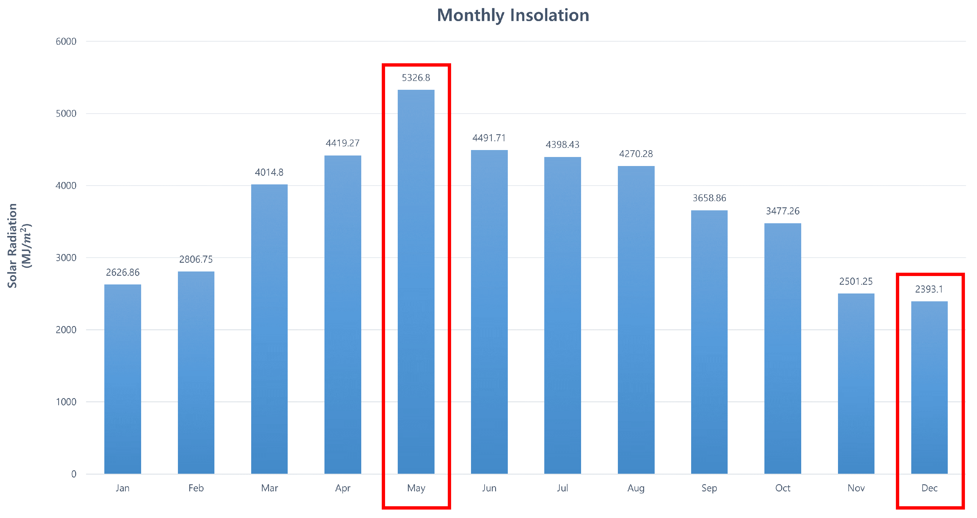
Figure 1. Monthly insolation (MJ/m2) averaged for the 9 years from 2011 to 2019.
Applsci 11 01776 g001
Figure 2. Location (white star in red cone) of Samcheonpo solar power plants [19,20,21,22,23].
Applsci 11 01776 g002
Figure 3. Degrees of correlation between solar power generation and several independent variables [27,28,29].
Applsci 11 01776 g003
Figure 4. Distributions of solar power generation and several meteorological variables over 9 years from 2011 to 2019.
Applsci 11 01776 g004
Figure 5. Comparison of the actual and the predicted solar power generations in 2019: (a) predicted by the regression model for the entire yearly data; (b) predicted by the 12 monthly regression models.
Applsci 11 01776 g005
Table 1. Overview of Samcheonpo solar power plants [24,25].
Facility Capacity
(MegaWatt)
Operation DateType
Samcheonpo #10.1October 2005 80 Wp × 1320  
Samcheonpo #20.99April 2010 225 Wp × 4400  
Samcheonpo #30.35April 2012 250 Wp × 1400  
Samcheonpo #41.85June 2012 250 Wp × 7400  
Samcheonpo #510.587June 2017 320 Wp × 33,000
Table 2. Multiple linear regression model for the yearly data collected over the past 9 years (2011–2019).
Coefficient
( β i )
Std. Errorp-ValueVIF
Constant174.978.48 2.2 × 10 16 -
Insolation intensity at peak time (MJ/m2)49.734.99 2.2 × 10 16 13.14
Insolation intensity during daylight hours (MJ/m2)4.420.75 4.5 × 10 9 18.61
Daylight time (h)13.640.67 2.2 × 10 16 4.87
Average relative humidity (%)−1.300.16 2.9 × 10 16 4.21
Minimum relative humidity (%)−0.740.15 6.7 × 10 16 6.06
Quantity of evaporation (kg/h)−9.000.87 2.2 × 10 16 2.24
Table 3. Revised multiple linear regression model for the yearly data collected over the past 9 years.
Coefficient
( β i )
Std. Errorp-ValueVIF
Constant201.918.16 2.2 × 10 16 -
Insolation intensity during daylight hours (MJ/m2) (X1)10.920.37 2.2 × 10 16 4.48
Daylight time (h) (X2)12.280.67 2.2 × 10 16 4.67
Average relative humidity (%) (X3)−1.080.16 1.1 × 10 11 4.13
Minimum relative humidity (%) (X4)−1.090.15 7.5 × 10 14 5.70
Quantity of evaporation (mm) (X5)−9.830.88 2.2 × 10 16 2.22
Table 4. Statistical test results of the revised regression model for the yearly data (2011–2019).
R2Adjusted R2RMSEStd. Error
0.77380.773569.0669.13
Table 5. Multiple linear regression models for each month.
Regression ModelR2Adjusted
R2
RMSEStd. Error
Const β 1 β 2 β 3 β 4 β 5
January55.1628.0812.19−1.991.24−17.700.89850.896640.6641.11
February94.3314.9221.20−1.830.93−4.070.86970.867153.9754.63
March104.809.5921.92−0.65−0.320.540.89160.889651.5952.15
April138.869.6315.91−0.54−0.87−3.390.87670.874459.9060.58
May104.789.5212.570.03−0.97−1.950.81420.810863.6664.35
June128.079.915.650.86−2.281.330.83000.826854.9355.55
July−102.314.762.322.76−1.61−4.700.77670.772660.5561.21
August−75.5016.51−3.601.96−1.231.980.77690.772855.0655.66
September−101.813.429.881.61−0.25−0.320.78420.780162.4263.12
October92.7411.0115.23−0.40−0.70−2.490.79520.791461.5762.43
November18.8428.623.35−0.12−0.35−21.750.745650.7408464.9465.67
December−103.533.676.040.320.38−1.280.72280.717868.3969.14
Publisher’s Note: MDPI stays neutral with regard to jurisdictional claims in published maps and institutional affiliations.