Abstract
Word sense disambiguation (WSD) is one of the core problems in natural language processing (NLP), which is to map an ambiguous word to its correct meaning in a specific context. There has been a lively interest in incorporating sense definition (gloss) into neural networks in recent studies, which makes great contribution to improving the performance of WSD. However, disambiguating polysemes of rare senses is still hard. In this paper, while taking gloss into consideration, we further improve the performance of the WSD system from the perspective of semantic representation. We encode the context and sense glosses of the target polysemy independently using encoders with the same structure. To obtain a better presentation in each encoder, we leverage the capsule network to capture different important information contained in multi-head attention. We finally choose the gloss representation closest to the context representation of the target word as its correct sense. We do experiments on English all-words WSD task. Experimental results show that our method achieves good performance, especially having an inspiring effect on disambiguating words of rare senses.
1. Introduction
Word sense disambiguation (WSD) with the ability to select the correct meaning of polysemous words depending on its language surroundings, has been considered one of the most difficult tasks in artificial intelligence [1]. As an “intermediate task”, the inefficiency of WSD stalls some related natural language processing (NLP) tasks to some extent. Some scholars have revealed its positive impact on improving the performance of downstream NLP tasks, i.e., information retrieval [2], machine translation [3,4], sentiment analysis [5], etc.
There are generally three approaches of WSD: knowledge-based methods, supervised methods, and unsupervised methods. Various lexical sources like WordNet and BabelNet are used as the knowledge bases for knowledge-based methods to determine the word meaning. Lesk [6] and its extended algorithms based on context-gloss overlap such as adapted Lesk [7] and enhanced Lesk [8] are typical of this method. Unsupervised methods usually use clustering method for disambiguation without any manual annotation of corpus. Graph-based algorithms [9] are applied to cluster features from texts. Supervised methods rely on manually labeled datasets. Research of the method focuses on extracting features. Researchers train a dedicated classifier for every target word exploiting support vector machine (SVM) models or other machine learning algorithms [10,11] in this method.
Recently, pre-trained models e.g., Context2Vec [12], ELMo [13], and BERT [14], have shown effectiveness on improving downstream NLP tasks. In this way, NLP task is to some extent divided into two parts: pretrain model to generate contextualized word representations and fine-tune model on downstream specific NLP task or directly use the pretrained word embedding. This motivates studies on WSD. In [15], authors explore different strategies to incorporate the contextualized word presentation for WSD. Work in [16] fine-tunes the pretrained BERT model to do the WSD task. A great number of other neural-based methods using a neural network encoder to extract features are proposed [17,18,19,20,21]. These methods bring further improvements. Among them, some studies incorporate the sense definitions information into their systems, proving glosses are helpful to improve performance of less frequent senses (LFS) words during training [16,18,19,20]. Even so, poor performance on rare or unseen senses remains a major obstacle in WSD.
This paper dedicates to improve WSD performance especially on LFS words. Our work follows closely prior works. We encode each polysemy and its senses independently using the same architecture and then optimize the two part jointly in the same embedding space, which turns out to be promising [20]. On this basis, we expect to obtain more valuable embeddings through encoding words and senses. To capture more decontextualized information, we enrich the multi-head attention with capsule network which was originally proposed to solve some defects in Convolutional Neural Networks (CNN) architecture [22]. It is found that routing parameters can imply the importance of capsules. Inspired by this idea, we consider attention of different heads as low layer capsules and aggregate them into high layer ones to obtain important information from perspectives of different heads.
Consequently, our contributions are listed as follows: (1) We construct a new model composed of context module and sense glosses module, called BiCapAtt, in which each module consists of multi-head attention that is improved by capsule network. (2) We evaluate the model on five standardized English benchmark datasets and get almost all results improved. (3) We also do extensive evaluations on rare words and rare senses and we get 29.0% F1-score improvement on the less frequent senses compared with previous state-of-the-art work.
2. Related Work
The upsurge of neural networks has promoted the research on WSD. The key point of WSD based on a language model is that the model can predict a word embedding with consideration for the surrounding words. So, WSD is accomplished by assigning the sense which is closest to the predicted sense embedding to the ambiguous word such as [23]. Other neural-based systems use a probability distribution usually computed by a softmax function to directly classify and assign a sense to the target word [11,24,25].
Contextual representations of words [12,13,14] have contributed to the task of WSD. Method in [12] employ bidirectional Long Short-Term Memory (BiLSTM) to effectively learn general sentence context representation from a large corpus and then use a k-nearest-neighbor algorithm to tag the sense. Work in [15] uses nearest neighbor matching and linear projection of hidden layers to exploit BERT to do the WSD task. The GAS model proposed by [19] is the first to incorporate the glosses knowledge into a neural WSD model, overcoming the scarcity of sense-annotated data. EWISE (Extended WSD Incorporating Sense Embeddings) [20] overcomes the bottleneck that existing supervised WSD systems have weak capability of learning low-frequency senses of words by learning continuous sense embedding. GlossBert [16] also takes glosses knowledge into consideration and constructs context-gloss pairs as the more suitable input to BERT. A robust method for generating sense embeddings with full coverage of all WordNet senses is introduced in [21]. The method leverages contextual embeddings, glosses, and semantic networks to achieve the full coverage. A more recent system [26] uses BERT to learn context embedding and the capsule network to decompose word embedding into multiple morpheme-like vectors.
Works in [19,20] are similar to our work. In general, the three models all have a context module that converts the context of the target word into context embeddings, and a gloss module that leverages the gloss knowledge in WordNet to generate sense embeddings. However, we construct the modules and train the model in different ways. The GAS model [19] simply uses BiLSTM to generate the context embedding and sense embedding, then uses a memory module to calculate the inner relationship between context and each gloss. The EWISE model [20] uses a BiLSTM and a self-attention layer to generate the context embedding. As for the sense embedding, it learns to embed gloss text relying on knowledge graph embeddings supervising. They train the models in a pipelined manner. In our model, we initialize input sentence sequence as BERT embeddings, and then use the same architecture of incorporating the capsule routing to the multi-head attention to obtain more robust context embeddings and sense embeddings than the above two models. We briefly introduce the capsule network and multi-head attention in Section 2.1 and Section 2.2, respectively. In addition, we train the model in an end-to-end manner.
To address the issue of lacking a unified framework, a reliable unified evaluation framework is proposed [25]. The framework standardizes training corpora and the datasets, annotating all the datasets with the sense inventory in WordNet 3.0 [27] and develops a java scorer which uses the metric of F1 score to measure the performance of WSD systems. The experiment results reported in this paper are based on this framework to make a fair comparison.
2.1. Capsule Network
The capsule network [22] replaces the single neuron node of the traditional neural network with neuron vectors, and uses dynamic routing to train this network. One capsule consists of a group of neurons. Dynamic routing is used between two capsules to find which high-level capsule the output of each low-level capsule is most likely to contribute to. Besides, a novel non-linear function called squash is used to produce the output vectors. The max pooling operation in CNN only retains the most active neurons and passes them to the next layer, resulting in loss of valuable spatial information. While in the capsule network, the spatial information and object existence probability are encoded in the capsule vector: the length of the vector represents the probability of feature existence and the direction of the vector represents the posture information of the feature. When modeling spatial information, the traditional CNN needs to copy feature detectors, which reduces the efficiency of the model. Space-insensitive methods inevitably limited to rich text structures (such as storing word location information, semantic information, etc.) are difficult to encode text effectively. The capsule network improves the above two defects. Some researchers have applied the capsule network to NLP tasks like text classification [28] and relation extraction [29] and they achieve competitive results.
2.2. Multi-Head Attention
The essence of the attention mechanism [30] is to imitate the human visual attention mechanism, learn a weight distribution of image features, and then apply this weight distribution to the original features to provide different feature effects for subsequent tasks such as image classification and image recognition. Multi-head attention [31] divides the model into multiple heads to form multiple subspaces, allowing the model to pay attention to information in different directions. Some researchers try to improve the multi-head attention mechanism. Some methods leverage the routing algorithm in the capsule network to improve the information aggregation for multi-head attention and achieve good results on machine translation [32,33,34].
3. Methodology
3.1. All-Words Task Definition
Our model aims to solve the English all-words WSD task, where all the ambiguous words in a given sentence require to be disambiguated. We formally propose the definition of the task in this part. In the sentence sequence L , polysemes are the target words, each of which has candidate senses . Additionally, each sense is a gloss sequence . The purpose of the task is matching the most suitable sense for the target word according to its current context. We use the predefined sense inventory provided by WordNet 3.0 [27].
3.2. Model Details
In this subsection, we present the details of our model. An overview architecture is depicted in Figure 1. The model encodes the context and sense glosses of an ambiguous word separately, then scores each sense for the target word. The score is calculated by the dot product of contextual embedding from the context module and sense embedding from the sense glosses module. In fact, the encoders of the two modules are exactly the same. In other words, we generate the context embedding and sense embedding in the same way.
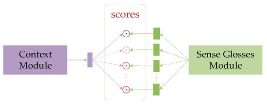
Figure 1.
Overview architecture of BiCapAtt.
Inspired by [33,34], we employ multi-head attention with the capsule network as our encoders. As illustrated in Figure 2, for an input sentence sequence, we initialize each word with BERT word embeddings as inputs of our model, where represents the length of the sequence and denotes the word embedding dimension.
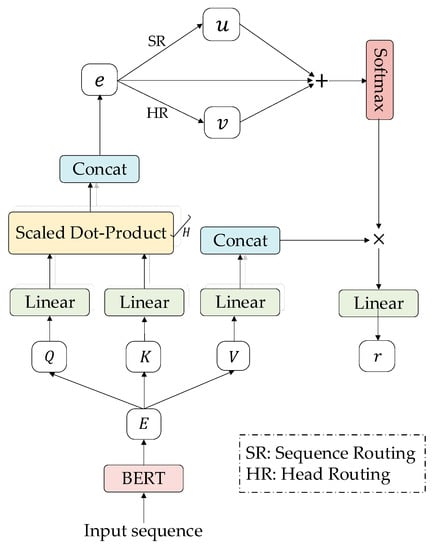
Figure 2.
The architecture of each module in BiCapAtt.
Multi-head attention used in transformer [29] focuses on information from various perspectives through splitting the model into multiple subspaces. The attention mechanism first projects the query , key and value to different subspaces with linear matrices as shown in Equation (1), where initially . Then, scaled dot-product for each head is calculated by Equation (2):
In the original capsule network, the input vector is multiplied by a pose matrix , which represents the spatial relationship between low-level features and high-level features. The result of multiplication is which indicates the high-level features derived from low-level features. The dynamic routing then is used to better determine the information added to the high-level capsules in the low-level capsules. In multi-head attention, the multiple attention heads can represent different partial information of the input sequence. We therefore treat them as low-level capsules, namely that already contain the spatial relationship. Figure 3 depicts the architecture of the capsule network. The dynamic routing algorithm (DR) we used is described in Algorithm 1.
| Algorithm 1 Dynamic Routing (DR). |
| Input: vectors , iteration times Process: 1. 2. for do 3. softmax computes Equation (3) 4. 5. squash computes Equation (4) 6. 7. end for Output: output vectors , weights |
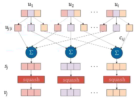
Figure 3.
The architecture of the capsule network.
There are input capsules and output capsules in Algorithm 1. Each input capsule will generate vectors and each vector will be assigned a weight value . First, the input vectors as the shallow capsules are weighted and added to get (Algorithm 1, Line 4). The weight is computed by:
where is initialized to zero and is updated as Algorithm 1, Lines 6. The softmax function can map multiple scalars into a probability distribution. Therefore, for each low-level capsule, its weight defines the probability distribution of the output belonging to each high-level capsule. Then, the non-linear function called squash is used to obtain the deep capsule vector, which is formulated as Equation (4). The squash function is mainly to make the length of not exceed 1, and keep and in the same direction. In this way, the length of the output vector is a number between 0 and 1, so the length can be interpreted as the probability that has a specific feature.
Taking advantage of the ability to recognize overlapping features of the capsule network, we incorporate the capsule routing into the multi-head attention to measure importance of information contained by various heads. Based on Equation (2), we see computed by Equation (5) as low layer capsules input to high layer capsules in the capsule network.
To attain deeper contextualized information, we consider the attention weight from two aspects: the sentence itself and the multiple heads. We call them sequence routing (SR) and head routing (HR), respectively. In the sequence routing, the capsules are as much as the heads and each capsule has L vectors, where L is the length of the sequence. The process of sequence routing is shown in Figure 4. We view as the input vectors. The input vectors generate output vectors and weights (indicated by the circle groups in Figure 4.) after the dynamic routing. The concat in figures means the concatenate operation. Considering heads have different effects on the output, softmax function is applied to the weights of each head for the sequence:
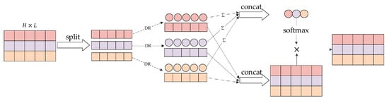
Figure 4.
The process of sequence routing.
The head routing is shown in Figure 5. There are capsules, and each capsule generates vectors in the head routing. We view as the input vectors. Taking measures to capture positional information among input tokens in the head routing is necessary because of its order dependence. Here, each capsule has a partial routing so that the sequential information is involved into the output capsules. Specifically speaking, the number of the head capsules is equal to the length of the sequence. For the capsule, its routing output is after the dynamic routing algorithm (Algorithm 1), which is computed by routing the top capsules. Then, we have the last head routing result computed as follows:
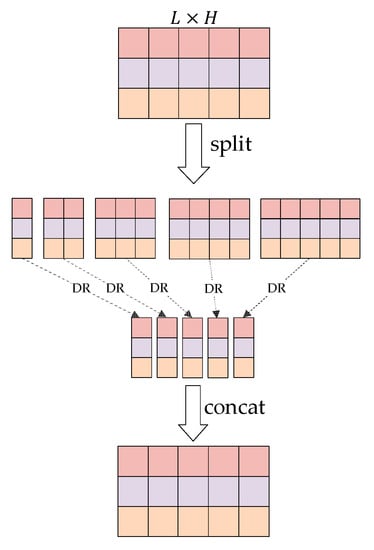
Figure 5.
The process of head routing.
At last, similar to a residual connection, we add to the sum of and . The sum of the three vectors is followed by a softmax function, which is multiplied by value to get the final output representations as follows:
In the context module, the encoder generates for input sequence, where is the length of context sequence. Because target words may be segmented into word pieces, we assume that target word corresponds to word list . We average representation to present the contextualized target word:
For each sense of the target word, the sense glosses module generates , where is the length of the current sense gloss. To identify the correct meaning, we score each sense simply by the dot product of word and its sense:
where denotes the sense inventory number of target word listed in WordNet. We choose the one who has the highest score as the most suitable sense of the polyseme. In the training process, parameters are updated by minimizing the cross-entropy loss on the scores:
4. Experiments
4.1. Datasets
Following previous work, we use SemCor 3.0 [35], the largest corpus to our knowledge manually annotated with WordNet sense, as training corpus. We exploit benchmark datasets proposed by [25] as evaluation datasets which include five standard all-words fine-grained WSD datasets and a concatenation of five datasets:
- Senseval-2 (SE2) [36];
- Senseval-3 (SE3) [37];
- SemEval-2007 (SE07) [38];
- SemEval-2013 (SE13) [39];
- SemEval-2015 (SE15) [40];
- ALL (the concatenation of above five datasets) [25].
We also choose the SE07 as our development set as most researchers do. Table 1 displays statistics about these datasets. The ambiguity reflects how difficult a dataset may be.

Table 1.
Statistics include the number of documents (Docs) and sentences (Sents) as well as the number of the sense annotations of noun (Noun), verb (Verb), adjective (Adj), adverb (Adv, and total of above four parts-of-speech (Total). The last column shows the ambiguity level of each dataset.
4.2. Experimental Setup
Our model is implemented in PyTorch. We use BERT (specifically, the model is bert-base-uncased) to get initial embeddings. The embedding dimension is 768. We set the number of attention heads to 8. The number of iterations in dynamic routing is 3 following original capsule network. The dropout probability is 0.1. The optimizer we used is Adam [41]. We explore a few learning rates, including , , , , , and , among which achieves the best. We set the batch size in the context module to 4, the batch size in sense glosses module to 256, the maximum length of the context is 128, and the maximum length gloss is 32. We train the model for 30 epochs and choose the model which has the best F1-score on the develop set during training. The total number of parameters of model reaches 853M. We use graphic processing unit (GPU) to accelerate computing. We do all the experiments on two Tesla V100-PCIE GPUs (NVIDIA, Santa Clara, CA, USA).
4.3. Results
4.3.1. Overall Results
Table 2 reports the F1 scores of our model and compares against previous different types of methods.
Table 2.
Reports of F1-score (%) on all-words word sense disambiguation (WSD) task, including SE07 (Dev), SE2, SE3, SE13, SE15, and ALL (concatenation of four test datasets) as well as every part-of-speech type (Noun, Verb, Adj, and Adv). Knowledge-based, traditional supervised, and neural-based methods and at last our method are listed. The best results are marked in bold and underlined numbers denotes previous state-of-the-art results.
We group systems by method type.
- Knowledge-based systems: The first four systems are knowledge-based methods, among which, MFS and WordNet S1 are two strong knowledge-based baselines. They select the most frequent sense (MFS) in the training dataset and in WordNet, respectively. Lesk+ext,emb [8] is an extended version of Lesk algorithm, which calculates the definition-context overlap to measure semantic similarity. Babelfy [42] builds a unified graph-based architecture that exploits BabelNet as the semantic network. WSD-TM [43] leverage the formalism of topic model to design a WSD system.
- Traditional supervised systems: IMS [10] and IMS+emb [11] are two traditional word expert supervised methods training an SVM classifier for WSD. The latter explores different approaches to incorporate word embeddings as features on the basis of the former using local features. The results show that word embeddings provide significant improvement.
- Neural-based systems: We list several recent neural-based methods. Bi-LSTM+att,LEX,POS [17] converts WSD to a sequence learning task. GASext (concatenation) [19] jointly encodes the context and glosses of the target word and extending gloss knowledge. EWISE [20] uses BiLSTM to train the context encoder and knowledge graph embedding to train the definition encoder. LMMS2348 (BERT) [21] focuses on making full use of WordNet knowledge to create sense-level embeddings. GlossBERT [16] constructs context-gloss pairs, thus treating WSD task as a sentence-pair classification problem to fine-tune the pre-trained BERT model. All the neural-based systems perform better than the traditional supervised and knowledge-based systems. It shows the ability of contextual representation and effectiveness of incorporating gloss knowledge. CapsDecE2S [26] utilizes capsule network to decompose the unsupervised word embedding into multiple morpheme-like vectors and merges them by contextual attention to generate context specific sense embedding. The CapsDecE2S and GlossBERT enable two strong baselines hard to beat.
Finally, we present the results of our system. To observe the results more intuitively, best score in each dataset is shown in bold and previous state-of-the-art results are underlined. As we can see in Table 2, our method shows promising results. Although the sources of the four datasets are extremely different which belongs to different domains, BiCapAtt achieves the best F1 score almost on every test dataset compared to other methods, outperforming the previous state-of-the-tart with 0.7% improvement on SE2, 3.3% on SE13, 1.5% on SE15, and 0.9% on ALL. Only the result on SE3 is 2.3% lower than that of CapsDecE2Slarge+LMMS. Besides, results on different part-of-speech (POS) type all achieve new state-of-the-art. Verbs and nouns usually have more senses than the other two parts-of-speech. The verbs show the worst performance in every system listed in Table 2 than other parts-of-speech because of its complexity of senses. From Table 1, we can see that SE07 holds the highest ambiguity level which has only verbs and nouns to be disambiguated. As a result, it shows worse performance than any other datasets in every system. Therefore, sense disambiguation for words with a great many of different meanings remains to be studied.
4.3.2. WSD on Rare Words and Rare Senses
We further compare the performance of several models on words with different frequency in the training dataset and on different frequency senses. For the former, we evaluate words that appear 0, 1 to 10, 11 to 50, and more than 50 occurrences during training. For the latter, we divide the ALL set into two subsets: the set of words labeled with most frequent sense (MFS), and the set of remaining words labeled with less frequent senses (LFS).
The F1 scores for different frequencies words in the training corpus are presented in Table 3. The high-frequency words usually have more senses, which leads to the worse performance. The previous methods show good performance on low-frequency words, but perform poorly on high-frequency words. Our model outperforms all the listed systems on unseen, rare, and frequent words.
Table 3.
F1-score (%) on words with different frequencies in the training corpus.
Table 4 shows the ability of our model to disambiguate words on LFS. We can find that the two knowledge-based methods have poor ability to recognize LFS. Compared to the EWISE, which predicts over sense embeddings enabling generalization to rare senses, our model improves the LFS subset by 29% F1-score with slightly improving the MFS subset. It proves the effectiveness of generating better presentation of contextual words and its sense definitions.
Table 4.
F1-score (%) on words labeled with most frequent sense (MFS) and words labeled with less frequent senses (LFS) of the ALL set.
4.4. Abaltion Study
To investigate the effects of the components of our model, we use the ALL set to perform an ablation study. As shown in Table 5, we first fine-tune the BERT-base by training a classifier, following by adding gloss module, multi-head attention mechanism (respectively with SR, HR, and both) based on the BERT-base baseline.
Table 5.
Ablation study on the ALL set.
It can be easily found that the improvement of LFS benefits from gloss knowledge a lot. Previous work [20] has also revealed this point. The gloss module allows the model to predict senses that do not occur in the train dataset by generating sense embeddings. In this way, it improves the performance of LFS.
We verify the effectiveness of SR and HR separately. Both routing parts work. The SR and HR alone can improve LFS performance with F1-score on MFS subtly decreased. Combining two routing achieves better results. It demonstrates that aggregation information from two separate perspectives is helpful. Our model is able to capture more useful information and thus obtain well representations.
5. Discussion
Our results are exciting for three main reasons. First, the BERT model shows its amazing power in many downstream NLP tasks. As an excellent pretrained model, it can provide deep contextual embedding. Recent works using BERT [11,19,38] have obtained very good results, and it is difficult to beat the method without BERT. We further extract deep features using capsule routing improved multi-head attention based on BERT embeddings. We regard the multiple groups of attention weights calculated by multi-head attention as capsules of different perspectives or capsules of subspaces. We then aggregate partial information carried by capsules through head routing and sequence routing. At last, we obtain a better sense representation. Even the infrequent senses can be well represented in our model. The last reason is the incorporation of glosses. We learn the sense embeddings independently, which improves the capability of zero-shot learning and thus helps disambiguating rare senses a lot.
6. Conclusions
This paper has introduced a supervised neural-based WSD method. Previous works have noticed the bottleneck of poor performance on rare and unseen senses and achieved inspiring results through making use of gloss knowledge. We manage to obtain better presentations while encoding context and sense glosses of target ambiguous word in the same space to improve LFS from a novel perspective. We leverage the advantage of capsule network to improve multi-head attention, thus obtain deeper contextual presentation. The experimental results on benchmark datasets prove that our method is effective and encouraging.
In this paper, we use the neural network architecture to encode the context and sense definition, which has room for improvement. In the future, we consider incorporating more relation such as hypernym and hyponym to enrich sense embeddings. Multilingual resources for improving sense embeddings will be another way taken into consideration. We also plan to apply our WSD model to downstream NLP tasks such as machine translation.
Author Contributions
Conceptualization, J.C. and W.T.; Methodology, J.C.; software, W.T.; validation, J.C., W.T., W.Y.; formal analysis, J.C.; investigation, J.C.; resources, W.T.; data curation, J.C.; writing—original draft preparation, J.C.; writing—review and editing, W.T., W.Y.; visualization, J.C.; supervision, W.T.; project administration, W.T.; funding acquisition, W.T. All authors have read and agreed to the published version of the manuscript.
Funding
This research was funded by the Shanghai Municipal Committee of Science and Technology, grant number 19511121002 and grant number 19DZ2252600, and by the Natural Science Foundation of Shandong Province, grant number ZR2019LZH002.
Conflicts of Interest
The authors declare no conflict of interest.
References
- Navigli, R. Word sense disambiguation: A survey. ACM Comput. Surv. 2009, 41, 1–69. [Google Scholar] [CrossRef]
- Zhong, Z.; Ng, H.T. Word sense disambiguation improves information retrieval. In Proceedings of the 50th Annual Meeting of the Association for Computational Linguistics, Association for Computational Linguistics, Jeju Island, Korea, 8–14 July 2012; pp. 273–282. [Google Scholar]
- Chan, Y.S.; Ng, H.T.; Chiang, D. Word sense disambiguation improves statistical machine translation. In Proceedings of the 45th Annual Meeting of the Association for Computational Linguistics, Prague, Czech Republic, 23–30 June 2007; pp. 33–40. [Google Scholar]
- Pu, X.; Pappas, N.; Henderson, J.; Popescu-Belis, A. Integrating Weakly Supervised Word Sense Disambiguation into Neural Machine Translation. Trans. Assoc. Comput. Linguist. 2018, 6, 635–649. [Google Scholar] [CrossRef][Green Version]
- Hung, C.; Chen, S.J. Word sense disambiguation based sentiment lexicons for sentiment classification. Knowl. Based Syst. 2016, 110, 224–232. [Google Scholar] [CrossRef]
- Lesk, M. Automatic Sense Disambiguation Using Machine Readable Dictionaries: How to Tell a Pine Cone from an Ice Cream Cone. In Proceedings of the 5th Annual International Conference on Systems Documentation, Toronto, ON, Canada, January 1986; pp. 24–26. [Google Scholar]
- Banerjee, S.; Pedersen, T. An Adapted Lesk Algorithm for Word Sense Disambiguation Using WordNet. In Proceedings of the International Conference on Intelligent Text Processing and Computational Linguistics, Mexico City, Mexico, 17–23 February 2002; pp. 136–145. [Google Scholar]
- Basile, P.; Caputo, A.; Semeraro, G. An Enhanced Lesk Word Sense Disambiguation Algorithm through a Distributional Semantic Model. In Proceedings of the COLING 2014, 25th International Conference on Computational Linguistics, Technical Papers, Dublin, Ireland, 23–29 August 2014; pp. 1591–1600. [Google Scholar]
- Sinha, R.; Mihalcea, R. Unsupervised graph-based word sense disambiguation using measures of word semantic similarity. In Proceedings of the International Conference on Semantic Computing, Irvine, CA, USA, 17–19 September 2007; pp. 363–369. [Google Scholar]
- Zhong, Z.; Ng, H.T. It Makes Sense: A Wide-Coverage Word Sense Disambiguation System for Free Text. In Proceedings of the ACL 2010 System Demonstrations, Uppsala, Sweden, 13 July 2010; pp. 78–83. [Google Scholar]
- Iacobacci, I.; Pilehvar, M.T.; Navigli, R. Embeddings for Word Sense Disambiguation: An Evaluation Study. In Proceedings of the 54rd Annual Meeting of the Association for Computational Linguistics, Berlin, Germany, 7–12 August 2016; pp. 897–907. [Google Scholar]
- Melamud, O.; Goldberger, J.; Dagan, I. context2vec: Learning Generic Context Embedding with Bidirectional LSTM. In Proceedings of the 20th SIGNLL Conference on Computational Natural Language Learning, Berlin, Germany, 11–12 August 2016; pp. 51–61. [Google Scholar]
- Peters, M.E.; Neumann, M.; Iyyer, M.; Gardner, M.; Clark, C.; Lee, K.; Zettlemoyer, L. Deep contextualized word representations. In Proceedings of the 2018 Conference of the North American Chapter of the Association for Computational Linguistics: Human Language Technologies, New Orleans, LA, USA, 1–6 June 2018; pp. 2227–2237. [Google Scholar]
- Devlin, J.; Chang, M.W.; Lee, K.; Toutanova, K. Bert: Pre-training of deep bidirectional transformers for language understanding. In Proceedings of the 2019 Conference of the North American Chapter of the Association for Computational Linguistics: Human Language Technologies, Volume 1 (Long and Short Papers), Minneapolis, MN, USA, 2–7 June 2019; pp. 4171–4186. [Google Scholar]
- Hadiwinoto, C.; Ng, H.T.; Gan, W.C. Improved Word Sense Disambiguation Using Pre-Trained Contextualized Word Representations. In Proceedings of the 2019 Conference on Empirical Methods in Natural Language Processing and the 9th International Joint Conference on Natural Language Processing, Hong Kong, China, 3–7 November 2019; pp. 5297–5306. [Google Scholar]
- Huang, L.; Sun, C.; Qiu, X.; Huang, X. Glossbert: Bert for word sense disambiguation with gloss knowledge. In Proceedings of the 2019 Conference on Empirical Methods in Natural Language Processing and the 9th International Joint Conference on Natural Language Processing, Hong Kong, China, 3–7 November 2019; pp. 3500–3505. [Google Scholar]
- Raganato, A.; Bovi, C.D.; Navigli, R. Neural sequence learning models for word sense disambiguation. In Proceedings of the 2017 Conference on Empirical Methods in Natural Language Processing, Copenhagen, Denmark, 9–11 September 2017; pp. 1156–1167. [Google Scholar]
- Luo, F.; Liu, T.; He, Z.; Xia, Q.; Sui, Z.; Chang, B. Leveraging gloss knowledge in neural word sense disambiguation by hierarchical co-attention. In Proceedings of the 2018 Conference on Empirical Methods in Natural Language Processing, Brussels, Belgium, 31 October–4 November 2018; pp. 1402–1411. [Google Scholar]
- Luo, F.; Liu, T.; Xia, Q.; Chang, B.; Sui, Z. Incorporating glosses into neural word sense disambiguation. In Proceedings of the 56th Annual Meeting of the Association for Computational Linguistics (Volume 1: Long Papers), Melbourne, Australia, 15–20 June 2018; pp. 2473–2482. [Google Scholar]
- Kumar, S.; Jat, S.; Saxena, K.; Talukdar, P. Zero-shot word sense disambiguation using sense definition embeddings. In Proceedings of the 57th Annual Meeting of the Association for Computational Linguistics, Florence, Italy, 28 July–2 August 2019; pp. 5670–5681. [Google Scholar]
- Loureiro, D.; Jorge, A. Language modelling makes sense: Propagating representations through WordNet for full-coverage word sense disambiguation. In Proceedings of the 57th Annual Meeting of the Association for Computational Linguistics, Florence, Italy, 28 July–2 August 2019; pp. 5682–5691. [Google Scholar] [CrossRef]
- Sabour, S.; Frosst, N.; Hinton, G.E. Dynamic routing between capsules. In Proceedings of the 31th Conference on Neural Information Processing Systems, Long Beach, CA, USA, 4–9 December 2017; pp. 3856–3866. [Google Scholar]
- Yuan, D.; Richardson, J.; Doherty, R.; Evans, C.; Altendorf, E. Semi-supervised word sense disambiguation with neural models. In Proceedings of the 26th International Conference on Computational Linguistics (COLING 2016), Osaka, Japan, 11–16 December 2016; pp. 1374–1385. [Google Scholar]
- Kageback, M.; Salomonsson, H. Word sense disambiguation using a bidirectional lstm. arXiv 2016, arXiv:1606.03568. [Google Scholar]
- Raganato, A.; Camacho-Collados, J.; Navigli, R. Word Sense Disambiguation: A Unified Evaluation Framework and Empirical Comparison. In Proceedings of the 15th Conference of the European Chapter of the Association for Computational Linguistics: Volume 1, Long Papers (EACL), Valencia, Spain, 3–7 April 2017; pp. 99–110. [Google Scholar]
- Liu, X.; Chen, Q.; Liu, Y.; Hu, B.; Siebert, J.; Wu, X.; Tang, B. Decomposing Word Embedding with the Capsule Network. Knowl. Based Syst. 2021, 212, 106611. [Google Scholar] [CrossRef]
- Miller, G. WordNet: An Electronic Lexical Database; MIT Press: Cambridge, MA, USA, 1998. [Google Scholar]
- Yang, M.; Zhao, W.; Ye, J.; Lei, Z.; Zhao, Z.; Zhang, S. Investigating Capsule Networks with Dynamic Routing for Text Classification. In Proceedings of the 2018 Conference on Empirical Methods in Natural Language Processing, Brussels, Belgium, 31 October–4 November 2018; pp. 3110–3119. [Google Scholar]
- Zhang, N.; Deng, S.; Sun, Z.; Chen, X.; Zhang, W.; Chen, H. Attention-Based Capsule Networks with Dynamic Routing for Relation Extraction. arXiv 2018, arXiv:1812.11321. [Google Scholar]
- Bahdanau, D.; Cho, K.; Bengio, Y. Neural machine translation by jointly learning to align and translate. arXiv 2014, arXiv:1409.0473. [Google Scholar]
- Vaswani, A.; Shazeer, N.; Parmar, N.; Uszkoreit, J.; Jones, L.; Gomez, A.N.; Kaiser, Ł.; Polosukhin, I. Attention is all you need. In Proceedings of the 31st International Conference on Neural Information Processing Systems, Long Beach, CA, USA, 4–9 December 2017; pp. 5998–6008. [Google Scholar]
- Li, J.; Yang, B.; Dou, Z.; Wang, X.; Lyu, M.R.; Tu, Z. Information Aggregation for Multi-Head Attention with Routing-by Agreement. In Proceedings of the 2019 Conference of the North American Chapter of the Association for Computational Linguistics: Human Language Technologies, Volume 1 (Long and Short Papers), New Orleans, LA, USA, 1–6 June 2019; pp. 3566–3575. [Google Scholar]
- Duan, S.; Cao, J.; Zhao, H. Capsule-Transformer for Neural Machine Translation. arXiv 2019, arXiv:2004.14649. [Google Scholar]
- Gu, S.; Feng, Y. Improving Multi-Head Attention with Capsule Networks. In Proceedings of the 8th Conferernce of Natural Language Processing and Chinese Computing, Dunhuang, China, 9–14 October 2019; pp. 314–326. [Google Scholar]
- Miller, G.A.; Chodorow, M.; Landes, S.; Leacock, C.; Thomas, R.G. Using a semantic concordance for sense identification. In Proceedings of the workshop on Human Language Technology, Plainsboro, NJ, USA, 8–11 March 1994; pp. 240–243. [Google Scholar]
- Edmonds, P.; Cotton, S. SENSEVAL-2: Overview. In Proceedings of the Second International Workshop on Evaluating Word Sense Disambiguation Systems, SENSEVAL ’01, Toulouse, France, 5–6 July 2001; pp. 1–5. [Google Scholar]
- Snyder, B.; Palmer, M. The english all-words task. Proceedings of SENSEVAL-3, the Third International Workshop on the Evaluation of Systems for the Semantic Analysis of Text, Barcelona, Spain, 25–26 July 2004; pp. 41–43. [Google Scholar]
- Pradhan, S.; Loper, E.; Dligach, D.; Palmer, M. Semeval-2007 task-17: English lexical sample, srl and all words. In Proceedings of the Fourth International Workshop on Semantic Evaluations (SemEval-2007), Prague, Czech Republic, 23–24 June 2007; pp. 87–92. [Google Scholar]
- Navigli, R.; Jurgens, D.; Vannella, D. Semeval-2013 Task 12: Multilingual Word Sense Disambiguation. In Proceedings of the Second Joint Conference on Lexical and Computational Semantics (* SEM), Volume 2 and the Seventh International Workshop on Semantic Evaluation (SemEval 2013), Atlanta, GA, USA, 14–15 June 2013; pp. 222–231. [Google Scholar]
- Moro, A.; Navigli, R. Semeval2015 task 13: Multilingual all-words sense disambiguation and entity linking. In Proceedings of the 9th International Workshop on Semantic Evaluation (SemEval 2015), Denver, CO, USA, 4–5 June 2015; pp. 288–297. [Google Scholar]
- Kingma, D.; Ba, J. Adam: A Method for Stochastic Optimization. arXiv 2014, arXiv:1412.6980. [Google Scholar]
- Moro, A.; Raganato, A.; Navigli, R. Entity linking meets word sense disambiguation: A unified approach. Trans. Assoc. Comput. Linguist. 2014, 2, 231–244. [Google Scholar] [CrossRef]
- Chaplot, D.S.; Salakhutdinov, R. Knowledge-based Word Sense Disambiguation using Topic Models. Proceedings of 30th Innovative Applications of Artificial Intelligence Conference, New Orleans, LA, USA, 2–7 February 2018; pp. 5062–5069. [Google Scholar]
Publisher’s Note: MDPI stays neutral with regard to jurisdictional claims in published maps and institutional affiliations. |
© 2021 by the authors. Licensee MDPI, Basel, Switzerland. This article is an open access article distributed under the terms and conditions of the Creative Commons Attribution (CC BY) license (http://creativecommons.org/licenses/by/4.0/).