Wankelmut: A Simple Benchmark for the Evolvability of Behavioral Complexity

Abstract

In evolutionary robotics, an encoding of the control software that maps sensor data (input) to motor control values (output) is shaped by stochastic optimization methods to complete a predefined task. This approach is assumed to be beneficial compared to standard methods of controller design in those cases where no a priori model is available that could help to optimize performance. For robots that have to operate in unpredictable environments as well, an evolutionary robotics approach is favorable. We present here a simple-to-implement, but hard-to-pass benchmark to allow for quantifying the “evolvability” of such evolving robot control software towards increasing behavioral complexity. We demonstrate that such a model-free approach is not a free lunch, as already simple tasks can be unsolvable barriers for fully open-ended uninformed evolutionary computation techniques. We propose the “Wankelmut” task as an objective for an evolutionary approach that starts from scratch without pre-shaped controller software or any other informed approach that would force the behavior to be evolved in a desired way. Our main claim is that “Wankelmut” represents the simplest set of problems that makes plain-vanilla evolutionary computation fail. We demonstrate this by a series of simple standard evolutionary approaches using different fitness functions and standard artificial neural networks, as well as continuous-time recurrent neural networks. All our tested approaches failed. From our observations, we conclude that other evolutionary approaches will also fail if they do not per se favor or enforce the modularity of the evolved structures and if they do not freeze or protect already evolved functionalities from being destroyed again in the later evolutionary process. However, such a protection would require a priori knowledge of the solution of the task and contradict the “no a priori model” approach that is often claimed in evolutionary computation. Thus, we propose a hard-to-pass benchmark in order to make a strong statement for self-complexifying and generative approaches in evolutionary computation in general and in evolutionary robotics specifically. We anticipate that defining such a benchmark by seeking the simplest task that causes the evolutionary process to fail can be a valuable benchmark for promoting future development in the fields of artificial intelligence, evolutionary robotics, and artificial life.

1. Introduction

Robots are used more and more frequently in inherently unpredictable outdoor environments: aerial search, rescue drones, deep-diving underwater AUVs, and even extra-terrestrial explorative probes. It is impossible to program autonomous robots for those tasks in a way that a priori accommodates all possible events that might occur during such missions. Thus, on-line and on-board learning, conducted for example by evolutionary computation and machine learning, becomes a significant aspect in those systems [1,2,3,4]. Evolutionary robotics has become a promising field of research to push forward the robustness, flexibility, and adaptivity of autonomous robots, which combines the software technologies of machine learning, evolutionary computation, and sensorimotor control with the physical embodiment of the robot in its environment.

We claim here that evolutionary robotics operating without a priori knowledge can fail easily because it suddenly hits an obscured “wall of complexity” with the current state-of-the-art of unsupervised learning. Extremely simple (trivial) tasks evolve well with almost every approach that was tested in literature [2,5,6,7]. However, already slightly more difficult tasks make all methods fail that are not a priori tailored to the properties that are needed to be able to evolve a solution for the software controller for the given task [2,7,8]. However, these are often unknown for black-box problems where evolutionary computation and evolutionary robotics are applied most usefully. As is well known, there is no free lunch in optimization techniques [9]. The more specifically an optimizer is tailored to a specific problem, the more probable it is that it will fail for other types of problems. Thus, only open-ended, uninformed evolutionary computation will allow for generality in problem solving as required in long-term autonomous operations in unpredictable environments. For example, many studies in the literature that have evolved complex tasks of cooperation and coordination in robots used pre-structured software controllers [6,10], while many studies that have evolved robotic controllers in an uninformed open-ended way produced only simple behaviors, such as coupled oscillators that generate gaits in robots [11,12,13,14] including simple reactive gaits [15], homing, collision avoidance, area coverage, collective pushing/pulling, and similar straight-forward tasks [16].

We hypothesize that one reason for the lack of success of evolving solutions for complex tasks is the improbable emergence of internal modularity [17] in software controllers using open-ended evolution without explicitly enabling the evolution of modules. In an evolutionary approach, it is possible to push towards modularity by pre-defining a certain topology of Artificial Neural Networks (ANNs) [18], by allowing evolving a potentially unlimited number of modules within a pre-defined modular ANN structure [19,20] or by switching between tasks on the time scale of generations [21], which can then also be improved by imposing costs for links between neurons [22]. However, if modularity is not pre-defined and not explicitly encouraged by a designer, then a modular software controller will not emerge from scratch even if modularity is directly required by the task. While nature is capable of evolving highly layered, modularized, and complex brain structures [23] by starting from scratch, evolutionary computation fails to achieve similar progress within a reasonable time.

To support our claim, we searched for the most simple task that leads to the failure of plain-vanilla uninformed unsupervised evolutionary computation starting from a 100% randomized control software without any interference (guidance) by a designer during evolution and without any a priori mechanism or impetus to favor self-modularization. An easy way to define such a task is to construct it from two simple, but conflicting tasks that are both easily evolvable in isolation for almost any evolutionary computation and machine learning approach of today. However, we require that the behavior that solves Task 1 is the inverse of the behavior that solves Task 2 (e.g., positive and negative phototaxis). Hence, once one behavior has been evolved, the other behavior needs to be added together with an action selection mechanism. We propose a task that operates in one-dimensional space, and as it is shown in the paper, it can be solved by a very simple pseudo-code and also by hand-coded ANNs. Compared to the classification scheme of Braitenberg [24], an agent that solves the Wankelmut (German, meaning roughly “whiffler”: a person who frequently changes opinions or course; see https://www.merriam-webster.com/dictionary/whiffler (accessed on 29 January 2021)) task would be placed between Vehicle #4 and Vehicle #5 concerning the complexity of its behavior. Given that it operates in a one-dimensional space, this introduces a relation to Vehicle #1. We anticipate that searching to define the definition of such a “most simple task to fail” is a valuable effort benchmark for promoting future development in the fields of artificial intelligence, evolutionary robotics, and artificial life.

For simplicity, we suggest simple plain-vanilla ANNs as an evolvable runtime control software in combination with genetic algorithms [25] or evolution strategies [26] as an unsupervised adaptation mechanism. For our benchmark defined here, we accept either large fully-connected and randomized ANNs as initialization, as well as ANN implementations that allow restructuring (adding and removing of nodes and connections) as a starting point. However, we consider all implementations that have special implementations to facilitate or favored modular networks as “inapplicable for our focal research question” because the main challenge in our benchmark task is to evolve modularization from scratch as an emergent solution to the task.

2. Our Benchmark Task

For the sake of simplicity, we restrict ourselves to a very simple task that is hard to evolve in an open-ended, uninformed, and unguided way. As shown in Figure 1, we assume an agent that moves in an environment expressing one single quality factor (e.g., height, water or air pressure, luminance, temperature) and that has to evolve a behavior that first makes the agent move uphill in this environmental gradient.

In the “uphill-walk” phase of the experiment, the agent always should move in the direction of the sensor that reports the higher value of the focal quality factor. As soon as the agent reaches an area of sufficiently high quality (above a threshold ${\Theta }_{max}$), the agent should switch its behavioral mode and start to seek areas of low environmental quality. In this “downhill-walk” phase, the agent should always move towards the side where its sensor reports the lowest environmental quality value. After the agent has reached a sufficiently low quality area (below a threshold ${\Theta }_{min}$), the agent should switch back to the “uphill-walk” behavior again.

We call the behavior that we aim to evolve “Wankelmut”, a term that expresses in German a character trait in which one always switches between two different goals as soon as one of the goals is reached. A “Wankelmut” agent is never satisfied and thus does not decide one thing and does not stick with it. It is a variant of “the grass is always greener,” a commonly found personality feature in natural agents (from humans to animals), and despite its negative perception in many cultural moral systems, it has its benefits. It keeps the agent going, being explorative, curious, and never satisfied. That is exactly the desired behavior of an autonomous probe on a distant planet that needs to be explored.

In summary, the task is to follow an environmental gradient up and down in an alternating way, hence maximizing the coverage (monitoring, observation, patrolling) of the areas between ${\Theta }_{min}$ and ${\Theta }_{max}$. There are many examples that have been evolved by natural selection [27]. In social insects (ants, termites, wasps, honeybees), foragers have first to go out of the nest, and after they encounter food, they switch their behavior and go back to the nest. After they have unloaded the food to other nest workers, they go outwards to forage again [28]. Often, environmental cues and gradients are involved in the homing and in the foraging behaviors (sun compass, nest scent, pheromone marks) and are exploited differently by the workers in the outbound behavioral state compared to the inbound behavioral state [29]. Other biological sources of inspiration are animals following a diurnal rhythm (day-walkers and night-walkers). In an engineering context, the rhythm might be imposed by energy recharging cycles, water depths, or aerial heights in transportation tasks by underwater vehicles or aerial drones.

Figure 1B shows that we de-complexified the benchmark task to a one-dimensional cellular space of N cells in which always one cell of index $P\left(t\right)$ is occupied by the agent that has state $S\left(t\right)$. The environmental gradient is produced by the Gauss error function:

$$erf\left(x\right)=\frac{2}{\sqrt{\pi }}{\int }_0^x{e}^{-t^2}\mathrm{dt},$$

(1)

whereby the quality of every cell i is modeled as:

$$\mathrm{quality}\left[i\right]=erf\left(\frac{4(i-\frac{N}{2})}{N}\right).$$

(2)

In every time step $t\in [0,t_{max}]$, the agent has access to two lateral sensor readings, which are modeled as:

$$s_l\left(t\right)=\left\{\begin{array}{cc}\mathrm{quality}\left[P\right(t)-1]\hfill & \mathrm{if}\left(P\right(t)>0)\hfill \\ \mathrm{quality}\left[P\right(t\left)\right]\hfill & \mathrm{otherwise}\hfill \end{array}\right.$$

(3)

and:

$$s_r\left(t\right)=\left\{\begin{array}{cc}\mathrm{quality}\left[P\right(t)+1]\hfill & \mathrm{if}\left(P\right(t)<N-1)\hfill \\ \mathrm{quality}\left[P\right(t\left)\right]\hfill & \mathrm{otherwise}\hfill \end{array}\right..$$

(4)

The agent changes its position based on these sensor readings:

$$P(t+1)=min(N-1,max(0,P\left(t\right)+f(s_l\left(t\right),s_r\left(t\right)))),$$

(5)

whereby the agent’s position is restricted by the boundaries of the simulated world. Its motion (f) is restricted to a maximum of one step to the left or to the right of the agent’s current position.

Initially, the agent is in the uphill, state which means it should move uphill. If the agent’s local $\mathrm{quality}\left[P\left(t\right)\right]\ge {\Theta }_{max}$, then the state is changed to downhill, and if the agent’s local $\mathrm{quality}\left[P\left(t\right)\right]\le {\Theta }_{min}$, then the agent’s state is changed back to uphill.

3. Known Solutions

The Wankelmut task is actually very simple to solve, as it is just a greedy uphill walk in combination with a greedy downhill walk complemented by a threshold-dependent switch.

A simple algorithm, such as the Python-like pseudo-code in Figure 2, solves the task with a few lines of code in the desired reactive and optimal way. We used this code to calculate the “maximum reachable fitness” in our Quantitative Analysis Section. The variable state and the constant theta define the agent’s own state and the thresholds at which it should switch from one behavior to the other and vice versa. The two variables S_l and S_r hold the current sensor values at the left and at the right side of the agent and report values between $-1.0$ and $+1.0$. The function set-actuators() drives the robot to the left with positive numbers and to the right with negative numbers used as the only argument. In our study, we use this simple hand-coded solution as a reference and investigate how close the evolved control software gets to the fitness values achieved by this simple, but optimal solution.

It is noteworthy that this reactive solution of the Wankelmut task would operate in gradients of any shape and size in an optimal way as long as gradients are strictly monotone between the two points ${\Theta }_{min}$ and ${\Theta }_{max}$. While we used a sigmoid-type non-linear gradient by using the Gauss error function, our hand-coded solution, presented as pseudo-code in Figure 2, works optimally also in linear gradients of any size and steepness.

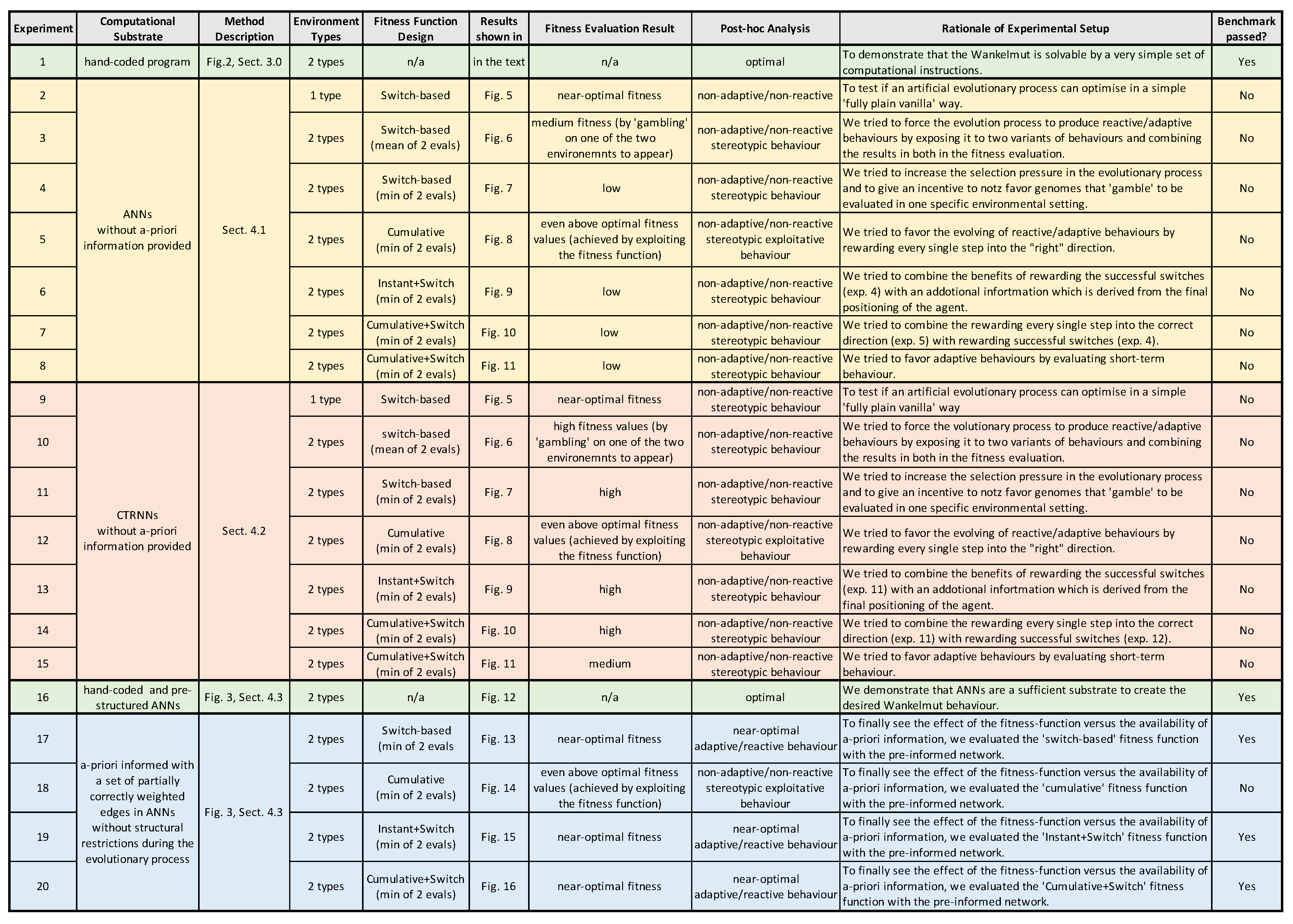
4. Evolvable Agent Controllers

In the following, we describe the different representations of robot controllers that we tested: simple artificial neural networks (Section 4.1), continuous-time recurrent neural networks (Section 4.2), and as a control experiment, also hand-coded artificial neural networks (Section 4.3). In Section 5, we present the results for all controller variants in two environments (mirrored gradient) for different fitness functions. For an overview, see Figure 3.

4.1. Simple Artificial Neural Network

Our simple approach made use of recurrent artificial neural networks. The activation function used is a sigmoid function:

$$1/(1+exp(-20x\left)\right)-0.5.$$

(6)

The network has eleven neurons distributed over the input layer (two), a first hidden layer (three), a second hidden layer (three), a third hidden layer (two), and the output layer (one). Each neuron in the second hidden layer has a link to itself (loop) and an input link from each of the neighboring nodes in addition to the links from the nodes in the previous layer. Weights were randomly initialized with a random uniform distribution from the interval $[-0.5,0.5]$.

4.2. Continuous-Time Recurrent Neural Networks

In a second approach, we used Continuous-Time Recurrent Neural Networks (CTRNNs), which are Hopfield continuous networks with an unrestricted weight matrix inspired by biological neurons [30]. A neuron i in the network is of the following general form:

$${\tau }_i\dot{y_i}=-y_i+\sum _{j=1}^N{w}_{ji}\sigma \left(g_j(y_j+{\theta }_j)\right)+I_i$$

(7)

where $y_i$ is the state of the ith neuron, ${\tau }_i$ is the neuron’s time constant, $w_{ji}$ is the weight of the connection from the jth to ith neuron, ${\theta }_i$ is a bias term, $g_i$ is a gain term, $I_i$ is an external input, and $\sigma \left(x\right)=1/(1+exp(-x\left)\right)$ is the standard logistic output function.

The weights were randomly initialized. By considering the study of the parameter space structure of the CTRNN by [31], the values of the $\theta$s were set based on the weights in a way that the richest possible dynamics were achieved. We used 11 nodes where two nodes received the sensor inputs and one node was used as the output node determining the direction of the movement (right/left).

4.3. Hand-Coded Artificial Neural Network

In order to make sure that the topology of our evolved neural networks is sufficient for solving the problem, we designed hand-coded neural network solutions that are based on the same topology as at least one of the networks described above (ANN or CTRNN).

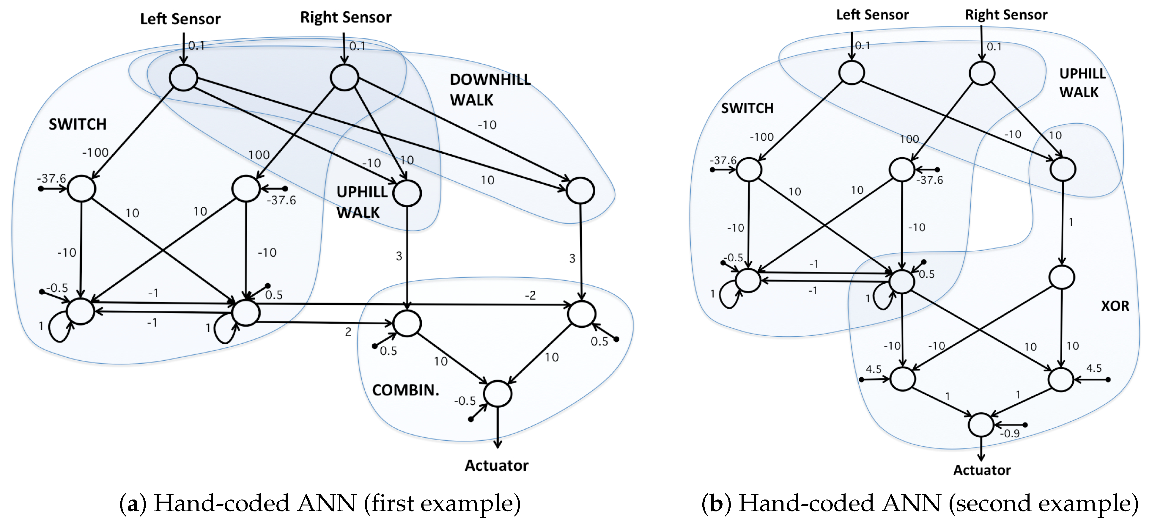
For the activation function, we used Equation (6), as before. Figure 4 shows two examples of hand-coded neural networks. The first example is topologically consistent with the CTRNN defined in the previous subsection. The second example is topologically consistent with both the ANN and CTRNN defined in the previous subsections. That means, in principle, it is possible for an evolutionary algorithm to evolve this problem from a population of the above ANNs or CTRNNs.

To design the hand-coded networks, we followed a logic based on subnetworks for various subtasks. In Figure 4a, an uphill and a downhill walk subnetwork and a switch subnetwork are designed. The switch keeps the current state of the controller, and when the inputs pass the thresholds, it switches to the other state. Finally, in the last subnetwork, the information from the switch is used to choose between uphill and downhill walk. Figure 4b has a slightly different design where the output of the switch and an uphill walk subnetwork are combined by using a logical XOR subnetwork. The number of the nodes in both networks is the same; however, the number of weights used in the second example is lower.

The behaviors of an agent controlled by both networks are the same. The behaviors in two different environments are demonstrated in Figure 5b,c. Figure 5b shows the behavior when the quality of the environment is increasing from left to right. Figure 5c shows the behavior when the quality of the environment is decreasing (the quality of the environments is represented in gray-scale).

In the next step, we allowed evolution to optimize the weights of the second hand-coded network. For that, we made a population of ANNs with the topology described in Section 4.1. The connection weights of the population were initialized with the weights of the second hand-coded network. The non-existing weights in the hand-coded network were set to zero in the population. The evolutionary algorithm was then allowed to change the weights including the ones with zero value. The details of the evolutionary algorithm and the results are described in Section 5.

4.4. What Do We Expect to See as a Solution to the Wankelmut Task?

Although the task might seem to be solved in a straight forward way, a number of different strategies can be taken by an optimal controller. Notice also that we tested our agents in two types of environments: one environment with the maximum at the left-hand side and another environment with the maximum at the right-hand side.

An intuitive solution is a controller that can go uphill or downhill along the gradient with a 1 bit internal memory for determining the current required movement strategy (uphill or downhill). The internal memory switches its state when the sensor values reach the extremes (defined thresholds). The initial state of the memory should indicate the uphill movement. Hence, a controller requires only this 1 bit internal memory. The comparison between the instant values of the sensors then determines the actual direction of the movement in each step. We would consider such a solution as a “correct” solution, as it basically resembles the pseudo-code given in Figure 2. We assume that our chosen topology of the ANNs allows in principle to evolve the required behavior based on one internal binary state variable. Our simple ANN was a recurrent network and had two hidden layers with three nodes each. These two hidden layers should have provided enough options to evolve an independent (modular) uphill and downhill controller in combination with a 1 bit memory and an action selection mechanism. Similarly, for the CTRNN approach, we have nine neurons, and any topology between them was allowed.

Another solution to solve the task can be done in the following way: The controller starts by deciding about the initial direction of the agent’s movement to the right or left depending on the initial sensor value. Following this, it continues a blind movement (i.e., not considering the directional information of the sensor inputs) until extreme sensor values are perceived and then switches the direction of the agent. Here also, an internal 1 bit state variable is required to keep the direction of the agent’s movement.

There is even another solution possible. As our environment does not change in size, the controller does not even need to consider the sensor values at any time except the first time step: In this strategy, the robot has to initially classify the environment, and then, the remaining task can be completed correctly by choosing one of two “pre-programmed” trajectories. In this solution, the sensor information is only used at the first time step, but then, a more complicated memory (more than 1 bit) is needed to maintain the oscillatory movement between the two extremes. This is not a maximally reactive solution meaning that it partially replaces reactivity to sensor inputs with other mechanisms; i.e., using extra memory and pre-programmed behaviors. Such a solution would not work in the way we expect it to work in other environments (e.g., changed size of the gradient). Such a controller might achieve the optimal fitness in our evolutionary runs, but a post-hoc test in a slightly different environment would identify that it generates sub-optimal behavior. Thus, it does not represent a valid solution for the Wankelmut task. A post-hoc test that detects such a solution could be done by changing the size or the steepness of the environmental gradient or by using a Gaussian function (bell curve) instead of the Gauss error function (erf) with randomized starting positions: in this case, the agent should oscillate only in the left or in the right half of the environment, depending on its starting position, to implement a true reactive solution to the Wankelmut task.

Other solution strategies can also concern the switching condition, for example the switching may occur based on the extreme values of the sensors (defined thresholds), the difference between the two sensor values, or the fact that at the boundaries of the arena, the sensor values may not change even if the agent attempts to keep moving in the same direction, as we do not allow the agent to leave the arena.

Here, we are interested in controllers that are maximally reactive, meaning that they base their behaviors on reacting to sensor values instead of scheduling pre-programmed trajectories. The usage of memory in such controllers is minimized since memory is replaced by reactivity to sensors wherever possible. In our case, a valid controller is expected to need a sort of 1 bit memory (which is not replaceable by reactivity to sensors) to keep track of the direction of its movement. Solutions that use extra memory for scheduling their pre-programmed trajectories are considered invalid.

We are aware that the “creativity” of evolutionary computation cuts both ways. It can surprise the experimenter with the exploitation of Non-Adaptive Undesired Simple Solutions (NAUSSs) where it manages to maximize its fitness reward without producing the desired agent behavior, in a way that was initially not foreseen [32]. Often, such a tendency can be a cause for trouble when applying evolutionary computation methods in simulators in order to evolve robot control software. Such an approach is often chosen due to a lack of hardware or due to the fact that it allows much higher generation and population numbers than real-world empirical experiments with robots. However, such simulators have a so-called “reality gap” [5,33] (e.g., simplified simulation of physics). The tendency of evolutionary computation to find simple-to-exploit solutions often detects features to produce well-performing desired behavioral control software in the simulation that do not perform in a similar way when the software is then executed on the real physically embodied robotic agent(s). Considering this, we designed the Wankelmut task in a way that such tricks would fail to perform well in the benchmark by setting the objective of the evolution towards adaptive behavior with respect to extrinsic environmental cues and with respect to intrinsic agent goals in dynamic combinations of each other. Only if the robot shows a behavior that satisfies its intrinsic goals in various static or in a dynamic environments can it achieve a high fitness value. There is no physics emulation involved in the simulator, in order to avoid the exploitation of numerical artifacts; thus, there has to be the evolution of an appropriate high-level behavioral control software in order to succeed in our Wankelmut benchmark. 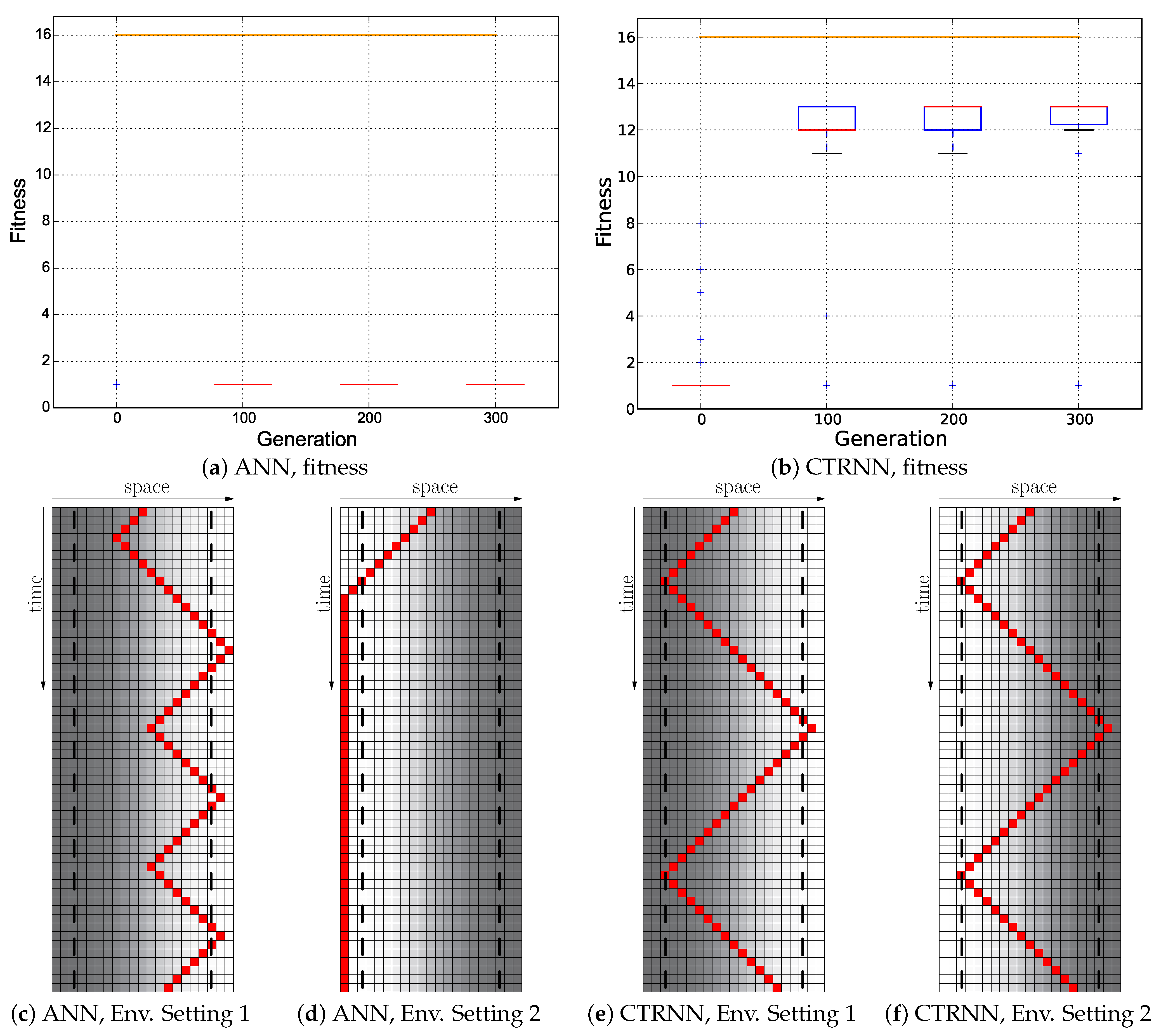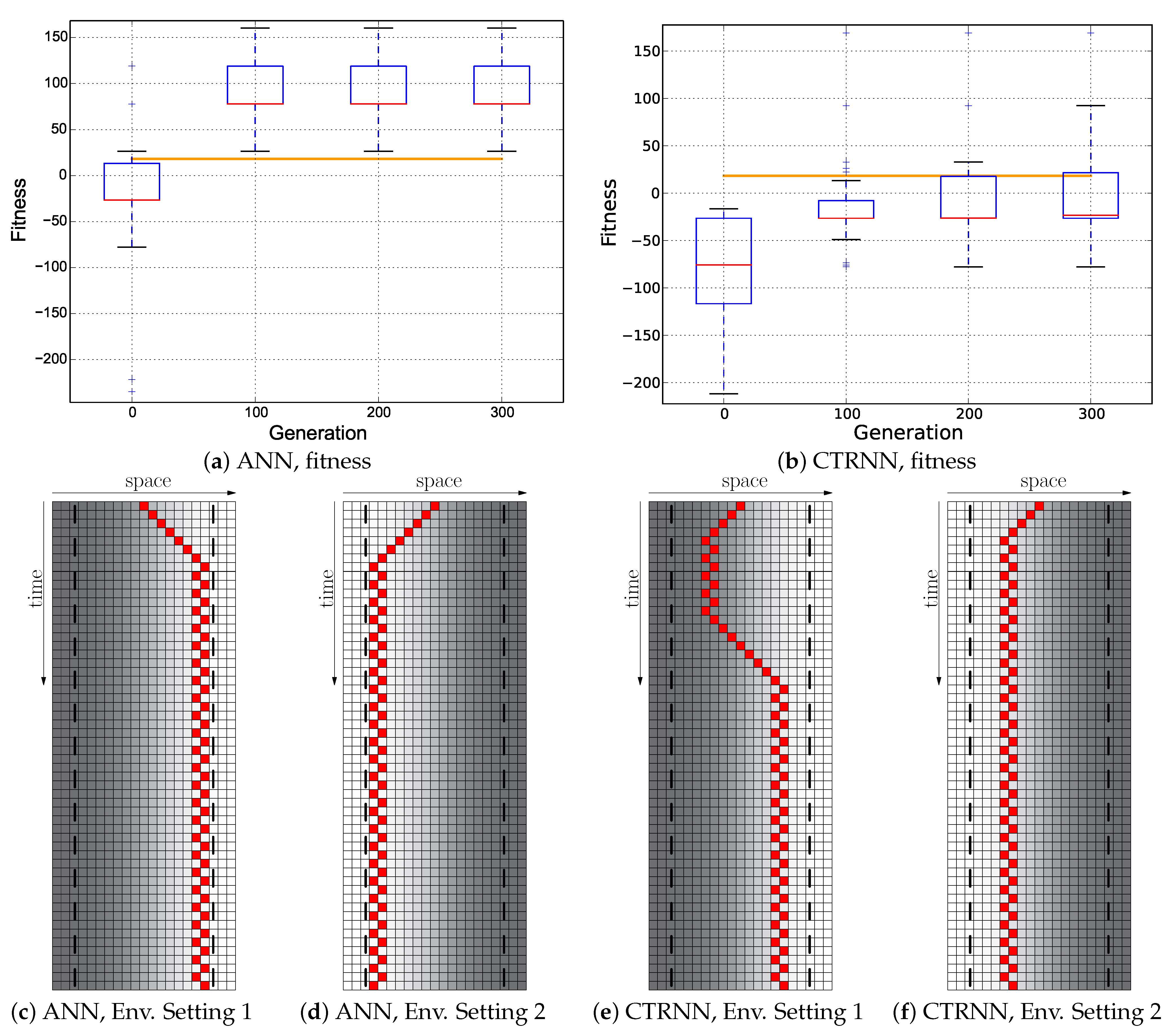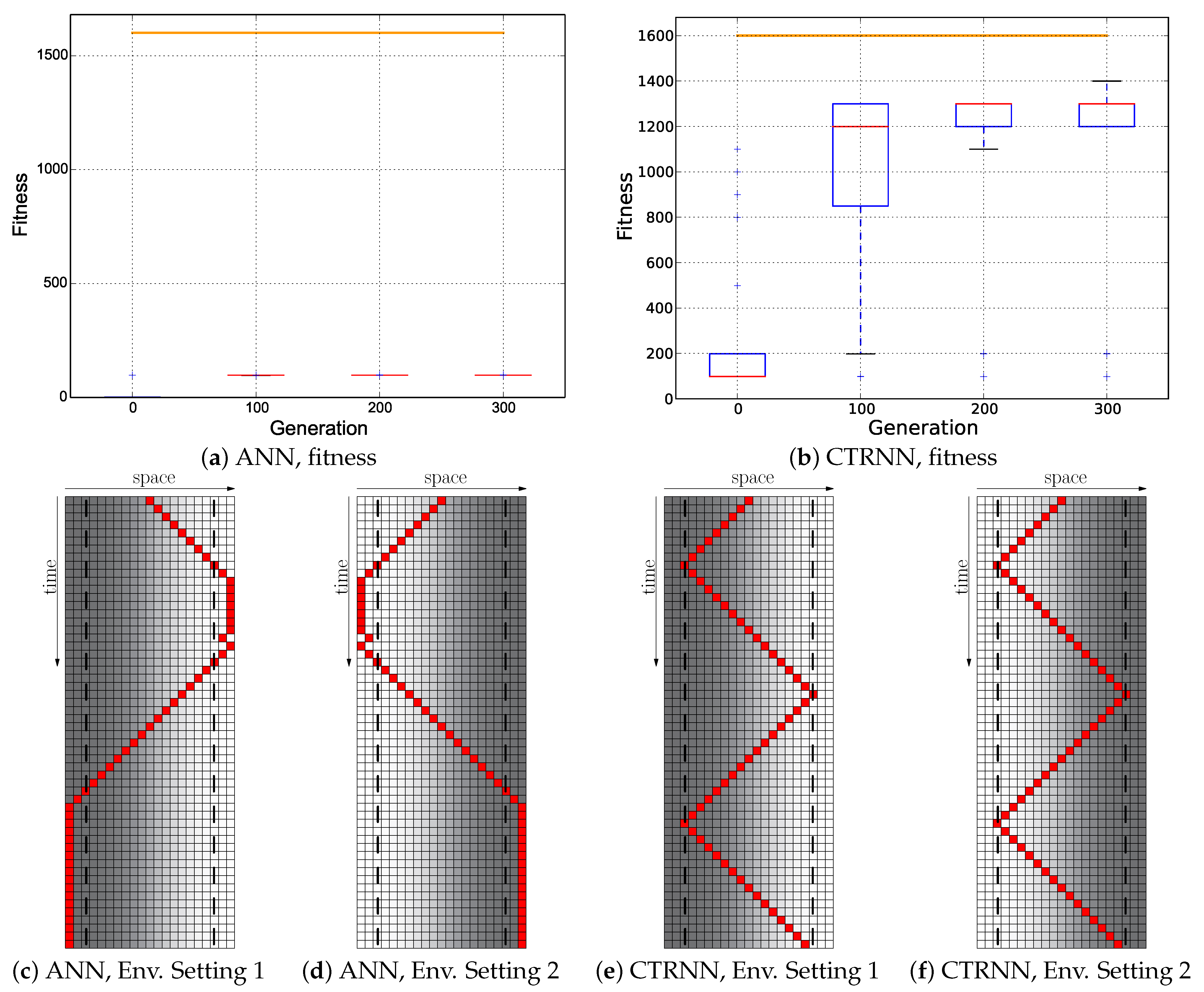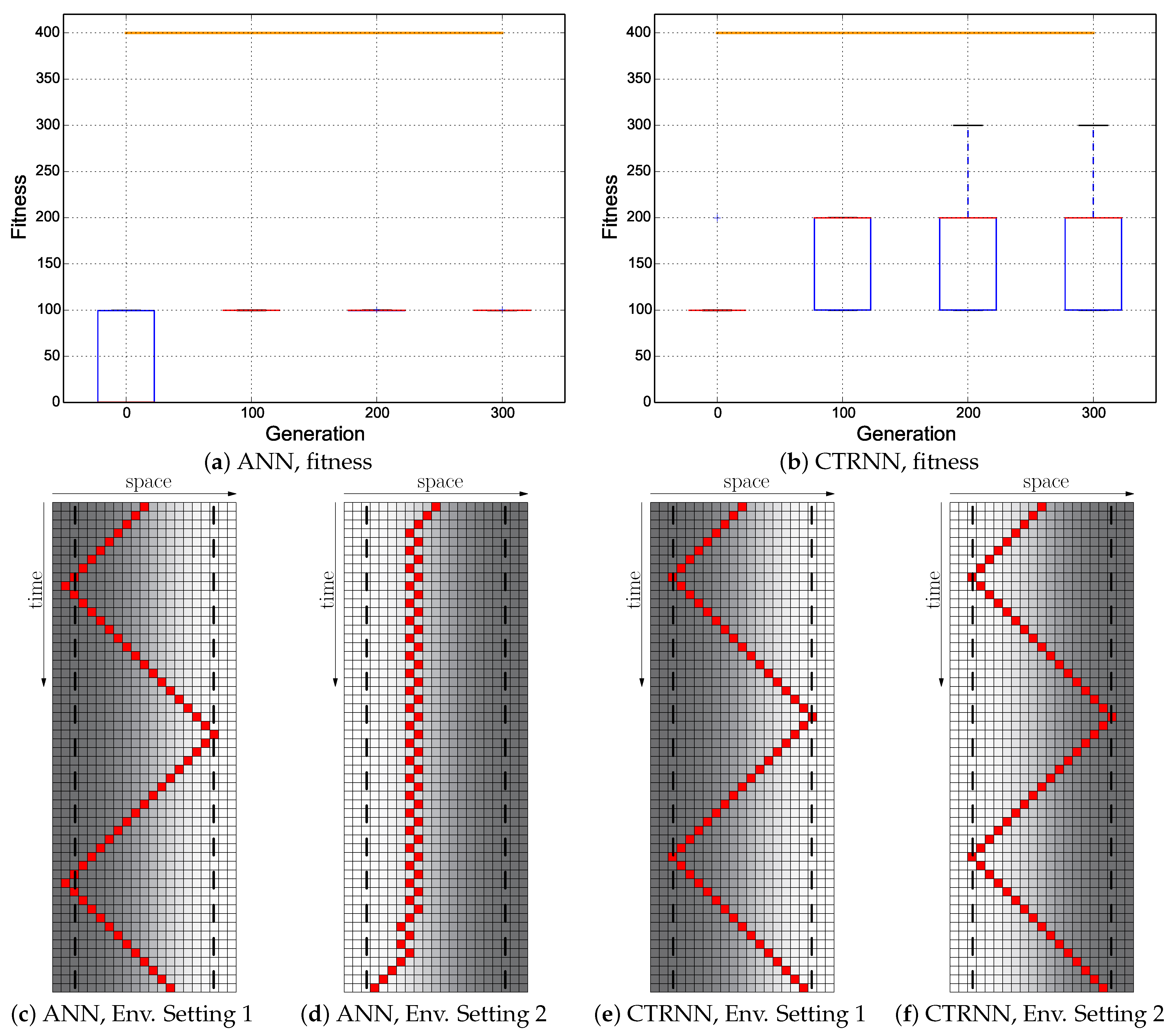Post-hoc, low-performing software controllers produced by evolutionary computation are often considered to be a consequence of bad fitness function design [7]. Therefore, we define several fitness functions and tested two software control techniques (ANN and CTRNN) using each fitness function in 30 evolutionary runs per setting, as is described in the following Quantitative Analysis Section.

5. Quantitative Analysis

5.1. Fitness Evaluation

In the experiments reported here, we used different fitness regimes based on the number of correct switches and the positioning of the agents. In order to define the different fitness regimes, three types of rewards are considered:

• Rewarding for switch: rewarding $+1$ point for every correct switch: $R_{switch}=n$, where n is the number of correct switches over the whole period of the experiment.
• Cumulative rewarding for positions: rewarding based on the state and the environmental quality of the positions of the agent accumulated over the whole period of the experiment:
  $R_{cum}={\sum }_{t=0}^{T}quality\left[P\left(t\right)\right]\times state$. That means that an agent in uphill mode ($state=1$) is rewarded the current environmental quality of its position and an agent in downhill mode ($state=-1$) is rewarded the current quality multiplied by −1. As a consequence, agents in uphill mode are rewarded positively for locating themselves in high-quality regions and agents in the downhill model for locating themselves in low-quality regions.
• Instant rewarding for final position: rewarding based on the state and the environmental quality of the final position of the agent: $R_{ins}=quality\left[P\left(T\right)\right]\times state$, where T is the period of the experiment. In this case, the reward is given for the final position of the agent. The exact value of the reward depends on the final state of the agent, but in any case, a higher reward is given if the agent is closer to the next correct switch. That means, if the agent is in the uphill mode, a higher reward is given if it is higher up the hill, and if it is in the downhill mode, a higher reward is given if it is further down the hill.

By giving different weights to the three types of rewards, the fitness function is defined as follows:

$$F(w_n,w_{cum},w_{ins})=w_{switch}\times R_{switch}+w_{cum}\times R_{cum}+w_{ins}\times R_{ins}$$

(8)

where $w_{switch}$, $w_{cum}$, and $w_{ins}$ are the parameters of the fitness function representing the weights for every type of reward.

In this study, the following fitness regimes are investigated:

• Switch:$F(1,0,0)$, rewarding only for correct switches.
• Cumulative:$F(0,1,0)$, only cumulative rewarding for positions.
• Instant + Switch: $F(100,0,0.01)$, rewarding for correct switches, as well as instant rewarding for the final position.
• Cumulative + Switch: $F(100,0.01,0)$, rewarding for correct switches, as well as cumulative rewarding for positions over the whole period.

5.2. Evolving Solutions with Non-Pre-Structured Neural Networks in Various Scenarios

In the following, we use a number of evolutionary setups (scenarios) and investigate the resulting controllers achieved by evolution in each setup. Two different controller types, ANN and CTRNN, were used. In all the scenarios, every controller ran for 250 time steps unless otherwise stated. Results were pooled from 30 independent runs for each scenario.

We used a simple genetic algorithm [25] with proportionate selection based on fitness and elitism of one. The population size was set to 150, and we ran it for 300 generations. The genome for the ANN consisted of 41 genes each encoding a connection weight between the nodes. The weights were randomly initialized between $(-0.5,0.5)$. The genome in the CTRNN consisted of 121 genes for the weights of the connections, 11 genes for the values of $\theta$, and 11 genes for the $\tau$ values of every node. The weights and $\tau$ values were randomly initialized in the range of $(-15,15)$ and $(0.9,5.9)$, respectively. The values of the $\theta$s were set based on the weights such that the richest possible dynamics was achieved, as described in [31]. We did not use a recombination operator. In the ANN, the weights were mutated with a rate of $0.3$ where a random value in $(-0.4,0.4)$ was added to the weight. In the CTRNN, the mutation rate was $0.1$ for weights and a random $\theta$ and $\tau$ were mutated at a time. The values were changed in the range of $(-0.4,0.4)$ for weights and $\theta$ and in the range of $(-0.1,0.1)$ for $\tau$.

Table 1. Parameters used for the evolutionary algorithm. CTRNN, Continuous-Time Recurrent Neural Network.

Parameter	ANN	Parameter	CTRNN
Population size	150	Population size	150
Number of genes	41	Number of genes (weights)	121
		Number of genes ($\theta$)	11
		Number of genes ($\tau$)	11
Init. range (weight)	$(-0.5,0.5)$	Init. range (weight)	$(-0.5,0.5)$
		Init. range ($\tau$)	$(0.9,5.9)$
		Init. range ($\theta$)	as in [31]
Mutation rate	0.3	Mutation rate (weights)	0.1
		Mutation rate ($\theta$, $\tau$)	randomly, one at a time

summarizes the evolutionary parameters.

5.2.1. Single Environment vs. Double Environment and Mean Fitness vs. Minimum Fitness

At first, we evaluated the performance of evolution in a fixed environment as is depicted in Figure 1. We found that evolution could quickly converge to a sort of pre-programmed trajectory (see Figure 6c,e) that achieved very high fitness (see Figure 6a,b), but was non-reactive as it did not consider sensor inputs in the wanted way. A post-hoc test of the best evolved genomes in a flipped environment, where the gradient pointed to the other side, failed for both evolved controller types, clearly indicating that no reactive Wankelmut behavior had evolved (see Figure 6d,f). The trajectories in both post-hoc runs show some difference from the runs in the environment that was used in evolution, and this indicates that some sensor input was affecting the behavior, but not in the desired way: the agents still started off in the wrong direction, and also, the oscillations ceased after some time.

As this approach did not yield the wanted reactive Wankelmut behavior, we decided to evaluate each individual genome twice: One time, the gradient pointed uphill to the left, and one time, it pointed uphill to the right side. The fitness function in all three scenarios used the Switch fitness regime, which is described as $\mathrm{fitness}=F(1,0,0)$.

We evaluated two methods of associating a fitness value with each genome from these two evaluations: first, we calculated the arithmetic mean value of both runs and, as a second variant, we took the minimum value of both runs. As a consequence, a good genome had to perform well in both environments; in the “minimum”-fitness function, the selection was even harsher than in the “mean” variant. We found that the “minimum” variant of selection showed a higher selection pressure on evolving the reactive control (compare Figure 7 and Figure 8): with the minimum fitness regime, the controllers found it harder to gather high fitness values, as they had to perform well in both environments, preventing evolution from “just considering one of the two environments”. We hoped that this would support the evolution of reactive control. As Figure 8c–f shows, it still did not produce the desired reactive Wankelmut behavior in the long run. Based on these findings, we used the double environment evaluation with a minimum-of-both-runs fitness function for all further quantitative analysis in this study, in order to maximize the selection pressure towards the reactivity of the evolved controller.

5.2.2. Cumulative Fitness Regime

In another attempt to help the evolutionary algorithm develop good reactive controllers, we decided to reward genomes purely with cumulative fitness. The idea behind this was that every single step in the correct direction would be paying off in evolution. We assumed that, on the one hand, bootstrapping problems of achieving early success during evolution were minimized in this way. On the other hand, early developments of appropriate, reactive turns of agents were rewarded even if they did not yet occur at the correct positions according to an appropriate switching threshold. In this scenario, the fitness was computed by the Cumulative fitness regime described as $\mathrm{fitness}=F(0,1,0)$.

We found that the idea of cumulative fitness for every step was exceptionally bad. To our surprise, both controller types managed to even significantly outperform the hand-coded “optimal” controller (see Figure 9a,b). Looking at the trajectories revealed that the evolutionary algorithm had found the NAUSS to maximize this purely cumulative fitness function without evolving the desired task: the controllers approached the threshold areas, thus gained the maximum reward without having to switch the behavior. They kept this place for the rest of the run. Such undesired solutions were found by the evolutionary process with both controller types, with the ANNs (see Figure 9c,d) and also with CTRNNs (see Figure 9e,f) in a less effective way. In both cases, the agent actively avoided behaving similar to the desired reactive Wankelmut controller by avoiding crossing the threshold places. This way of maximizing the fitness function without improving the agent’s behavioral quality is clearly a shortcoming in the fitness function design that resulted in the evolutionary algorithm getting stuck in the local optimum by gaining rewards for a behavior that does not allow further complexification towards the desired final behavioral program.

5.2.3. Instant + Switch Fitness Regime

In order to prevent the evolutionary computation from getting stuck due to being able to exploit the NAUSS we discovered in the previous section, we again revised our fitness function to the Instant + Switch reward setting: We again rewarded for every correct switch the agent performed, and instead of a cumulative reward every time step, we rewarded the final (one instant) position of the agent. This way, bootstrapping problems could also be mediated as again movement in the right direction without reaching the threshold place for switching the behavior would be rewarded, but it did not pay out to keep the position just before triggering the switch. The fitness function used here can be described as $\mathrm{fitness}=F(100,0,0.01)$.

The highest fitness values in this setting were achieved by the CTRNNs (see Figure 10b). However, this was again achieved by just quickly zig-zagging across the world without adaptively reacting to the environmental situation: the agents started off in the wrong direction (see Figure 10e,f) in one environmental setting. Evolved ANNs did not at all develop highly rewarded behaviors in this setting (see Figure 10a). However, the best ANN genome evolved in principle parts of the desired behaviors for the first period of time: they started off in both environments in the correct direction and executed the behavioral switch one time, but never closed the cycle back again (see Figure 10c,d). Overall, the desired reactive Wankelmut behavior was never fully evolved in either one of the controller types.

5.2.4. Cumulative + Switch Fitness Regime

In a final attempt to achieve the desired behavior, we also tested the Cumulative + Switch fitness regime where the controller was rewarded cumulatively for positioning of the agent over time, as well as significant rewards for the correct switches were given. The fitness function can be described as $\mathrm{fitness}=F(100,0.01,0)$.

Introducing the additional rewarding for correct switches prevented the evolutionary algorithm from falling into local optima (NAUSS) as it did when it was only rewarded cumulatively per step. The results were almost similar to the ones obtained from the previous Instant + Switch regime: the CTRNNs did not evolve anything close to the desired reactive Wankelmut behavior (see Figure 11), and the ANNs evolved again the first switching of behaviors, but failed to evolve the switch back (see Figure 11c,d). The CTRNNs achieved again a significant reward by oscillating in both environments in a non-reactive oscillatory behavior (see Figure 11e,f), like they evolved already in most of the other evolution regimes.

In another attempt to enforce the reactivity of the evolved controller and considering the evolved solutions shown above, we tried to push the evolution towards more reactivity of the controllers. Thus, the evolutionary experiment was repeated with only 56 time steps per evaluation (see Figure 12). Again, the CTRNNs evolved a higher fitness (Figure 12b) than the ANNs (Figure 12a). However, this was still achieved with non-reactive fast oscillations (see Figure 12e,f). The ANNs evolved into a behavior that oscillated in one environment although starting in the wrong direction initially (see Figure 12c. In the second environment, the best agent progressed very slowly towards the threshold place, and no switch back was observed there Figure 12d).

The resulting controllers were also tested in a post-evaluation to check for reactive behaviors. This was done with a different environment that had maximum quality in the middle and two minima, one at the left end and one at the right end. Agents were tested in two evaluations with one initially positioning the robot at the left end and the second one with initially positioning the robot at the right end. While some controllers managed to operate reasonably in one of the two evaluations (oscillating between the initial position and the middle place), none of them did so for both starting places. Hence, we concluded that also in this experiment, we did not see the correct controller that solved the Wankelmut task in a reactive way.

5.3. Evolving a Pre-Structured Hand-Coded Network

One of the hand-coded ANNs along with its behavior in the two environments is represented in Figure 5a–c. Although the agent is reactive and switches after passing the thresholds on each side, the behavior is not optimal. The agent exhibits a delay in switching when it passes the thresholds in the environment represented in Figure 5c. In an attempt to get closer to the known perfect behavior, we initialized an ANN described in Section 4.1 with the weights of a hand-coded ANN and then used each of the described fitness functions to further evolve the network. We performed this form of post-hoc evolution process with all four fitness functions described above. When using the Switch fitness function, the evolutionary process developed an ANN that showed near-optimal adaptive behavior (see Figure 13), as it was also found to evolve when using both the Cumulative + Switch fitness function (Figure 14) and the Instant + Switch fitness function (Figure 15). However, when applying the Cumulative fitness function, an ANN evolved with a non-reactive and non-adaptive NAUSS behavior (Figure 16). Figure 5d–f shows the best evolved network, including the weights, as well as the behaviors of the agent that was governed by this network and its set of weights in both tested environments. As seen in these figures, the evolutionary process flattened the ANN by adding values to additional links between nodes and layers. As a consequence, this evolved ANN demonstrated the optimal behavior.

5.4. Summarizing Our Experimental Results

In total, we studied 20 different evolutionary settings with different combinations of the computational substrate that the evolutionary process could shape, of the used fitness function, and of the agent’s environment. Figure 3 shows the results of the different experimental tracks and their final outcomes.

6. Discussion and Conclusions

We propose the Wankelmut task, which is a very simple task. Compared to the classification scheme of Braitenberg [24], an agent that solves the Wankelmut task would be placed between Vehicle #4 and Vehicle #5 concerning the complexity of its behavior. Given that it operates in a one-dimensional space introduces a relation to Vehicle #1. In the Wankelmut task, we evolve a controller that switches between two alternative conflicting tasks. Yet, there is no prioritizing between the two subtasks, and therefore, it is not a subsumption architecture. It also does not repeatedly alternate between two subtasks since the switching between the two tasks is based on the environmental clues. The simplicity of the pseudo-code shown in Figure 2 clearly demonstrates the simplicity of the required controller that implements an optimal, flexible, and reactive Wankelmut agent.

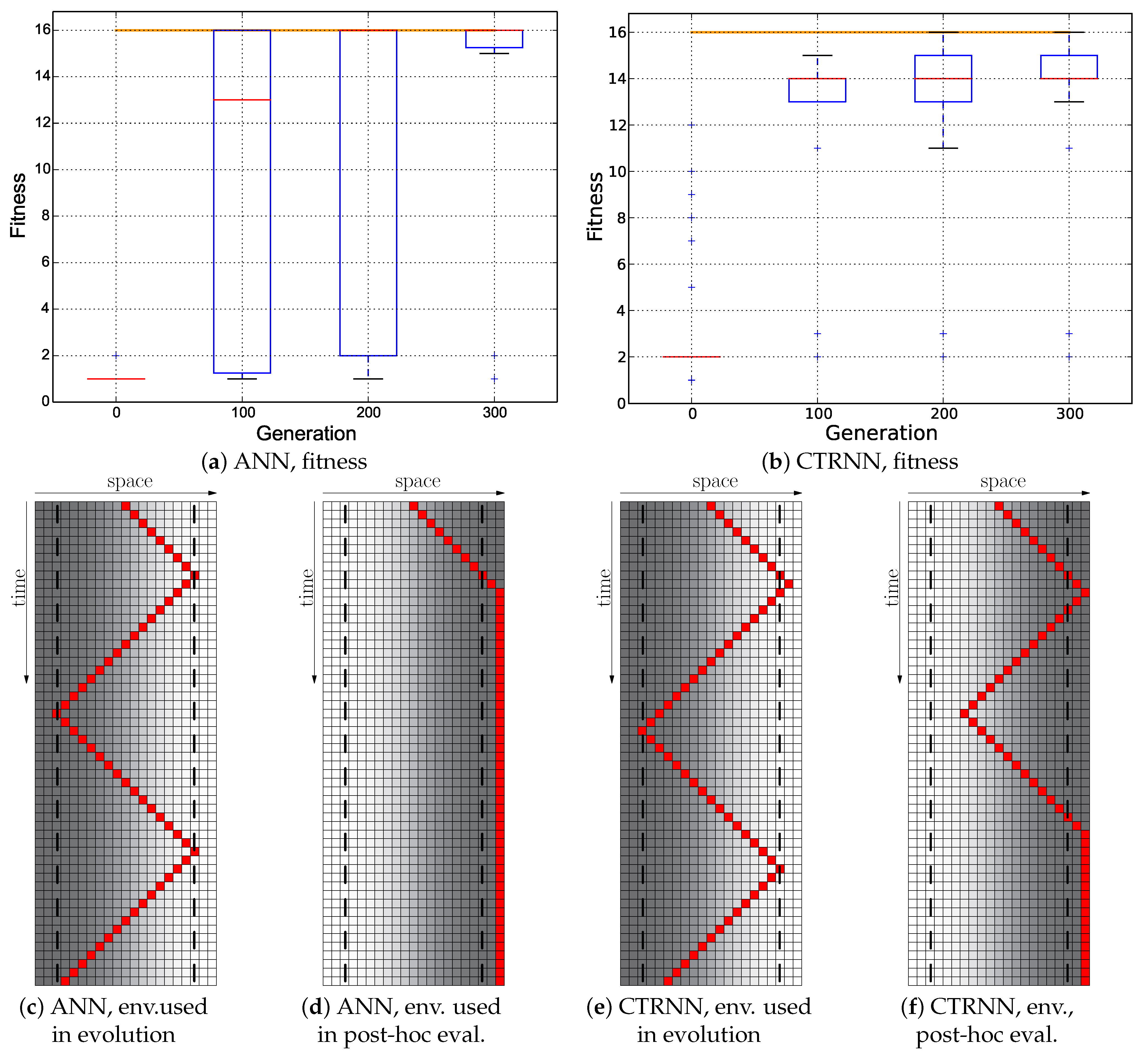
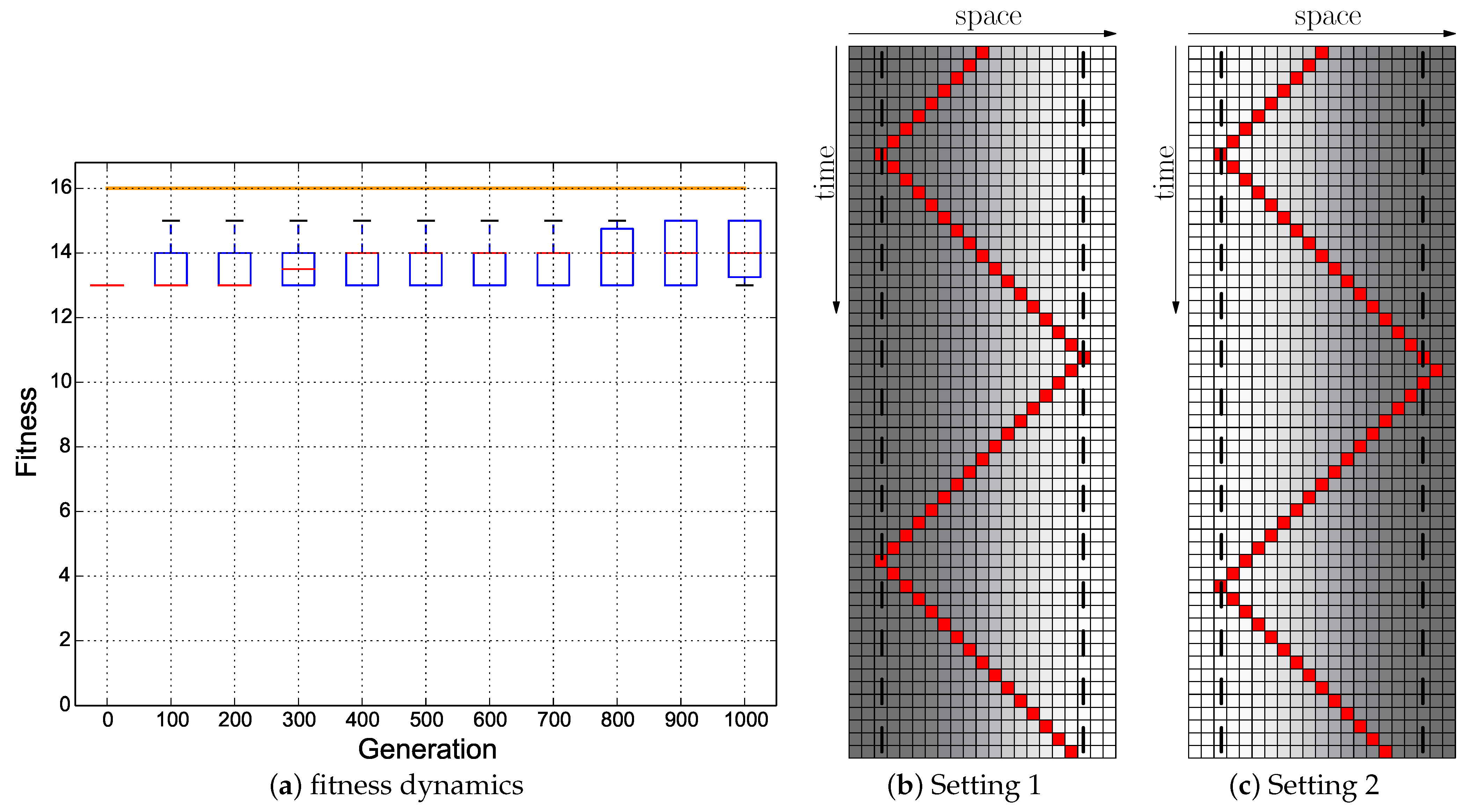
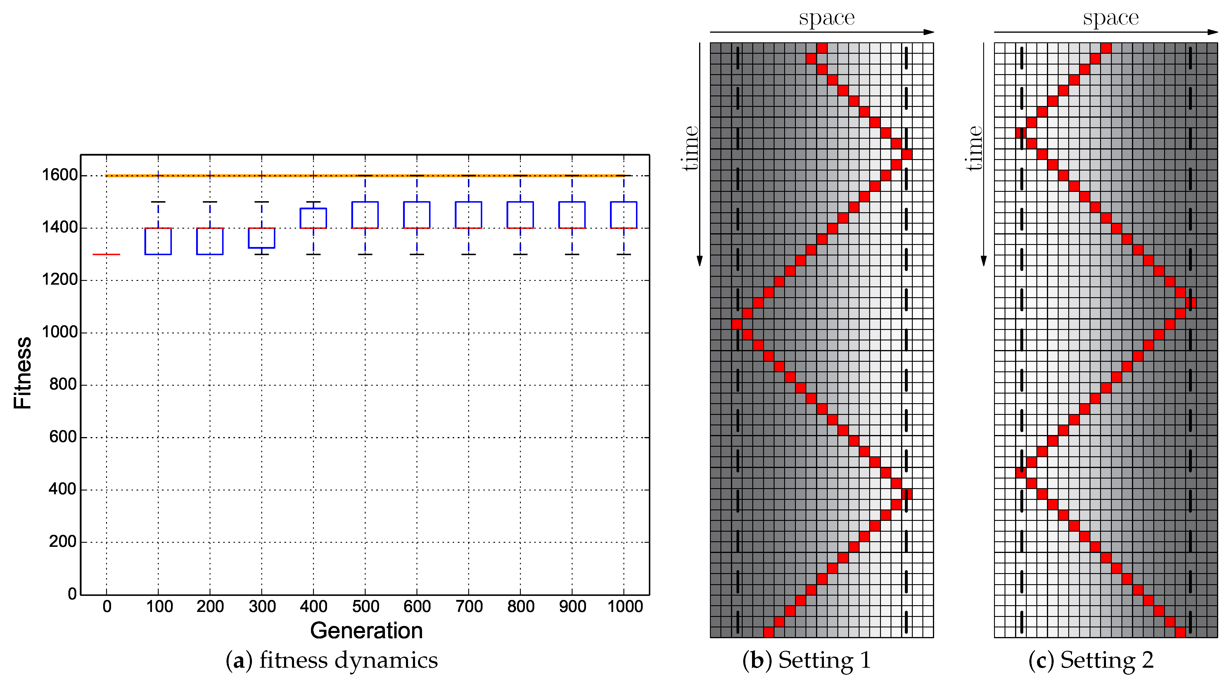
Our results indicate that plain-vanilla evolving ANNs easily can evolve the reactive uphill walk (see Figure 6c). However, switching to the opposite behavior (downhill motion) and then flipping back was not found by any of our approaches, regardless of what fitness regime we used and regardless of which neuronal architecture we used as a substrate for the evolutionary process (ANN or CTRNN). In all tested fitness regimes, the desired behavior did not evolve. 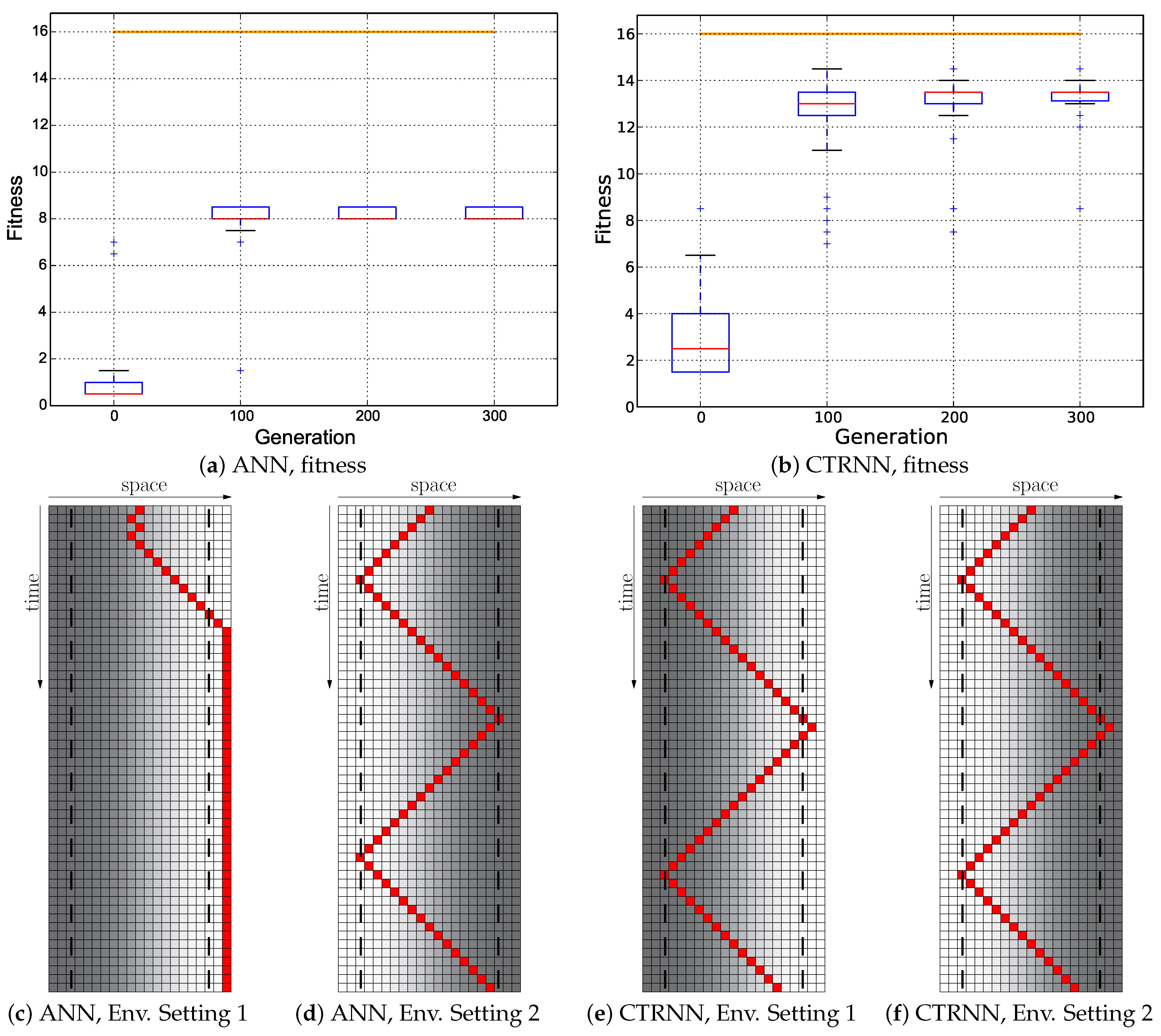In one of these fitness regimes (Cumulative regime), evolution found a “heap trick” to maximize the fitness with a surprising behavior; however, the desired reactive Wankelmut behavior did not evolve there.

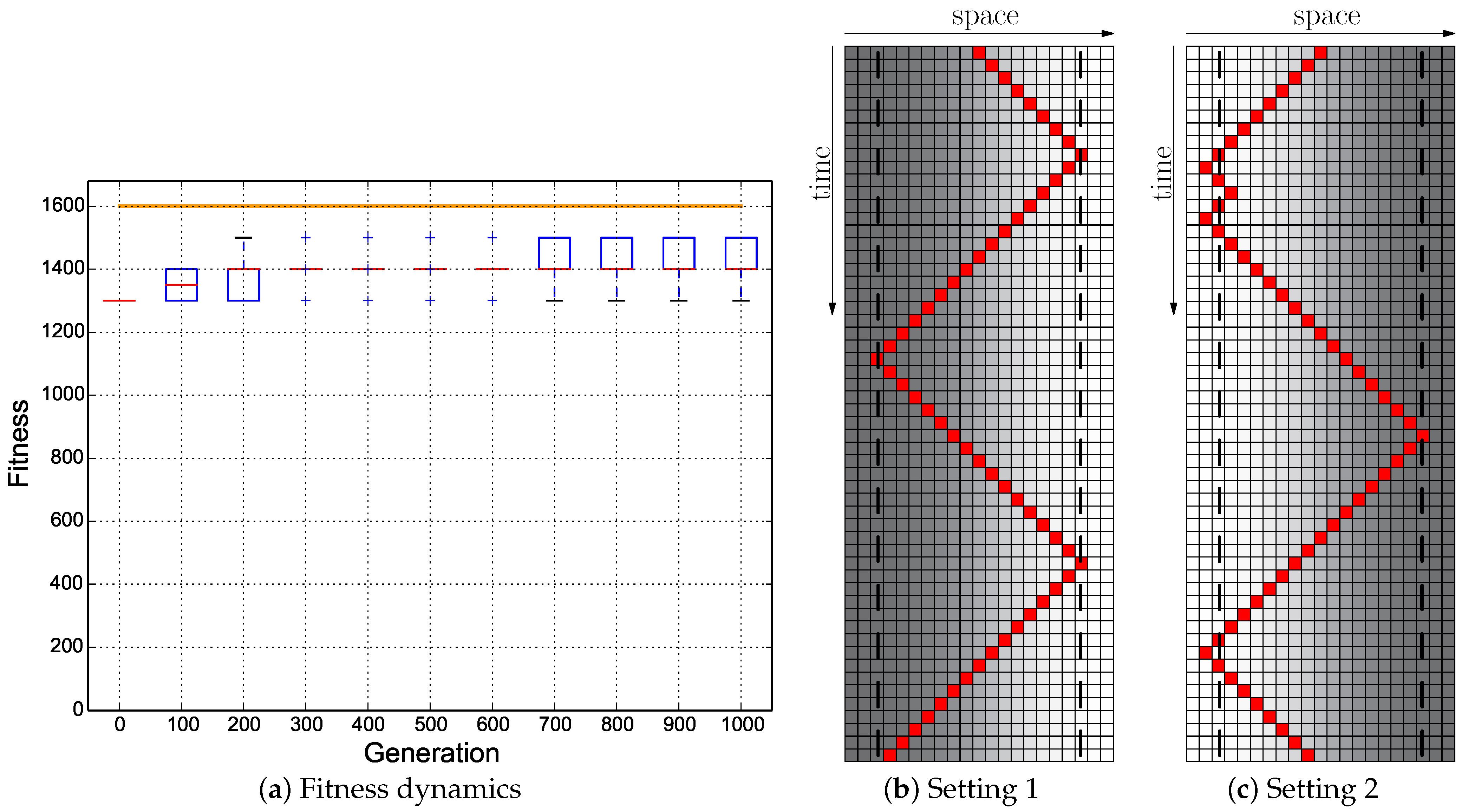
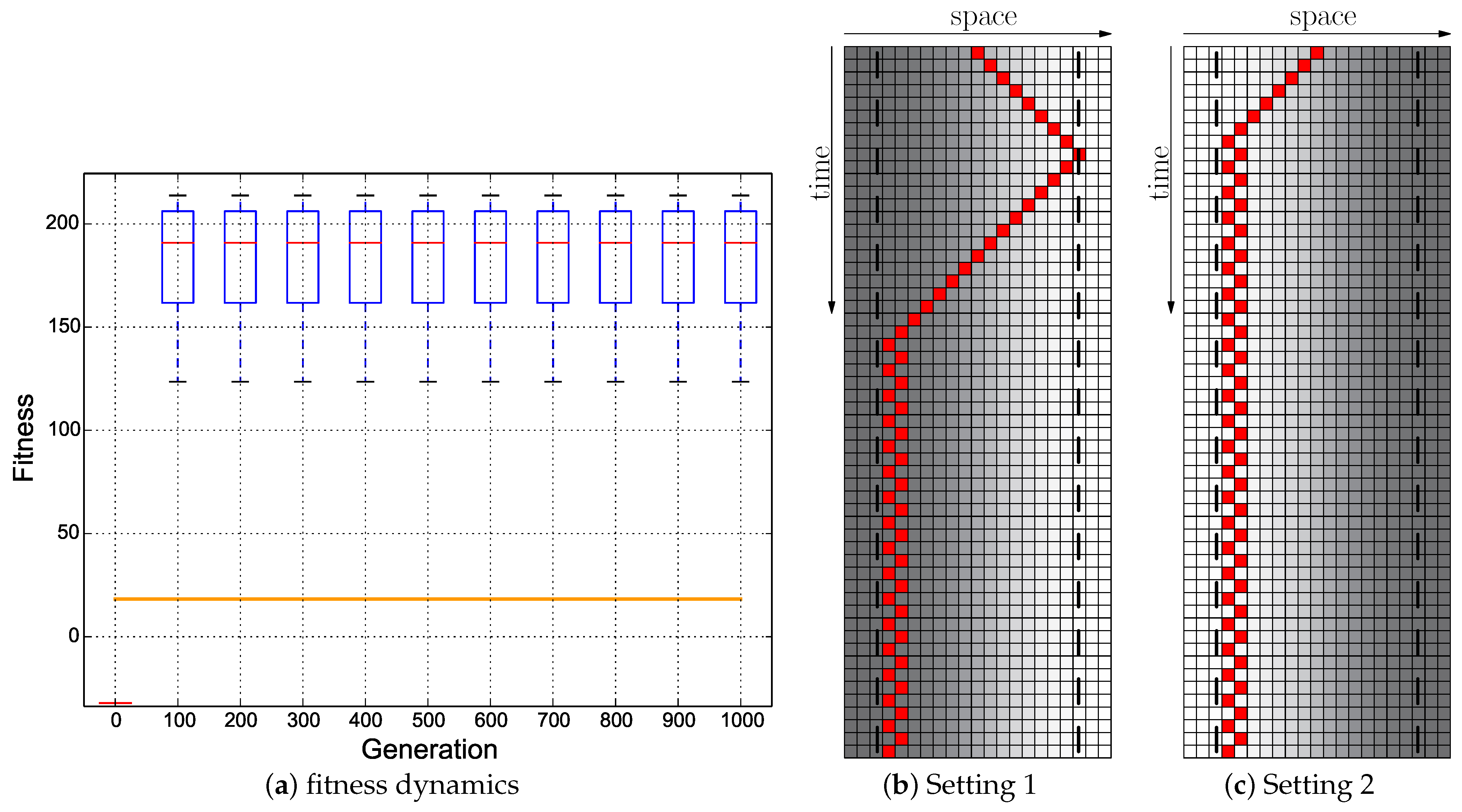
In order to prove that the task is solvable by the encoding that we used here, we designed two hand-coded ANNs to solve the task. However, the hand-coded networks demonstrated a behavior that was quite good, but not optimal. To further improve this, we then evolved one of the hand-coded ANNs and achieved the optimal behavior showing that the encoding covers the solution and the evolution can evolve the behavior when it is searching in the vicinity of the solution (Figure 5).

In summary, Wankelmut is an easy-to-implement benchmark task that can be solved by two simple hand-coded lines of code (see Figure 2). Despite its simplicity, it was found to be a hard task for evolutionary algorithms to solve, as all our evolutionary trajectories without access to a priori information about how to solve the task failed to achieve the desired adaptive behaviors. To investigate the role of modularity in this process, we created pre-structured neural networks, where the weights were initialized to provide an appropriate adaptive, but still suboptimal solution, and allowed to be optimized by the evolutionary process, as shown in Figure 3. These experiments yielded sub-optimal, but reactive behavioral controllers that produced a correct Wankelmut-like behavior, thus indicating a step forward concerning evolvability. By further hand-tuning of these evolved networks, we were able to implement an improvement that resulted in optimal adaptive behaviors, demonstrating that the offered computational substrate was capable of producing the desired behavior.

When looking at Figure 3, it becomes clear that only the hand-coded controller depicted in Figure 2 showed the desired Wankelmut behavior, as did also the hand-coded and pre-structured ANNs in an almost similar way. From all evolutionary runs that we performed, only those showed a close-to-optimal Wankelmut behavior that started the evolutionary process already with a pre-structured network and that then evolved this structure further with an appropriate fitness function (Switch, Instant + Switch, or Cumulative + Switch).This stresses, on the one hand, the simplicity of computational structures that are required to fulfill the task and the need of having the evolutionary computation already informed about the path towards the solution, which is a structure consisting of three interconnected modules: two for each of the antagonistic behaviors and one as a higher order regulatory element that negotiates between those two other modules.

Based on these observations, we come to the interpretation that a pre-defined suitable modularity of the network helps, but is not sufficient for optimal results. A method to achieve optimal results needs to either have the required modules available from the beginning and then ensure that this modularity is used beneficially in the evolutionary process or, even more desired, be able to create the needed modularity during the evolutionary process by itself. We designed the Wankelmut task on purpose to consist of two opposing behaviors (uphill and downhill walk) that cannot be performed at the same time in order to generate a hard-to-learn task. Neural structures that are beneficial to create downhill behavior cannot be easily converted into structures that produce uphill behavior without “destroying” the previously learned network functionality, if there is no other higher level of control preventing it (cf. catastrophic forgetting [34]). Thus, in order to evolve a combination of both, it would require a specific evolutionary framework that is designed to generate functional modules, to store (freeze) useful modules and then to combine them with more complex behaviors like the Wankelmut task. However, such a functionality was not found to evolve from scratch by itself in our system in an emergent way.

Given that the hand-coded solution is simple, a tree-based approach with exhaustive search or a Genetic Programming (GP) approach [35] is expected to be able to find the desired behavior. However, we would expect also here to hit the same “wall of complexity”, as controllers that require a bit more complexity overwhelm the exhaustive tree-search, while the existing local optima, that already fooled the ANN + Evoapproach and the CTRNN + Evo approach, will also fool the stochastic GP search in a similar way. This remains to be tested in future experiments.

We point out that the target of evolving controllers for the Wankelmut task from scratch requires evolving a behavioral switch. However, the evolution of such a switch represents a chicken-egg problem. The switch is useless without the two motion modules (subnets) for uphill and downhill motion, while those sub-modules are useless without the switch.

In addition, we want to point out the fact that a similar behavior could be exerted by just switching the environment in an oscillatory way. This is not the same as our envisioned Wankelmut behavior, as our behavior intrinsically switches its behavioral pattern in reaction to a stable environment. Therefore, it is intrinsic dynamics exhibited in a global stable environment and not a fixed (stable) behavioral pattern in a globally dynamic environment.

The Wankelmut task might also prove to be an interesting benchmark for more sophisticated methods that push towards modularization. Examples are artificial epigenetic networks as reported by Turner et al. [36]: they used the coupled inverted pendulums benchmark [37], which requires the concurrent evolution of several behaviors similar to the Wankelmut task. However, the control of coupled inverted pendulums is more complex than the simple world of Wankelmut. Other methods alternate between different tasks on evolutionary time-scales [21], and there are methods that, in addition, also impose costs on connections between nodes in neural networks [22]. Other interesting approaches either pre-determine or push towards modularity [18]. The approach of HyperNEAT was tested for its capability to generate modular networks with a negative result in the sense that modularity was not automatically generated [38]. Bongard [39] reported modularity by imposing different selection pressures on different parts of the network.

In fact, we propose here two challenges for the scientific community at once:

• The first challenge is to find the most simple uninformed evolutionary computation algorithm that can solve the Wankelmut task presented here. Then, the community can search for the next simple task that is shown to be unsolvable for this new algorithm. This will yield iterative progress in the field.
• The Wankelmut task is the simplest task found so far (concerning required memory size, number of modules, dimensionality of the world it operates in, etc.). Still, there might be even simpler tasks that already break plain-vanilla uninformed evolutionary computation, so we also pose the challenge to search for such simpler benchmark tasks.

It should be noted that there is no evidence that such walls of complexity are consistent in a way that breaking one wall may cause a new wall at a different position. This is quite similar to the reasoning behind the “no free lunch” theorem. Theoretically, an optimization algorithm cannot be optimal for all tasks. However, neither natural nor artificial evolution achieve in general optimal solutions. Instead, especially natural evolution has proven to be a great heuristic for which the walls might be fixed in a certain place but, definitely far away from the wall for state-of-the-art artificial evolution. Hence, we should try to search for that one heuristic that allows us to push all walls of many different tasks as far as possible forward (while still accepting the implications of no free lunch).

We think that either dismissing all pre-informed methods or finding minimally pre-informed methods to solve the Wankelmut task is important. Natural evolution has produced billions of billions of reactive and adaptive behaviors of organisms much more complex than the Wankelmut task, and it has achieved this without any information that promoted self-complexification and self-modularization. In contrast, the evolutionary process started from scratch and developed all of that due to evolution-intrinsic forces. We think that this can be a lesson for evolutionary computation: studying how an uninformed process that is neither pre-fabricated towards complexification or modularization and that is not specifically rewarded for complexification or modularization can still yield complex solutions. Nature has shown this, and evolutionary computation and biologists together should find out how this was achieved. Perhaps, this would then not be “evolutionary computation’ anymore, but rather “artificial evolution”, a real valid, yet still simple model of natural evolution. This might be achieved by incorporating the principles of biological growth, for example the mechanisms of Evolutionary Developmental biology, “EvoDevo” [40], which might be the path to evolve future in silico neuromorphic computation systems [41] and virtual brains [42] via embryogenetic or morphogenetic algorithms [43] that can develop the required capabilities of self-modularization and self-complexification, in order to break through the walls of complexity that we discovered.

References

1. Sutton, R.S.; Barto, A.G. Reinforcement Learning: An Introduction; MIT Press: Cambridge, MA, USA, 1998. [Google Scholar]
2. Bongard, J.C. Evolutionary robotics. Commun. ACM 2013, 56, 74–83. [Google Scholar] [CrossRef] [Green Version]
3. Prokopenko, M. Grand challenges for Computational Intelligence. Front. Robot. AI 2014, 1. [Google Scholar] [CrossRef] [Green Version]
4. Eiben, A.E.; Smith, J. From evolutionary computation to the evolution of things. Nature 2015, 521, 476–482. [Google Scholar] [CrossRef] [PubMed]
5. Jakobi, N.; Husbands, P.; Harvey, I. Noise and the Reality Gap: The Use of Simulation in Evolutionary Robotics. In Proceedings of the Third European Conference on Advances in Artificial Life; Springer: Berlin/Heidelberg, Germany, 1995; Volume 929, pp. 704–720. [Google Scholar]
6. Nolfi, S.; Floreano, D. Evolutionary Robotics: The Biology, Intelligence, and Technology of Self-Organizing Machines; MIT Press: Cambridge, MA, USA, 2000. [Google Scholar]
7. Nelson, A.L.; Barlow, G.J.; Doitsidis, L. Fitness functions in evolutionary robotics: A survey and analysis. Robot. Auton. Syst. 2009, 57, 345–370. [Google Scholar] [CrossRef]
8. Silva, F.; Duarte, M.; Correia, L.; Oliveira, S.M.; Christensen, A.L. Open Issues in Evolutionary Robotics. Evol. Comput. 2016, 24, 205–236. [Google Scholar] [CrossRef] [PubMed]
9. Wolpert, D.H.; Macready, W.G. No free lunch theorems for optimization. Evol. Comput. IEEE Trans. 1997, 1, 67–82. [Google Scholar] [CrossRef] [Green Version]
10. Marocco, D.; Nolfi, S. Origins of Communication in Evolving Robots. In From Animals to Animats 9: Proceedings of the Eighth International Conference on Simulation of Adaptive Behavior; LNCS; Springer: Berlin/Heidelberg, Germany, 2006; Volume 4095, pp. 789–803. [Google Scholar]
11. Sims, K. Evolving 3D Morphology and Behavior by Competition. In Artificial Life IV; Brooks, R., Maes, P., Eds.; MIT Press: Cambridge, MA, USA, 1994; pp. 28–39. [Google Scholar]
12. Clune, J.; Beckmann, B.E.; Ofria, C.; Pennock, R.T. Evolving Coordinated Quadruped Gaits with the HyperNEAT Generative Encoding. In Proceedings of the 2009 IEEE Congress on Evolutionary Computation (CEC), Trondheim, Norway, 18–21 May 2009; pp. 2764–2771. [Google Scholar]
13. Zahadat, P.; Christensen, D.; Katebi, S.; Stoy, K. Sensor-coupled Fractal Gene Regulatory Networks for Locomotion Control of a Modular Snake Robot. In Distributed Autonomous Robotic Systems; Springer: Berlin/Heidelberg, Germany, 2010; pp. 517–530. [Google Scholar]
14. Hamann, H.; Stradner, J.; Schmickl, T.; Crailsheim, K. A Hormone-Based Controller for Evolutionary Multi-Modular Robotics: From Single Modules to Gait Learning. In Proceedings of the IEEE Congress on Evolutionary Computation (CEC’10), Barcelona, Spain, 18–23 July 2010; pp. 244–251. [Google Scholar]
15. Zahadat, P.; Schmickl, T.; Crailsheim, K. Evolving Reactive Controller for a Modular Robot: Benefits of the Property of State-Switching in Fractal Gene Regulatory Networks. In From Animals to Animats 12; Lecture Notes in Computer Science; Ziemke, T., Balkenius, C., Hallam, J., Eds.; Springer: Berlin/Heidelberg, Germany, 2012; Volume 7426, pp. 209–218. [Google Scholar] [CrossRef] [Green Version]
16. Floreano, D.; Keller, L. Evolution of Adaptive Behaviour in Robots by Means of Darwinian Selection. PLoS Biol. 2010, 8, e1000292. [Google Scholar] [CrossRef] [PubMed] [Green Version]
17. Lipson, H. Principles of modularity, regularity, and hierarchy for scalable systems. In Proceedings of the GECCO Workshop on Modularity, Regularity, and Hierarchy in Evolutionary Computation, Seattle, WA, USA, 26–30 June 2004; pp. 125–128. [Google Scholar]
18. Nolfi, S. Using Emergent Modularity to Develop Control Systems for Mobile Robots. Adapt. Behav. 1996, 5, 343–363. [Google Scholar] [CrossRef] [Green Version]
19. Urzelai, J.; Floreano, D.; Dorigo, M.; Colombetti, M. Incremental Robot Shaping. Connect. Sci. 1998, 10, 341–360. [Google Scholar] [CrossRef] [Green Version]
20. Duro, R.J.; Becerra, J.A.; Santos, J. Behavior reuse and virtual sensors in the evolution of complex behavior architectures. Theory Biosci. 2001, 120, 188–206. [Google Scholar] [CrossRef]
21. Kashtan, N.; Alon, U. Spontaneous evolution of modularity and network motifs. Proc. Natl. Acad. Sci. USA 2005, 102, 13773–13778. [Google Scholar] [CrossRef] [PubMed] [Green Version]
22. Clune, J.; Mouret, J.B.; Lipson, H. The evolutionary origins of modularity. Proc. R. Soc. B 2013, 280, 20122863. [Google Scholar] [CrossRef] [PubMed] [Green Version]
23. Shallice, T. From Neuropsychology to Mental Structure; Cambridge University Press: Cambridge, UK, 1988. [Google Scholar]
24. Braitenberg, V. Vehicles: Experiments in Synthetic Psychology; MIT Press: Cambridge, MA, USA, 1984. [Google Scholar]
25. Holland, J.H. Adaptation in Natural and Artificial Systems; Univ. Michigan Press: Ann Arbor, MI, USA, 1975. [Google Scholar]
26. Rechenberg, I. Evolutionsstrategie. Optimierung Technischer Systeme nach Prinzipien der Biologischen Evolution; Frommann Holzboog: Stuttgart, Germany, 1973. [Google Scholar]
27. Darwin, C. On the Origin of Species by Means of Natural Selection; John Murray: London, UK, 1859. [Google Scholar]
28. Seeley, T.D. The Wisdom of the Hive: The Social Physiology of Honey Bee Colonies; Havard University Press: Cambridge, MA, USA; London, UK, 1995. [Google Scholar]
29. Camazine, S.; Deneubourg, J.L.; Franks, N.R.; Sneyd, J.; Theraulaz, G.; Bonabeau, E. Self-Organizing Biological Systems; Princeton Univ. Press: Princeton, NJ, USA, 2001. [Google Scholar]
30. Funahashi, K.I.; Nakamura, Y. Approximation of dynamical systems by continuous time recurrent neural networks. Neural Netw. 1993, 6, 801–806. [Google Scholar] [CrossRef]
31. Beer, R.D. Parameter space structure of continuous-time recurrent neural networks. Neural Comput. 2006, 18, 3009–3051. [Google Scholar] [CrossRef] [PubMed]
32. Lehman, J.; Clune, J.; Misevic, D.; Adami, C.; Altenberg, L.; Beaulieu, J.; Bentley, P.J.; Bernard, S.; Beslon, G.; Bryson, D.M.; et al. The Surprising Creativity of Digital Evolution: A Collection of Anecdotes from the Evolutionary Computation and Artificial Life Research Communities. arXiv 2019, arXiv:1803.03453. [Google Scholar] [CrossRef] [PubMed] [Green Version]
33. Koos, S.; Mouret, J.B.; Doncieux, S. Crossing the Reality Gap in Evolutionary Robotics by Promoting Transferable Controllers. In Proceedings of the 12th Annual Conference on Genetic and Evolutionary Computation, GECCO ’10, Portland, OR, USA, 7–11 July 2010; Association for Computing Machinery: New York, NY, USA, 2010; pp. 119–126. [Google Scholar] [CrossRef] [Green Version]
34. French, R.M. Catastrophic forgetting in connectionist networks. Trends Cogn. Sci. 1999, 3, 128–135. [Google Scholar] [CrossRef]
35. Koza, J.R. Genetic Programming: On the Programming of Computers by Means of Natural Selection; MIT Press: Cambridge, MA, USA, 1992. [Google Scholar]
36. Turner, A.P.; Caves, L.S.D.; Stepney, S.; Tyrrell, A.M.; Lones, M.A. Artificial Epigenetic Networks: Automatic Decomposition of Dynamical Control Tasks Using Topological Self-Modification. IEEE Trans. Neural Networks Learn. Syst. 2016. [Google Scholar] [CrossRef] [PubMed] [Green Version]
37. Hamann, H.; Schmickl, T.; Crailsheim, K. Coupled inverted pendulums: A benchmark for evolving decentral controllers in modular robotics. In Proceedings of the 13th Annual Genetic and Evolutionary Computation Conference, GECCO 2011, Dublin, Ireland, 12–16 July 2011; Krasnogor, N., Lanzi, P.L., Eds.; ACM: New York, NY, USA, 2011; pp. 195–202. [Google Scholar]
38. Clune, J.; Beckmann, B.E.; McKinley, P.K.; Ofria, C. Investigating whether hyperNEAT produces modular neural networks. In Proceedings of the 12th Annual Conference on Genetic and Evolutionary Computation, Portland, OR, USA, 7–11 July 2010; pp. 635–642. [Google Scholar]
39. Bongard, J.C. Spontaneous evolution of structural modularity in robot neural network controllers: Artificial life/robotics/evolvable hardware. In Proceedings of the 13th Annual Conference on Genetic and Evolutionary Computation, GECCO ’11, Dublin, Ireland, 12–16 July 2011; ACM: New York, NY, USA, 2011; pp. 251–258. [Google Scholar]
40. Carroll, S.B. Endless Forms Most Beautiful: The New Science of Evo Devo and the Making of the Animal Kingdom; Number 54; WW Norton & Company: New York, NY, USA, 2005. [Google Scholar]
41. Esser, S.K.; Merolla, P.A.; Arthur, J.V.; Cassidy, A.S.; Appuswamy, R.; Andreopoulos, A.; Berg, D.J.; McKinstry, J.L.; Melano, T.; Barch, D.R.; et al. Convolutional networks for fast, energy-efficient neuromorphic computing. Proc. Natl. Acad. Sci. USA 2016, 113, 11441–11446. [Google Scholar] [CrossRef] [PubMed] [Green Version]
42. Hassabis, D.; Kumaran, D.; Summerfield, C.; Botvinick, M. Neuroscience-Inspired Artificial Intelligence. Neuron 2017, 95, 245–258. [Google Scholar] [CrossRef] [PubMed] [Green Version]
43. Doursat, R.; Sayama, H.; Michel, O. A review of morphogenetic engineering. Nat. Comput. 2013, 12, 517–535. [Google Scholar] [CrossRef] [Green Version]
Figure 1. (A) Schematic drawing of the problem posed in our focal benchmark task. The evolved software controller should make a vehicle cycle between the high and the low region. (B) The focal task is broken down to a 1D cellular simulation with discrete space and time to achieve the maximum simplification without losing the difficulty of the benchmark.
Applsci 11 01994 g001
Figure 2. The functionality of the basic simulation framework and Python-like pseudo-code of an optimal hand-coded controller for the Wankelmut behavior. Only the content of the green box is subject to the evolutionary process; the content of of the blue and gray boxes is provided by the simulation framework and by the initialization we provide in all examples analyzed here. This indicates that the task for the evolutionary algorithms basically is to create a functional surrogate of the few lines of code shown inside the yellow and orange boxes.
Applsci 11 01994 g002
Figure 3. Summary of the experimental settings and results. The rightmost column indicates the combination of methods for which a successful Wankelmut behavior was observed.
Applsci 11 01994 g003
Figure 4. Schematic drawing of two example hand-coded ANN solutions.
Applsci 11 01994 g004
Figure 5. An example hand-coded ANN with sub-optimal fitness (a) is evolved to reach an ANN with the maximum fitness (d).
Applsci 11 01994 g005
Figure 6. Single Environment, Switch fitness = F ( 1 , 0 , 0 ) . Top row: fitness dynamics of the ANNs (left) and CTRNNs (right). The horizontal orange line indicates the maximum fitness achievable by a reactive Wankelmut controller, as it was achieved by the simple hand-coded controller. Bottom row: trajectory of the best performing genome of each controller type in the environment used in evolution versus a run in a flipped environment as a post-hoc evaluation (only the initial 56 time steps of 250 time steps are shown).
Applsci 11 01994 g006
Figure 7. Evolutionary results of the double environment setting, fitness regime Switch: fitness = F ( 1 , 0 , 0 ) . The arithmetic mean of both evaluations was used as the fitness value for a genome. Top row: fitness dynamics of the ANNs (left) and CTRNNs (right). The horizontal orange line indicates the maximum fitness achievable by a reactive Wankelmut controller, as it was achieved by the simple hand-coded controller. Bottom row: trajectory of the best performing genome of both controller types in both environments used in evolution (only the initial 56 time steps of 250 time steps are shown).
Applsci 11 01994 g007
Figure 8. Evolutionary results of the double environment setting, fitness regime Switch: fitness = F ( 1 , 0 , 0 ) . The minimum of both evaluations was used as the fitness value for a genome. Top row: fitness dynamics of the ANNs (left) and CTRNNs (right). The horizontal orange line indicates the maximum fitness achievable by a reactive Wankelmut controller, as it was achieved by the simple hand-coded controller. Bottom row: trajectory of the best performing genome of both controller types in both environments used in evolution (only the initial 56 time steps of 250 time steps are shown).
Applsci 11 01994 g008
Figure 9. Evolutionary results of the Cumulative fitness regime: fitness = F ( 0 , 1 , 0 ) ; the minimum of both evaluations was used as the fitness value for each genome. Top row: fitness dynamics of the ANNs (left) and CTRNNs (right). The horizontal orange line indicates the maximum fitness achievable by a reactive Wankelmut controller, as it was achieved by the simple hand-coded controller. Bottom row: trajectory of the best performing genome of both controller types in both environments used in evolution (only the initial 56 time steps of 250 time steps are shown).
Applsci 11 01994 g009
Figure 10. Evolutionary results of the Instant + Switch fitness regime: fitness = F ( 100 , 0 , 0.01 ) ; the minimum of both evaluations was used as the fitness value for each genome. Top row: fitness dynamics of the ANNs (left) and CTRNNs (right). The horizontal orange line indicates the maximum fitness achievable by a reactive Wankelmut controller, as it was achieved by the simple hand-coded controller. Bottom row: trajectory of the best performing genome of both controller types in both environments used in evolution (only the initial 56 time steps of 250 time steps are shown).
Applsci 11 01994 g010
Figure 11. Evolutionary results of the Cumulative + Switch fitness regime: fitness = F ( 100 , 0.01 , 0 ) ; the minimum of both evaluations was used as the fitness value for each genome. Top row: fitness dynamics of the ANNs (left) and CTRNNs (right). The horizontal orange line indicates the maximum fitness achievable by a reactive Wankelmut controller, as it was achieved by the simple hand-coded controller. Bottom row: trajectory of the best performing genome of both controller types in both environments used in evolution (only the initial 56 time steps of 250 time steps are shown).
Applsci 11 01994 g011
Figure 12. Evolutionary results of short evaluations with only 56 time steps, the Cumulative + Switch fitness regime: fitness = F ( 100 , 0.01 , 0 ) ; the minimum of both evaluations was used as the fitness value for each genome. Top row: fitness dynamics of the ANNs (left) and CTRNNs (right). The horizontal orange line indicates the maximum fitness achievable by a reactive Wankelmut controller, as it was achieved by the simple hand-coded controller. Bottom row: trajectory of the best performing genome of both controller types in both environments used in evolution (all 56 time steps are shown).
Applsci 11 01994 g012
Figure 13. Evolutionary results of the Switch fitness regime starting with the hand-coded ANN (Figure 5a): fitness = F ( 1 , 0 , 0 ) ; the minimum of both evaluations was used as the fitness value for each genome. (a) Fitness dynamics of the evolutionary population. The horizontal orange line indicates the maximum fitness achievable by a reactive Wankelmut controller. (b,c) Trajectory of the best performing genome in both environmental settings.
Applsci 11 01994 g013
Figure 14. Evolutionary results of the Cumulative + Switch fitness regime starting with the hand-coded ANN (Figure 5a): fitness = F ( 100 , 0.01 , 0 ) ; the minimum of both evaluations was used as the fitness value for each genome. (a) Fitness dynamics of the evolutionary population. The horizontal orange line indicates the maximum fitness achievable by a reactive Wankelmut controller. (b,c) Trajectory of the best performing genome in both environmental settings.
Applsci 11 01994 g014
Figure 15. Evolutionary results of the Instant + Switch fitness regime starting with the hand-coded ANN (Figure 5a): fitness = F ( 100 , 0 , 0.01 ) ; the minimum of both evaluations was used as the fitness value for each genome. (a) Fitness dynamics of the evolutionary population. The horizontal orange line indicates the maximum fitness achievable by a reactive Wankelmut controller. (b,c) Trajectory of the best performing genome in both environmental settings.
Applsci 11 01994 g015
Figure 16. Evolutionary results of the Cumulative fitness regime starting with the hand-coded ANN (Figure 5a): fitness = F ( 0 , 0.01 , 0 ) ; the minimum of both evaluations was used as the fitness value for each genome. (a) Fitness dynamics of the evolutionary population. The horizontal orange line indicates the maximum fitness achievable by a reactive Wankelmut controller. (b,c) Trajectory of the best performing genome in both environmental settings.
Applsci 11 01994 g016