Reduction of Pesticide Use in Fresh-Cut Salad Production through Artificial Intelligence

Abstract

Incorrect pesticide use in plant protection often involve a risk to the health of operators and consumers and can have negative impacts on the environment and the crops. The application of artificial intelligence techniques can help the reduction of the volume sprayed, decreasing these impacts. In Italy, the production of ready-to-eat salad in greenhouses requires usually from 8 to 12 treatments per year. Moreover, inappropriate sprayers are frequently used, being originally designed for open-field operations. To solve this problem, a small vehicle suitable for moving over rough ground (named “rover”), was designed, able to carry out treatments based on a single row pass in the greenhouse, devoted to reduce significantly the sprayed product amount. To ascertain its potential, the prototype has been tested at two growth stages of some salad cultivars, adopting different nozzles and boom settings. Parameters such as boom height, nozzle spacing and inclination, pump pressure and rover traveling speed were studied. To assess the effectiveness of the spraying coverage, for each run several water-sensitive papers were placed throughout the vegetation. Compared to the commonly distributed mixture volume (1000 L/ha), the prototype is able to reduce up to 55% of product sprayed, but still assure an excellent crop coverage.

1. Introduction

Due to the progressive increase of the world population, which, according to the Food and Agriculture Organization (FAO), will exceed 9 billion inhabitants in 2050 [1], the agricultural sector will have to satisfy an increasing demand for food. To ensure high productions, a crucial role will be played by pesticides.

According to FAO, pesticides include any substance, or mixture of substances of chemical (natural or synthetic) or biological ingredients for repelling, destroying, or controlling any pest, or regulating plant growth [2]. Indeed, they can help to protect seeds and safeguard crops from unwanted plants, insects, bacteria, fungi and rodents. Pesticides include a wide range of herbicides, insecticides, fungicides, rodenticides, and nematicides.

Usually, pesticide is a more general term that comprises plant protection products (PPPs) which are aimed to protect crops or desirable/useful plants. PPPs contain at least one active substance and have different functions such as to protect plants or plant products against pests or diseases before or after harvest, to influence the life processes of the plant, to preserve plants products while destroying or to prevent the growth of undesired plants or parts of plants [3]. When pesticides are used irresponsibly, they might involve health risks, can have negative environmental impacts, on the soil and water, can reduce biodiversity, and, in some cases, decrease crop yield.

The total pesticides used in agriculture remained stable in 2018 compared to 2017, with a light decrease from 4.15 Mt to 4.12 Mt, but in the last 30 years, from 1990 to 2018, the global use of pesticides in agriculture has increased from 1.80 to 2.66 kg/ha. The global application of pesticides increased in this period both for herbicides, fungicides, and insecticides [4].

1.1. Pesticide Use in Europe

Europe increased pesticide use in agriculture in the 2010s compared to the 1990s by just 5%, most likely due to the stringent European Common Agricultural Policy that came into force, which monitors and controls the use of pesticides. Indeed, due to the application of the Directive 2009/128/CE of the European Commission, member states adopted national action plans to set up their quantitative objectives, targets, measures, and timetables to reduce risks and impacts of pesticides use on human health and environment, to encourage the development and introduction of integrated pest management and alternative approaches or techniques to reduce dependency on the use of pesticides [5]. Pesticide use per area of cropland was approx. 1.66 kg/ha in 2018 [4]; the average use of pesticides from 1990 to 2018 has been 465,556 tons [6]. Four EU member states, Germany, Spain, France and Italy, represent by themselves over two-thirds of the total EU pesticide sales volume. These countries are also the main agricultural producers in the EU, with collectively 51% of the total EU utilized agricultural area (UAA), and 49% of the total EU arable land. In terms of the categories of pesticides sold, the highest sales volume in 2018 was for fungicides and bactericides (45%), followed by herbicides (32%) and insecticides and acaricides (11%) [7].

1.2. Pesticide Use in Italy

Italian agriculture has one of the highest uses of PPPs in Europe. In 2016, according to the Italian National Institute of Statistics (ISTAT) [8], the use was 7.22 kg/ha of active substances, corresponding to approximately 124,000 t per year. The value of the Italian market for crop protection products has increased by 43.6% in the last 10 years. The reason for this variation was the constant improvement of the mix of products that, due to a lower dose rate, has led to an increase in unit price. A strong decrease in the quantities used has been observed (−22%), shifting from 141,200 to 109,860 t from 1990 to 2015. In terms of active substances, the categories most concerned by the introduction of innovative molecules with a low dosage are mainly represented by fungicides and herbicides, which have determined the consistent decrease. A survey, carried out by the European Food Safety Authority (EFSA) in 2016, has highlighted the high qualitative standards of the Italian products, thanks to a control system extremely stringent and efficient that ensure a high safety level to consumers. Only 1.2% of the sample analyzed proved to be irregular, compared to a European average of roughly 2.9% [9].

1.3. Fresh-Cut Products

According to the International Fresh-Cut Produce Association (IFPA), fresh-cut products are fruits or vegetables that have been trimmed and/or peeled and/or cut into 100% usable products. Fresh-cut products are cut, washed, packaged, and maintained with refrigeration. They are in a raw state and even though minimally processed, they remain in a fresh state, ready to eat or cook. Since their origin in Europe in the early 1980s, they have become more and more common in consumer baskets. The innovation represented by this sector involves the technologies adopted in growing, processing and marketing. Fresh-cut products such as ready-to-eat salads require substantial capital investment in plants and machinery [10]. This sector is characterized by intensive cultivation that requires large use of chemical products, such as fertilizers and pesticides.

1.4. Fresh-Cut Salad Sector in Italy

The agricultural area devoted to the production of fresh-cut vegetables in Italy is about 6500 ha. Production takes place mainly in plastic tunnels (in northern Italy), which are called “Bergamasca”, or multitunnels (in southern Italy) [11]. The most common structure adopted is plastic tunnels of semicircular shape, with a width of 8–10 m, a length of 50–100 m and a height of 4 m. Usually, the greenhouse is divided into four rows of crops, with a typical inter-row of 1.5 m, separated by small ruts of about 0.2 m of width, being the paths for the tractor wheels.

In 2015, Italy produced 110,000 t of fresh-cut vegetables, with a value of € 744 million. Of the total value, lettuce comprised 75.4%, followed by wild rocket (9.5%), spinach (4.5%), and Swiss chard (1.3%) [10].

Normally, the Italian ready-to-eat salad producers cultivate various types of salads, such as lettuce (Lactuca sativa L.), wild rocket (Diplotaxis tenuifolia L.), spinach (Spinacia oleracea L.), lamb’s lettuce (Valerianella olitoria L.), some subspecies of chicory (Cichorium intybus L. subspecies), and many others. These salads are grown in five to six cycles per year in the same greenhouse, with a duration of the production cycle that may vary from 20 to 90 days, according to the season. These plants grow under high crop density, with a lack of adequate crop rotation, and require a high number of pesticides treatments to avoid severe product losses.

Pesticide treatments are typically performed two times during each life cycle of the plants; therefore, the number of treatments is estimated at 10 to 12 every 12 months, and the quantity of volume sprayed currently used is 1000 L/ha. For the treatment, machines designed for open fields are typically used, instead of machine optimized for greenhouses. These are constituted of a tank (usually from 300 to 1100 L capacity) where the pesticide mixed in water is contained, a hydraulic circuit which distributes the liquid up to the set of nozzles in charge of the spraying, and, sometimes, a fan that uses air to move the vegetation and partially avoid the drift effect of the droplets (movement of spray particles away from the target area). Usually, the spraying is performed through a simple boom, with no particular setup parameters, attached to the tank, and driven by a small tractor.

Plant protection products are sold in liquid form or in soluble powder; to be used, they must be carefully mixed with water in the doses reported on the product label. Doses describe the amount of product per quantity of water (g/L) and the recommended quantity of PPPs per hectare (kg/ha); the last item of data, which is redundant, shows separately the water amount to be added in the mixture per unit area (L/ha). Regulators require that the quantity prescribed on the product label be used, so farmers cannot define an optimal amount of spray in different ways, as it is legally forbidden in Italy.

It has been established that for the pesticides acting by contact, the correct dose to be used should not be referred to the field area, but rather to the overall surface of the leaves. However, during the growing period, the overall surface of a crop changes remarkably. Taking into account these dynamics, the scope of this work is to develop an artificial vision system supported by artificial intelligence, able to define optimal levels of mixture (PPP + water) related to different growth stages, to assure the highest protection effect, minimizing waste at the same time.

2. Materials and Methods

In greenhouses, the salad is picked approximately after one or two months from when it is planted, so five to six cycles per year are possible, resulting in 10 to 12 pesticide treatments every twelve months. This number of treatments is excessive, and it can create some problems regarding the environmental impact. Specifically, the spraying modes could be significantly improved, since no dedicated machines for greenhouses have been developed yet and decisions about when and what to treat are often based on personal experience. This leads often to an overestimation of the PPPs amount to be sprayed, to guarantee that also the lower layer of leaves is reached.

In this scenario, a structured solution to tackle the main criticalities of treatments in the fresh-cut salad cultivation is proposed: a real-time advanced monitoring machine, which aims at improving the treatment by deploying robotics and artificial intelligence (AI) techniques to define how to properly spray, given the specific characteristics of the plant. At the base of this principle, we have an autonomous rover adapting the controllable characteristics of the treatment (e.g., the pressure of spraying, volume of air used, or height of nozzles from the ground) was designed and built. The rover was equipped with an advanced boom, according to what is detected in real-time from sensors, about the current state of the plant. The rover is completely autonomous and, ideally, it does not require any human assistance, saving the cost of labor or at least significantly reducing it.

As for the motion, the most effective solution is to adopt a small size rover, ideally performing the treatment on one row at a time. In this way, the prototype design is simplified, and the manufacturing costs are minimized. The rover is coupled to an advanced boom, to guarantee large control possibilities, leading to more improvements in treatment efficiency. The advanced boom can control the treatment by adjusting its height, the air distribution flow, the nozzle distance and angle, the pressure control and other operation parameters.

2.1. Main Subsystems of the Machine

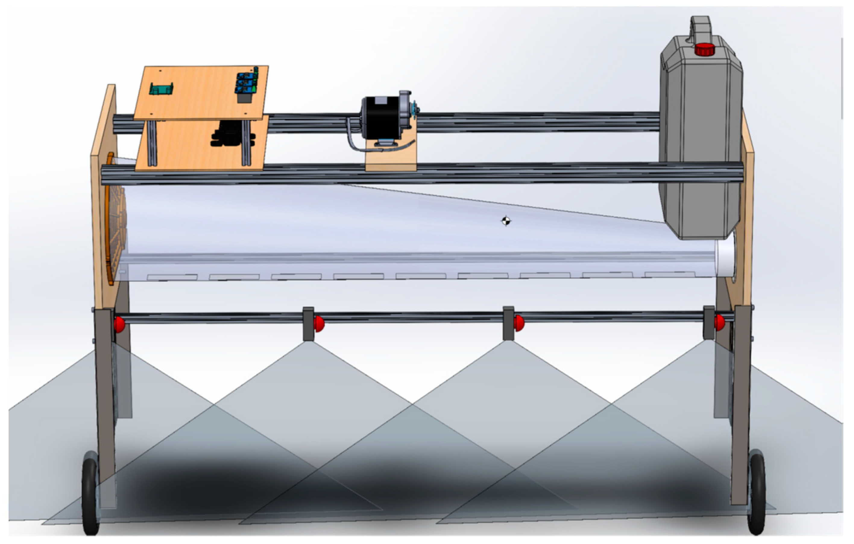
The main subsystems of the designed machine are: data gathering, spraying circuit, boom structure and actuation, rover structure and motion, and navigation computing/electronics. The aim of the data gathering subsystem is to acquire information regarding the plant and the treatment, carried out thanks to a 3D camera, a pressure sensor and a flow sensor. The 3D camera is by far the most important component, both in terms of information output and cost; its core function is to determine the type and growth stage of the plant, while allowing a visual odometer to measure the speed of the rover, a fundamental parameter for the treatment. The water pressure and flow sensors instead allow a closed-loop control of the droplet size and product amount. While in theory the pressure-flow curve of the nozzles is known, and therefore only one of these sensors would be needed, the presence of both allows to detect faults (clogged nozzles, disconnected pipes, air in the pump, etc.) and consequently stop the treatment, thus allowing the user to solve the problem immediately.

The spraying circuit is the subsystem with the more traditional architecture. The water line starts from the plastic tank and, through a high-pressure (up to 8 bar) variable speed membrane pump, delivers the water to the nozzles. To allow different spacing, two rows of nozzles were installed, driven by an electrovalve to allow using only one row, so resulting in a 50 cm distance between active nozzles, or both, reducing this distance to 25 cm. The 50 cm distance was considered because it is the standard generally adopted on sprayer booms, while the addition of the second row allows multiangle treatment and lower dispersion of the droplets when reducing the boom height from the ground. A low-pressure (0.2 bar) agitation pump recirculates the water in the tank, to avoid sedimentation when a powder-based of PPP is used. The air line is composed only of a variable speed fan and a flexible plastic air sleeve to direct the flow over the treatment area.

The boom structure is an aluminum body-on-frame. The selection of aluminum as the main material, despite the higher cost, is due to the necessity to keep this component as light as possible since the overhang outside the track and the height from the ground have to be adjustable. To change the height, within a range of 30 cm, a linear electric actuator was used, to cover the optimal settings for both the defined nozzle distances.

The rover structure is a mild steel body-on-frame, coated with high-temperature powder paint to increase durability. Due to the low working speed, no suspension system was implemented. The rear wheels have independent in-hub motors, while the front wheels are free-pivoting. This configuration allows controlling the motion without a steering system, by imposing the speed of the right and left wheel. The motors are driven from two independent power drives that implement a closed-loop speed control and are directly connected to the battery. The battery is a 48 V Li-ion pack with a waterproof casing. For a suitable safety of the operations, an emergency switch is put on the battery for the disconnection.

The navigation system is based on a differential real-time kinematic GPS. This system consists of three sensors and antennas, two on the rover and one in a fixed reference position on the ground. Thanks to the real-time kinematic algorithm the relative position of the antennas can be known with precision in the subcentimetric range. The two antennas on the rover allows to determine differentially its spatial orientation, with a typical uncertainty of 0.2°. The data coming from the GPS are fused with those obtained from the inertial measurement unit (IMU) and the 3D camera, to allow excellent accuracy and to stop safely the system in case of malfunctions. The data taken from all the navigation sensors, as well as the data gathering subsystem, are then collected and elaborated from the main computing unit, a Linux-based x86 Personal Computer (PC), to determine the movement and treatment actuator response. The PC is paired with a microcontroller and a power unit to electrically interface with the sensors and actuators. A separate power supply is used for the PC, while the microcontroller board is powered directly through the PC. To evaluate the potential of this solution, a prototype has been designed and built to run on-field tests to define the optimal way of spraying, given the characteristics of the plants.

2.2. Prototype

To verify the potential of the prototype, an advanced boom equipped with the camera was realized before the complete rover, to test the sprayer while varying all the considered parameters, and therefore to validate the reduction of the pesticide usage. In this paper, the detailed design of the advanced boom and the results of its validation are reported, before any industrialization step. Focusing on advanced boom validation instead of the full system, allowed to manage properly the basic functionalities. In particular, the prototype detailed in this paper includes:

• A simplified structure made with wooden panels, while the actuation of the boom was eliminated, and the “legs” of the prototype were used to manually change the height between tests.
• A small tank, of 20 L capacity, however sufficient for carrying out several test sets.
• No flow sensors: new nozzles are used, the nominal flow rate is therefore known and so no pressure sensor is needed to obtain all the flow parameters.
• No navigation hardware. The testing will be carried out in a straight line.
• Laptops instead of a dedicated embedded PC.
• A main power supply instead of a battery. Moreover, due to the reduced power, the main circuit voltage was reduced from 48 V to 12 V.
• A geared motor instead of the in-hub motors. The gear was used to drive a chain with one extremity fixed to the wall and so regulate the test bench speed.
• Two cheap pumps have been used instead of a professional model. The quality of the pump is not relevant to the test results since the flow conditions are directly imposed.

The CAD model (Figure 1) shows the design and the overall structure of the test bench manufactured for quantitative evaluation of the proposed solution.

2.3. Field Tests

The main goal was to test the prototype in different working conditions considering various operating parameters, to find the most suitable spraying setting in given crop conditions. Two test sessions were carried out, as the pesticides are distributed at different stages of the plants’ growth. The height and the width of the salad leaves were taken into account as representative of the crop. In detail, the parameters investigated were:

• the nozzles’ typology: the nozzle type affects the drops’ dimension;
• nozzle distance: the distance affects the area covered by the drops, and in particular the spraying overlap between the adjacent nozzles, in order to obtain the maximum distribution uniformity;
• nozzle height: the height of the nozzles from the top of the crop affects the size of the drop-covered area;
• rover speed: the speed affects the amount of mixture distributed on a given surface;
• pressure: the variation of the spraying pressure changes the drop size, affecting the coverage of the crop, but also the possible drift of the mixture.

A total of 37 tests were carried out, arranging different combinations of the shown features. To check the amount and evaluate the spraying features, 75 water-sensitive papers were used for each test; the sensitive papers were placed in the crop in predefined ways, and after each run collected and analyzed. A depth camera was used to record each test and an image processing algorithm has been implemented to identify the plants and measure height and covered area.

For the tests, radicchio (Cichorium intybus L.) was selected as the main crop, being representative of most used salads in the ready-to-eat salad sector.

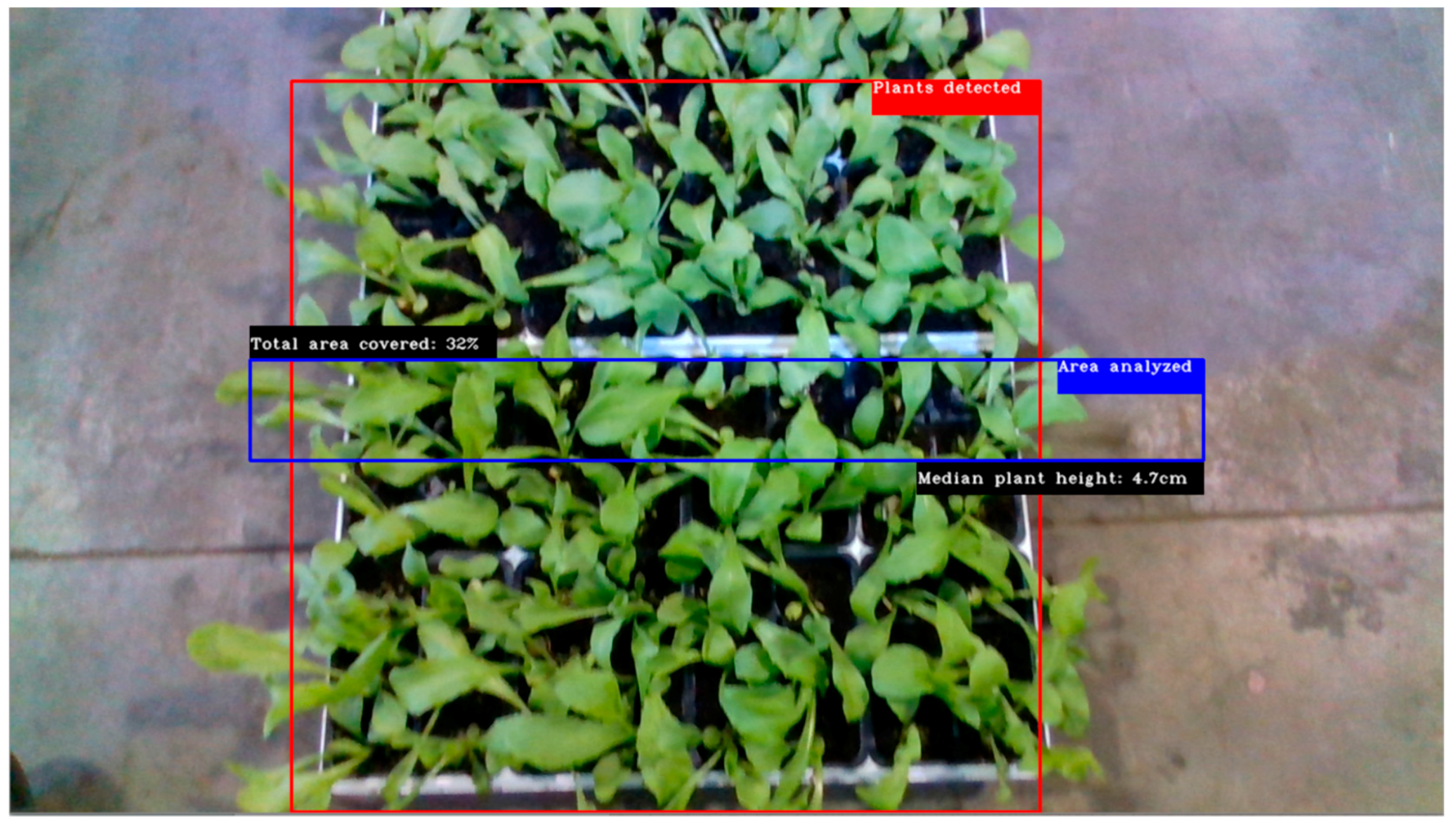
2.3.1. Real-Time Measurement of the Plants’ Features

The camera used for the tests is the Intel RealSense™ Depth Camera D435i [12]. Apart the relatively low cost (about 200 $), this model allows at the same time to measure distances and to collect images; moreover, this specific model is equipped with an integrated IMU sensor. The algorithm for image processing has been implemented in C++ via the RealSense library [13], as it contains all the functions needed to use the camera.

The algorithm structure for image processing implements a classical pipeline. At first, some filters [14] are defined and applied to the data acquired by the camera, to reduce the noise and improve image quality, as follows:

• decimation filter: the resolution of the depth scene is reduced to reduce the necessary computation power;
• spatial filter: an edge-preserving filter with a performance that can be used in real-time;
• temporal filter: a filter that uses the information of the previous frames to adjust the current frame. This is a useful function, above all in static conditions.

After data acquisition and filtering, color detection and segmentation algorithms were used to find the plants. The OpenCV library [15] has been used to implement a simple algorithm [16] assuming, in a greenhouse scenario, the most common salad color is in the range of green, while the terrain is typically earth brown. Based on this simple assumption, it was necessary to find the right range of greens to detect the plants; although a possible solution could have been to work in the red, green, and blue (RGB) domain [17], since the frames were already in this format, the color values of this domain are extremely sensitive to light intensity, and therefore the best option was to convert each frame into the hue saturation value (HSV) domain [18]. Once the RGB frame is converted into HSV, a binary mask is computed to find where a specified color is.

As the tests were not conducted in a greenhouse, the assumption on the contrast between the salads’ and the terrain’s colors was not valid, and we had to tune the range also considering the background of the images, containing grey (the floor color). Due to some reflection, this grey area in the HSV analysis presented some “yellow” components, very close to the “green” part of the HSV spectrum; the choice of a proper threshold turned in to exclude some parts of the salads not to detect erroneously the ground. For real applications in greenhouse this should not happen, because of the clearer distinction between the color of the terrain and the salads.

Knowing where the plants are, it is possible to extract useful information like the height of the plants, from the depth component of the camera, and the percentage of the covered area. To work in real-time, some additional information on the plants is needed; indeed, to reduce the computational power of the algorithm and increase the throughput, the analysis is performed on a smaller area of the frame chosen in the middle of the frame, with a height which is one eighth of the total height of the image and a width that is two-thirds of the frame width. In Figure 2, the red rectangle identifies the plants detected, while the blue one indicates the area analyzed. Assuming the plants we want to analyze are in the middle of the frame, the algorithm measures the distance of the floor/terrain using a strip to the left and a strip to the right of the area under analysis. In doing this, all the “green” pixels are discarded, while the other measures are stored in a vector. The same process is done also for the plants: the algorithm considers all the pixels that are in the intersection of the area under analysis (the blue rectangle) and where the plants are identified; if the pixel is green, the distance is stored in another vector.

Having two vectors, respectively, for the distance measurements of the floor and the distance measurements of the plants, we compute the floor and plant distances using the median of the available samples as the mean would have been too sensible to the presence of several outliers. In a greenhouse scenario, the availability of these two values is sufficient to compute the median height of the plants in the area taken into account for the analysis. During the laboratory tests, the plants were placed in some trays, thus, the algorithm measures the height of the plants as:

median_plant_height = median_floor_distance − median_plants_distance − trays_height
(trays_height = 0.06 m).

The vision algorithm measures also the percentage of the analyzed area covered by the plants counting the number of green pixels recognized as plants and computes the ratio between this number and the total number of pixels inside the area. This last method uses 2D information, thus it does not extract volumetric characteristics of the plants.

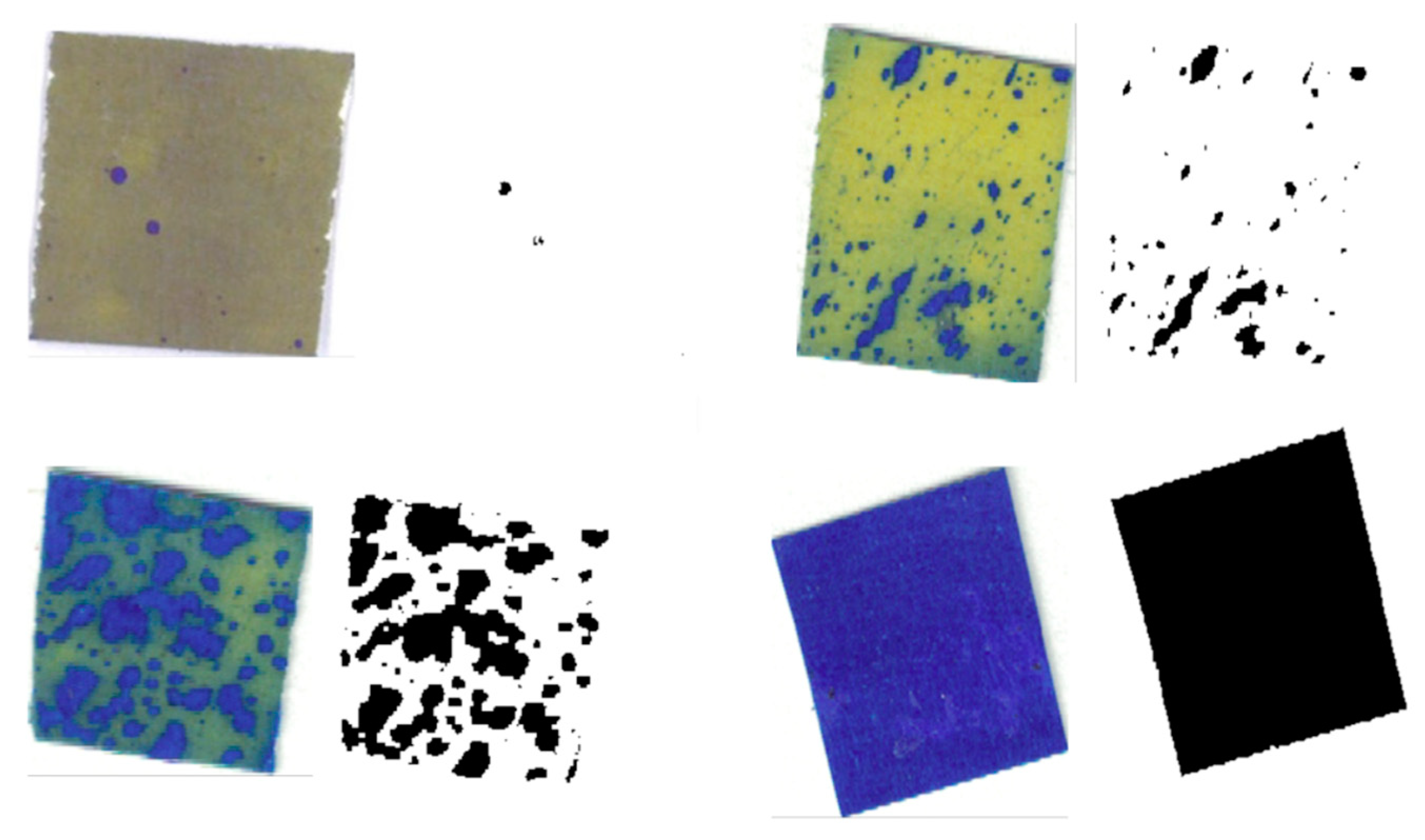
2.3.2. Evaluation of the Spraying Quality and the Amount of Spray Liquid (Water) Used

Seventy-five square-shaped water-sensitive papers of about 1 cm² area were placed on the upper surface of leaves (25 samples), on the lower surface (25 samples), and on the ground (25 samples). Salads were planted in eight bedding plant trays, each containing 6 × 8 smaller trays, each of them containing a plant. The dry water-sensitive papers were gently stuck to the plant leaf using a natural glue, and these remained there after the end of the treatment (i.e., the passage of rover with spraying water on the eight trays), including the time needed for the plants and papers to become dry again.

To perform a more systematic analysis and obtain quantitative results, the samples were classified and then attached to a blank A4 paper for image processing. A dedicated algorithm was used to extract every single water-sensitive paper and to perform the color analysis.

Dry water-sensitive papers are typically yellow, but when completely wet become blue. The parts of papers not well sprayed become light blue. The image processing algorithm is able to detect pixels with sufficient color saturation, meaning that they are close to the blue threshold value, defined from the sample of scanned papers. Since the samples were not perfectly squared and their area was not exactly 1 cm², and during gluing them on white A4 paper they could not be perfectly aligned, the image to be processed also needed detection of all other nonwhite colors (Figure 3). This way, a few parameters were introduced, defined for every single extracted water-sensitive sample:

• $N_{total}$ is the number of nonwhite pixels, i.e., the number of pixels in a 2D image representing the water-sensitive paper.
• $N_{blue}$ is the number of blue pixels, i.e., those pixels in the 2D image of the water-sensitive paper that represent parts of the paper covered by water.
• $x_{c,total}$ is the x coordinate of the geometric center of all nonwhite pixels in the 2D image.
• $y_{c,total}$ is the y coordinate of the geometric center of all nonwhite pixels in the 2D image.
• $x_{c,blue}$ is the x coordinate of the geometric center of all blue pixels in the 2D image.
• $y_{c,blue}$ is the y coordinate of the geometric center of all blue pixels in the 2D image.
• $c=\frac{N_{blue}}{N_{total}}$ is the coverage, can be expressed in percentage as $\frac{N_{blue}}{N_{total}}\times 100\%$ indicates what percentage of the area of the water-sensitive paper is covered by water or, in more practical terms, sprayed well.
• d = $\sqrt{{\left(X_{c,blue}-X_{c,total}\right)}^2+{\left(Y_{c,blue}-Y_{c,total}\right)}^2}$ is the distance (offset) between the two geometric centers defined above; the lower the value, the more centered spraying is performed.

The final output of the water-sensitive papers analysis algorithm is a report containing the following parameters for each test and each region (specific position—upper leaf, lower leaf, ground):

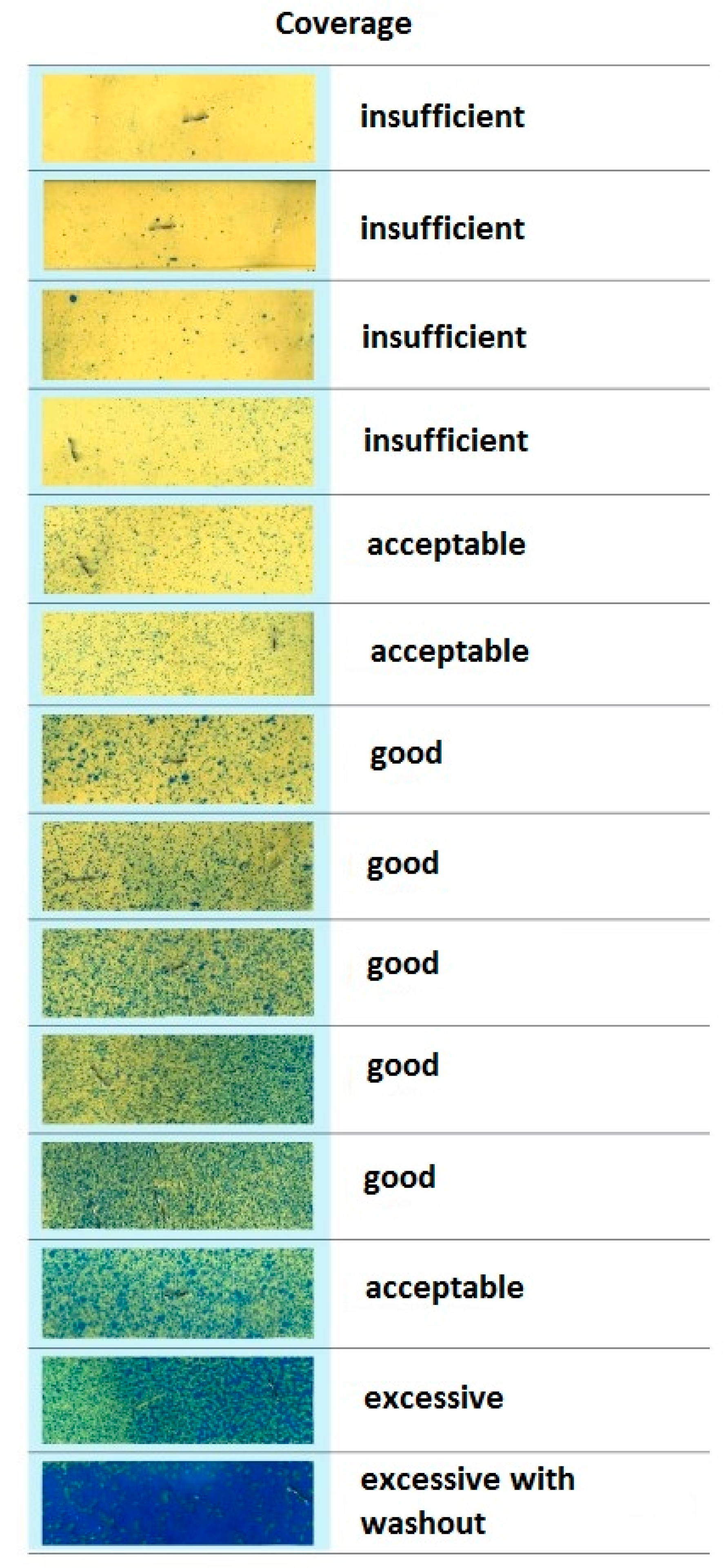
• $N_{insufficient}$ is the number of insufficiently sprayed samples, i.e., those papers for which the coverage $c$ is below the adopted threshold $t=7\%$. The threshold value was adopted experimentally, after running the program for different values and comparing with the exemplary papers from reference [19].
• $N_{sufficient}$ is the number of all other samples from the same test and region; in total $N=N_{sufficient}+N_{insufficient}\le 25$ is the number of papers in a single test, from a single specific region.
• $\overline{c}$ is the average coverage for the single test, defined as $\overline{c}=\frac{\stackrel{N}{\underset{i=1}{\sum c_i}}}{N}$, $c_i$ is the coverage of every single water-sensitive paper belonging to this test and region.
• ${\sigma }_c=\sqrt{\frac{{\sum }_{i=1}^N {\left(c_i-\overline{c}\right)}^2}{N}}$ is the standard deviation of coverage for the given test and region.
• $\overline{d}$ is the average distance (offset) for the single test, defined as: $\overline{d}=\frac{\stackrel{N}{\underset{i=1}{\sum d_i}}}{N}$, where $d_i$ is the offset for every single water-sensitive sample belonging to the considered test and region.
• ${\sigma }_d=\sqrt{\frac{{\sum }_{i=1}^N {\left(d_i-\overline{d}\right)}^2}{N}}$ is the standard deviation of distance (offset) for the given test and region.

Another important aspect of the analysis is the amount of mixture (water) distributed. It can be estimated, knowing the flow rate of each nozzle, the speed at which the rover moves and, to refer to the area covered, the distance between the nozzles. Such quantity, called “coverage”, is defined as

$$C=\left(\raisebox{1ex}{$l$}\!\left/ \!\raisebox{-1ex}{$ha$}\right.\right)=\frac{Q}{v\Delta s}\times {10}^4$$

(1)

where:

• $Q \left(\raisebox{1ex}{$l$}\!\left/ \!\raisebox{-1ex}{$s$}\right.\right)$ is the nozzle flow rate
• $v\left(\raisebox{1ex}{$m$}\!\left/ \!\raisebox{-1ex}{$s$}\right.\right)$ is the travelling speed of the rover
• $\Delta s\left(m\right)$ is the distance between the nozzles.

To calculate the flow rate, the following equation is adopted:

$$Q=const.\times \sqrt{\Delta p},$$

(2)

where:

• $\Delta p$ is the differential pressure between the pressure of fluid inside the nozzle and ambient pressure; this differential pressure is directly obtained from the sensor.

Using table data for the flow at $\Delta p=300 kPa$, it is possible to express:

$$Q\left(\Delta p\right)=Q\left(300 kPa\right)\times \sqrt{\frac{\Delta p}{300 kPa}}.$$

(3)

For choosing the optimal set of spraying parameters, both the following conditions should be met:

• Average coverage $\overline{c} (\%)$ should be acceptable (not too low, and with no or very few insufficient papers, Figure 4).
• Coverage in liters per hectare $C \left(\raisebox{1ex}{$L$}\!\left/ \!\raisebox{-1ex}{$ha$}\right.\right)$ should be as low as possible.

It is intuitively clear that these parameters are, roughly speaking, inversely correlated.

3. Results and Discussion

The results of all the 37 tests are shown in

Table A1. Results of all the tests.

Test	${\mathit{N}}_{\mathit{s}\mathit{u}\mathit{f}}$	${\mathit{N}}_{\mathit{i}\mathit{n}\mathit{s}\mathit{u}\mathit{f}}$	$\overline{\mathit{c}} (\mathbf{\%})$	${\mathit{\sigma }}_{\mathit{c}} (\mathbf{\%})$	$\overline{\mathit{d}}$	${\mathit{\sigma }}_{\mathit{d}}$	$\mathit{C} \left(\mathit{l}/\mathit{h}\mathit{a}\right)$
1-upper	25	0	94.2	3.2	1.89	1.58	952.0
1-lower	8	12	31	19.9	22.62	24.80	952.0
1-ground	24	0	96.8	1.1	0.65	0.88	952.0
2-upper	25	0	85.8	12.0	4.67	4.15	426.0
2-lower	24	1	78.5	18.3	6.68	6.20	426.0
2-ground	24	0	96.6	1.5	0.86	1.49	426.0
3-upper	25	0	77.5	18.8	9.11	6.96	662.4
3-lower	11	13	36.3	21.0	43.09	21.63	662.4
3-ground	25	0	95.5	2.7	1.34	1.87	662.4
4-upper	23	2	38.9	17.8	12.78	9.03	435.0
4-lower	8	15	18.7	10.0	22.44	10.65	435.0
4-ground	25	0	96.7	0.8	0.66	0.47	435.0
5-upper	22	1	45.9	16.6	7.82	5.40	466.2
5-lower	8	15	35.4	23.3	13.72	9.02	466.2
5-ground	25	0	96.6	1.0	0.68	0.65	466.2
6-upper	25	0	78.6	14.3	4.54	3.27	447.9
6-lower	5	19	20.6	9.8	11.62	9.08	447.9
6-ground	25	0	96.6	1.4	0.87	0.99	447.9
7-upper	22	1	45.9	16.5	8.02	5.49	584.0
7-lower	8	15	35.2	23.3	13.79	9.24	584.0
7-ground	25	0	96.6	1.0	0.68	0.65	584.0
8-upper	25	0	78.8	19.5	6.32	6.35	622.5
8-lower	19	4	62.0	26.5	14.45	11.69	622.5
8-ground	25	0	96.7	1.5	0.67	0.69	622.5
9-upper	25	0	85.8	12.0	4.67	4.15	426.0
9-lower	24	1	78.5	18.3	6.68	6.20	426.0
9-ground	24	0	96.6	1.5	0.86	1.49	426.0
10-upper	25	0	75.9	28.3	5.46	6.21	492.2
10-lower	18	5	55.0	27.1	13.86	11.85	492.2
10-ground	24	0	96.9	1.0	0.47	0.47	492.2
11-upper	22	3	62.0	17.8	9.97	6.44	306.8
11-lower	7	18	17.5	14.6	31.15	25.59	306.8
11-ground	24	0	97.3	0.6	0.37	0.24	306.8
12-upper	24	1	73.1	30.4	8.73	11.65	440.0
12-lower	7	18	53.8	25.8	15.37	11.27	440.0
12-ground	21	0	97.1	0.6	0.48	0.33	440.0
13-upper	24	0	84.0	22.7	6.15	11.55	438.0
13-lower	21	3	81.6	15.0	6.25	5.04	438.0
13-ground	23	0	95.4	4.7	1.73	4.23	438.0
14-upper	23	0	95.2	4.4	1.39	1.82	469.6
14-lower	21	1	84.1	15.7	6.73	10.54	469.6
14-ground	21	0	97.0	0.5	0.42	0.27	469.6
15-upper	21	1	57.8	30.8	13.39	13.67	438.0
15-lower	18	5	75.4	24.6	8.47	12.24	438.0
15-ground	25	0	91.6	16.8	4.17	14.36	438.0
16-upper	14	10	34.9	18.5	14.71	10.79	354.8
16-lower	7	12	21.6	12.2	29.80	17.04	354.8
16-ground	24	0	94.1	1.8	2.01	1.26	354.8
17-upper	24	0	75.0	27.6	9.50	13.41	441.8
17-lower	22	1	81.5	26.4	7.00	14.33	441.8
17-ground	25	0	95.1	0.8	1.14	0.62	441.8
18-upper	20	4	49.2	25.0	13.64	10.01	404.7
18-lower	15	5	36.7	23.1	24.63	18.50	404.7
18-ground	25	0	94.9	1.1	1.34	1.04	404.7
19-upper	18	6	49.9	31.7	13.50	13.98	432.5
19-lower	15	5	34.9	28.2	19.18	16.62	432.5
19-ground	25	0	94.2	1.9	1.70	1.53	432.5
20-upper	16	8	47.8	34.2	7.68	5.25	358.8
20-lower	10	15	28.5	26.8	24.38	17.02	358.8
20-ground	24	0	94.1	2.2	2.02	1.56	358.8
21-upper	24	0	67.1	28.3	11.41	9.55	435.3
21-lower	21	4	68.1	29.5	13.31	14.26	435.3
21-ground	24	0	94.1	2.9	1.94	2.32	435.3
22-upper	16	4	54.9	32.0	15.36	16.23	422.4
22-lower	20	3	56.8	33.2	13.84	14.64	422.4
22-ground	25	0	92.6	2.8	2.22	1.49	422.4
23-upper	23	0	94.0	4.3	2.03	2.37	379.8
23-lower	23	0	94.4	4.8	3.16	3.37	379.8
23-ground	25	0	93.1	4.6	3.68	3.77	379.8
24-upper	25	0	95.7	2.2	1.47	1.70	456.7
24-lower	21	0	95.8	2.8	1.52	1.59	456.7
24-ground	24	0	96.4	1.0	1.35	0.89	456.7
25-upper	23	0	93.3	13.6	2.06	4.21	347.1
25-lower	23	0	92.0	15.2	2.92	4.72	347.1
25-ground	23	0	96.0	1.4	1.65	1.13	347.1
26-upper	16	9	38.9	28.8	22.23	18.47	247.9
26-lower	19	5	42.2	30.3	21.65	13.09	247.9
26-ground	22	0	94.3	4.9	2.24	3.50	247.9
27-upper	22	2	62.4	32.7	16.94	17.40	265.5
27-lower	22	2	77.8	29.1	8.90	14.47	265.5
27-ground	20	0	94.7	4.4	2.61	3.22	265.5
28-upper	23	2	72.1	30.4	9.67	14.47	380.5
28-lower	17	5	53.8	34.8	20.35	21.11	380.5
28-ground	20	0	96.6	0.5	0.80	0.38	380.5
29-upper	16	6	72.5	20.8	13.23	12.99	344.2
29-lower	22	2	82.0	23.4	8.69	14.13	344.2
29-ground	25	0	96.6	0.8	0.94	0.53	344.2
30-upper	25	0	83.3	22.0	5.44	8.62	957.6
30-lower	21	2	86.2	20.5	4.68	7.34	957.6
30-ground	25	0	96.9	0.7	0.55	0.33	957.6
31-upper	19	4	70.2	21.8	7.83	6.74	650.4
31-lower	15	9	46.0	28.4	19.45	17.35	650.4
31-ground	24	0	94.7	7.2	1.60	3.08	650.4
32-upper	22	3	79.6	26.6	8.01	13.98	697.3
32-lower	16	9	71.8	32.2	14.23	22.95	697.3
32-ground	22	0	94.2	5.3	1.22	0.78	697.3
33-upper	22	3	53.8	25.1	9.52	10.19	440.5
33-lower	14	10	42.4	29.5	10.24	9.05	440.5
33-ground	22	0	96.1	1.5	0.87	1.07	440.5
34-upper	22	1	76.7	28.7	5.78	6.94	284.3
34-lower	21	2	79.7	26.9	7.37	12.09	284.3
34-ground	24	0	96.7	0.6	0.68	0.27	284.3
35-upper	22	2	60.8	34.5	8.82	11.26	372.8
35-lower	14	11	48.2	30.9	23.40	16.06	372.8
35-ground	24	0	97.0	0.4	0.60	0.26	372.8
36-upper	21	3	54.4	28.3	9.08	13.00	192.0
36-lower	12	8	51.7	37.7	18.05	23.76	192.0
36-ground	24	0	95.6	4.8	1.48	3.86	192.0
37-upper	18	6	60.8	24.2	13.68	13.62	330.9
37-lower	13	10	61.3	30.7	12.27	12.38	330.9
37-ground	21	0	96.1	1.0	1.00	0.55	330.9

and

Table A2. Selected parameters of all 37 tests.

Test Number	1	2	3	4	5	6	7	8
Height (cm)	65	65	65	65	65	53	53	53
Nozzle distance (cm)	50	50	50	50	50	40	40	40
Number of nozzles	2	2	2	2	2	3	3	3
Nozzle type (l/min) at 300 kPa	2.4	1.6	1.6	1	0.8	0.8	0.8	0.8
Nozzle inclination (°)	2	2	−22	−22	−22	−22	−22	−22
Air inclination (°)	0	0	0	0	0	0	0	0
Speed (km/h)	2.45	2.45	2.50	2.51	2.35	2.45	2.45	2.00
Pressure (kPa)	197.5	216.7	223.2	248.7	390.0	251.8	428.1	322.9
Flow (l/min)	1.95	1.36	1.38	0.91	0.91	0.73	0.96	0.83
Average plant height (cm)	7	7	7	7	7	7	7	7
PWM1motor (%)	100	100	100	100	100	100	100	80
PWM1pump (%)	77	60	60	45	52	52	77	62
Test Number	9	10	11	12	13	14	15	16
Height (cm)	53	53	53	27	27	27	27	37
Nozzle distance (cm)	40	50	50	50	25	25	25	25
Number of nozzles	3	3	2	2	3	3	3	3
Nozzle type (l/min) at 300 kPa	0.8	0.8	0.8	0.8	0.8	0.8	0.8	0.8
Nozzle inclination (°)	0	0	0	0	20	−20	−20	−20
Air inclination (°)	30	30	30	30	30	30	30	30
Speed (km/h)	2.25	2.25	3.60	4.15	4.15	3.86	3.91	3.86
Pressure (kPa)	191.4	399.3	397.0	271.8	269.4	267.0	239.0	152.4
Flow (l/min)	0.64	0.92	0.92	0.76	0.76	0.75	0.71	0.57
Average plant height (cm)	7	7	7	7	7	7	14	14
PWM1motor (%)	100	100	73	100	100	100	100	100
PWM1pump (%)	77	84	84	55	55	55	55	55
Test Number	17	18	19	20	21	22	23	24
Height (cm)	37	37	37	49	49	49	49	49
Nozzle distance (cm)	25	25	25	50	40	50	50	50
Number of nozzles	3	3	3	2	3	2	2	2
Nozzle type (l/min) at 300 kPa	0.8	0.8	0.8	0.8	0.8	1.0	1.2	0.8
Nozzle inclination (°)	0	45, −45	45, −45	−20	−20	−20	−20	0
Air inclination (°)	30	30	30	0	0	0	0	24
Speed (km/h)	4.32	3.86	3.62	2.51	2.51	2.70	3.97	3.12
Pressure (kPa)	296.4	198.3	199.9	264.3	249.0	271.0	329.0	661.4
Flow (l/min)	0.80	0.65	0.65	0.75	0.73	0.95	1.26	1.19
Average plant height (cm)	14	14	14	14	14	14	14	14
PWM1motor (%)	100	100	100	68	68	68	100	80
PWM1pump (%)	60	45	45	39	52	47	60	84
Test Number	25	26	27	28	29	30	31	32
Height (cm)	49	49	49	49	65	65	65	65
Nozzle distance (cm)	50	50	50	25	50	50	50	50
Number of nozzles	2	2	2	3	2	2	2	2
Nozzle type (l/min) at 300 kPa	0.8	0.6	0.6	0.6	0.6	2.4	1.6	1.6
Nozzle inclination (°)	0	0	0	45, −45	20	0	0	−20
Air inclination (°)	30	30	30	30	30	0	0	0
Speed (km/h)	3.18	3.38	3.48	4.15	3.00	2.57	2.45	2.35
Pressure (kPa)	395.6	405.0	495.0	361.5	617.1	219.3	207.4	218.1
Flow (l/min)	0.92	0.70	0.77	0.66	0.86	2.05	1.33	1.36
Average plant height (cm)	14	14	14	14	14	14	14	14
PWM1motor (%)	80	90	80	100	100	62	62	62
PWM1pump (%)	52	45	52	56	65	75	56	58
Test Number	33		34	35		36	37
Height (cm)	65		65	49		49	49
Nozzle distance (cm)	50		50	50		50	50
Number of nozzles	2		2	2		2	2
Nozzle type (l/min) at 300 kPa	0.8		1.0	1.2		0.6	0.8
Nozzle inclination (°)	−20		−20	−20		−20	0
Air inclination (°)	0		0	0		30	30
Speed (km/h)	2.45		4.00	4.06		3.72	3.29
Pressure (mbar)	380.6		269.4	331.4		2959	3865
Flow (l/min)	0.90		0.95	1.26		0.60	0.91
Average plant height (cm)	14		14	14		14	14
PWM1motor (%)	62		100	100		100	80
PWM1pump (%)	51		46	60		36	52

¹ pulse width modulation.

(Appendix A) and analyzed according to the different parameters defined in the previous section: $N_{sufficient}$, $N_{insufficient}$, $\overline{c},$ ${\sigma }_c$, $\overline{d}, {\sigma }_d$, $C.$ Columns are defined by these parameters, and for each test three rows were reserved for upper leaves, lower leaves, and ground.

Results for the water-sensitive samples collected from the ground showed that the spraying was carried out in all conditions at an almost complete coverage, thus suggesting not to focus on this information. This was expected, so the third (’ground’) row of each test put in the table is not significant.

After applying the criterion for the number of “insufficient papers”, only 10 tests remained for further consideration, which accounts for roughly 250 samples. The mixture (water) amount ranged from the very promising value of 265.5 L/ha to standard treatment of 957.6 L/ha (i.e., very close to the theoretical 1000 L/ha). Considering this work aimed to show the possibility to reduce significantly the pesticide distribution while maintaining good or even improving spraying results, it has been decided to go deep only in those tests involved in a distribution of less than 500 L/ha. The relevant results are shown in

Table 1. The selected results from the first (nos. 9, 13, 14) and the second test session (nos. 17, 21, 24, 27, 34).

Test	${\mathit{N}}_{\mathit{s}\mathit{u}\mathit{f}}$	${\mathit{N}}_{\mathit{i}\mathit{n}\mathit{s}\mathit{u}\mathit{f}}$	$\overline{\mathit{c}} (\mathbf{\%})$	${\mathit{\sigma }}_{\mathit{c}} (\mathbf{\%})$	$\overline{\mathit{d}}$	${\mathit{\sigma }}_{\mathit{d}}$	$\mathit{C} \left(\mathit{l}/\mathit{h}\mathit{a}\right)$
9-upper	25	0	85.8	12.0	4.67	4.15	426.0
9-lower	24	1	78.5	18.3	6.68	6.20	426.0
9-ground	24	0	96.6	1.5	0.86	1.49	426.0
13-upper	24	0	84.0	22.7	6.15	11.55	438.0
13-lower	21	3	81.6	15.0	6.25	5.04	438.0
13-ground	23	0	95.4	4.7	1.73	4.23	438.0
14-upper	23	0	95.2	4.4	1.39	1.82	469.6
14-lower	21	1	84.1	15.7	6.73	10.54	469.6
14-ground	21	0	97.0	0.5	0.42	0.27	469.6
17-upper	24	0	75.0	27.6	9.50	13.41	441.8
17-lower	22	1	81.5	26.4	7.00	14.33	441.8
17-ground	25	0	95.1	0.8	1.14	0.62	441.8
21-upper	24	0	67.1	28.3	11.41	9.55	435.3
21-lower	21	4	68.1	29.5	13.31	14.26	435.3
21-ground	24	0	94.1	2.9	1.94	2.32	435.3
24-upper	25	0	95.7	2.2	1.47	1.70	456.7
24-lower	21	0	95.8	2.8	1.52	1.59	456.7
24-ground	24	0	96.4	1.0	1.35	0.89	456.7
27-upper	22	2	62.4	32.7	16.94	17.40	265.5
27-lower	22	2	77.8	29.1	8.90	14.47	265.5
27-ground	20	0	94.7	4.4	2.61	3.22	265.5
34-upper	22	1	76.7	28.7	5.78	6.94	284.3
34-lower	21	2	79.7	26.9	7.37	12.09	284.3
34-ground	24	0	96.7	0.6	0.68	0.27	284.3

; to offer full insights, in

Table 2. Parameters from the tests 9, 13, 14, 17, 21, 24, 27 and 34.

Test Number	9	13	14	17	21	24	27	34
Height (cm)	53	27	27	37	49	49	49	65
Nozzle distance (cm)	40	25	25	25	40	50	50	50
Number of nozzles	3	3	3	3	3	2	2	2
Nozzle type (l/min) at 300 kPa	0.8	0.8	0.8	0.8	0.8	0.8	0.6	1
Nozzle inclination (°)	0	20	−20	0	−20	0	0	−20
Air inclination (°)	30	30	30	30	0	30	30	0
Speed (km/h)	2.25	4.15	3.86	4.32	2.51	3.12	3.48	4.00
Pressure (mbar)	1914	2694	2670	2964	2490	6614	4950	2694
Flow (l/min)	0.64	0.76	0.75	0.80	0.73	1.19	0.77	0.95
Average plant height (cm)	7	7	7	14	14	14	14	14
PWM1motor (%)	100	100	100	100	68	80	80	100
PWM1pump (%)	77	55	55	60	52	84	52	46

¹ pulse width modulation.

all the parameters affecting the results are shown.

In Table 1, some runs show a slightly higher standard deviation ${\sigma }_c$. Although they have very good coverages $\overline{c}$, these values may suggest that by repeating the tests with the same parameters different results (possibly worse) could be obtained. To select the optimal parameters, we could have used the simple index of performance defined as $\eta =\raisebox{1ex}{$c$}\!\left/ \!\raisebox{-1ex}{$C$}\right.$ could have been used. Although this makes sense as it represents the percentage coverage $c (\%)$ reached with a certain amount in L/ha, it is necessary to consider that the variance plays an important role. For this reason, we excluded to the time being very promising results (i.e., less than 300 L/ha) as they need further investigation.

Staying on the safe side, we can reliably state that with 420–470 L/ha it was possible to obtain excellent coverage of upper and lower leaves in both test sessions (for example, tests nos. 9 and 14 from the first session, with an average plant height of 7 cm and test no. 24 from the second session, with an average plant height of 14 cm).

Considering a theoretical mixture amount of 1000 L/ha, these numbers show that it is possible to optimize spraying parameters with a reduction of more than 50%. Going down to less than 470 L/ha, coverage results are however excellent, and still remain promising opportunities to reduce the usage below 300 L/ha, starting from the parameters of tests nos. 27 and 34 (Table 2).

4. Conclusions

Given that the commonly distributed mixture (amount of spray liquid for pesticide treatments) for the cultivation of ready-to-eat salads is 1000 L/ha, the tests carried out produced extremely promising results. Through the optimization of setting parameters, in the first life stage of the plant it is possible to decrease that amount up to 426 L/ha, maintaining an excellent coverage of the vegetation, with a very low wasting of PPPs to the ground. In a further stage of the plants growth, the optimal amount turned out to be 460 L/ha, still more than half of the standard.

The solution described will result in many benefits, ranging from environmental to economic sustainability. First, the overall treatment requires 55% less pesticide product and, consequently, chemicals will not be wasted anymore, avoiding soil and groundwater pollution. Furthermore, the usage of an electric rover replacing the diesel tractor will decrease the pollutant gas emission, also avoiding fossil fuel consumption and reducing CO₂ emissions.

Future studies should strive to explore additional improvements in pesticide usage with other parameters settings as, from the tests, very promising results have been obtained also below the proposed setting reaching 265.5 L/ha use.

References

1. How to Feed the World 2050, High-Level Expert Forum FAO. Available online: http://www.fao.org/fileadmin/templates/wsfs/docs/Issues_papers/HLEF2050_Global_Agriculture.pdf (accessed on 11 December 2020).
2. The International Code of Conduct on Pesticides Management, FAO and WHO. Available online: http://www.fao.org/3/a-i3604e.pdf (accessed on 11 December 2020).
3. Pesticides, European Commission. Available online: https://ec.europa.eu/food/plant/pesticides_en (accessed on 14 December 2020).
4. Statistics on Pesticides Use in Agriculture, 1990–2018, FAO Environmental Statistics. Available online: http://www.fao.org/economic/ess/environment/data/pesticides-use/en/ (accessed on 12 December 2020).
5. Directive 2009/128/EC of the European Parliament and the Council of 21 October 2009. Available online: https://eur-lex.europa.eu/legal-content/EN/TXT/HTML/?uri=CELEX:02009L0128-20091125&from=EN (accessed on 14 December 2020).
6. Pesticides Use, FAOSTAT. Available online: http://www.fao.org/faostat/en/#home (accessed on 12 December 2020).
7. Agri-Environmental Indicator—Consumption of Pesticides, Eurostat. Available online: https://ec.europa.eu/eurostat/statistics-explained/index.php?title=Agri-environmental_indicator_-_consumption_of_pesticides#Data_sources (accessed on 12 December 2020).
8. Distribuzione per uso Agricolo dei Prodotti Fitosanitari (Erbicidi, Fungicidi, Insetticidi, Acaricidi e Vari), ISTAT. Available online: https://annuario.isprambiente.it/ada/downreport/html/6940 (accessed on 13 December 2020).
9. Italian Agriculture in Figures 2017, CREA. Available online: https://www.crea.gov.it/documents/68457/0/Itaconta+2017_+ING_DEF_WEB2.pdf/1218e51d-0bf5-03d0-3089-0a56af2e26d5?t=1559117850834 (accessed on 14 December 2020).
10. Gullino, M.L.; Gilardi, G.; Garibaldi, A. Ready-to-eat salad crops: A plant pathogen’s heaven. Plant Dis. 2019, 103, 2153–2170. [Google Scholar] [CrossRef] [PubMed] [Green Version]
11. Casati, D.; Baldi, L. L’importanza economica del comparto della IV gamma. In Le Malattie degli Ortaggi di IV Gamma; Sanninoand, L., Espinosa, B., Eds.; Inteli Press: Battipaglia, Italy, 2016; pp. 19–30. [Google Scholar]
12. Intel RealSense Depth Camera d435i. Available online: https://www.intelrealsense.com/depth-camera-d435i/ (accessed on 16 September 2020).
13. Intel RealSense SDK 2.0 Library. Available online: https://github.com/IntelRealSense/librealsense (accessed on 16 September 2020).
14. Intel RealSense SDK 2.0 Library: Post-Processing Filters. Available online: https://github.com/IntelRealSense/librealsense/blob/master/doc/post-processing-filters.md (accessed on 16 September 2020).
15. Open-Source Computer Vision Library. Available online: https://github.com/opencv/opencv (accessed on 21 September 2020).
16. OpenCV: Color Detection and Segmentation Example. Available online: https://www.learnopencv.com/invisibility-cloak-using-colordetection-and-segmentation-with-opencv/ (accessed on 17 September 2020).
17. RGB Color Model. Available online: https://en.wikipedia.org/wiki/RGB_color_model (accessed on 17 September 2020).
18. HSV Color Model. Available online: https://en.wikipedia.org/wiki/HSL_and_HSV (accessed on 21 September 2020).
19. Quaderno: Agricoltura Responsabile. Syngenta. 2014. Available online: https://www.syngenta.it/file/5031/download?token=NyHxitSm (accessed on 25 August 2020).
Figure 1. CAD model of the prototype.
Applsci 11 01992 g001
Figure 2. Image processing algorithm output.
Applsci 11 01992 g002
Figure 3. Some examples of single water-sensitive papers extracted by extraction algorithm (on the left in each pair) and black and white images obtained after transforming all ‘blue pixels’ to ‘black’ (on the right in each pair).
Applsci 11 01992 g003
Figure 4. Degree of coverage of water sensitive papers [19].
Applsci 11 01992 g004