Steady State Response of Linear Time Invariant Systems Modeledby Multibond Graphs

Abstract

The direct determination of the steady state response for linear time invariant (LTI) systems modeled by multibond graphs is presented. Firstly, a multiport junction structure of a multibond graph in an integral causality assignment (MBGI) to get the state space of the system is introduced. By assigning a derivative causality to the multiport storage elements, the multibond graph in a derivative causality (MBGD) is proposed. Based on this MBGD, a theorem to obtain the steady state response is presented. Two case studies to get the steady state of the state variables are applied. Both cases are modeled by multibond graphs, and the symbolic determination of the steady state is obtained. The simulation results using the 20-SIM software are numerically verified.

1. Introduction

In the analysis and design of control systems, the most important specifications are: stability, transient response, and steady state response, considering robust designs, as well as economic and social aspects [1]. The dynamics of a physical system are linked to the energy storage elements; when the dynamic performance is over, the steady state is reached. The steady state response is an important characteristic of a system; for example, some equipment in electrical machines or in power electrical systems requires to know the steady state values for calibration. An interesting steady state reference to simulate groundwater flow in unconfined water can be found in [2]. Furthermore, a modified polynomial expansion algorithm for solving the steady state Allen–Cahn equation for heat transfer processes was proposed in [3].

Some of the methodologies in system modeling such as lumped modeling with circuit elements, finite elements, and bond graphs can be found. The lumped modeling has been used to represent microsystems, which are very small systems. The characteristics of circuit analogies also permit efficient modeling of the interaction between the electronic and non-electronic components of a microsystem. A further advantage of circuit models is that they are intrinsically correct from an energy point of view [4].

A bond graph model of a system determines the power interactions with connecting lines, “bonds”, which carry both power variables and causalities between variables. Bond graph modeling has been applied to various areas, for example: in [5], an uncertain bond graph based fault detection and isolation and an adaptive enhanced unscented Kalman filter based fault estimation and sequential prognosis were developed for an electric scooter with parameter uncertainties. A versatile approach to the synthesis and design of a bond graph model and a Kalman filter observer for an industrial back-support exoskeleton was presented in [6]. The modeling of bond graph buck converter systems was analyzed in [7]. Bond graph modeling and the kinematic and dynamic characteristics of a piezoelectric-actuated micro-/nano-compliant platform system were investigated in [8]. In [9], the development of a bond graph model for the simulation of a multi-axis low cost accelerometer was successful in the forecast of the accuracy of velocity and displacement reconstruction from imperfect acceleration measurements, as has been corroborated by experimental results.

Lumped modeling with circuit elements and the bond graph have similar characteristics such as the use of generalized variables and can model systems with different energy domains. However, the models in the bond graph determine the static and dynamic relationships in a graphical form that can be linked to the causality of the elements and that in this paper are used to invert the state matrix and obtain the steady state response.

On the other hand, in the finite element method, a structure is divided into finite elements of a simple geometry by means of suitable sections. This method can perform the dynamic analysis as the determination of the motion of the mechanism as a function of time [10]. The finite element approach to mechanism analysis has shown many advantages over the others in the aspects of the generality and simplicity in the formulation the governing equations in [11].

Rather than describe the differences and advantages between the finite element method and bond graphs, these modeling methodologies can be complementary. A bond graph modeling approach that is equivalent to a finite element method was formulated in [12]. This formulation led to a new definition of the generalized displacements for a continuous system. In [13], it was shown how variables, specifically the temperature at each point in the deformation zone, can be modeled using a multi-element bond graph approach. Lumped parameter models cannot sufficiently describe the dynamics of many distributed systems, such as a continuous rotating shaft with bending. The finite element method is employed to embed distributed dynamics of rotating shafts with bending into constitutive laws of bond graphs resulting in a finite element bond graph model [14].

Some papers using bond graphs to obtain the steady state behavior of a system are cited below. In [15], a bond graph procedure was introduced to obtain whether or not the equilibrium state or steady state of a system exists. Causality gives a certain propagation throughout the bond graph, and the bicausal bond graph represents the generalization of the causality selection [16]. Bicausality decouples effort and flow at a bond so that they can be assigned independently at each bond [17]. Hence, bicausality was applied to get the equilibrium state of a mechatronic system in [18]. The steady state of the system modeled by bond graphs whose storage elements have a derivative causality assignment was presented in [19]. A new approach to compute the equilibria and the steady states of a biomolecular system using a bond graph was proposed in [20].

Currently, the analysis of multibody systems has been a challenge in scientific research. It is common that in rigid bodies with joints that determine their displacements angles in three dimensions, the kinematic and dynamic relationships can be very complex [21].

The multibond graph representation contains multidimensional bonds that determine arrays of ordinary bond vectors. Then, the generalized power variables of effort and flow are represented by vectors. Therefore, multibond graphs result in compact modeling with great potential in three-dimensional mechanical multibody systems [22,23]. Figure 1 shows how multibond graphs allow the compaction of graphical and mathematical modeling.

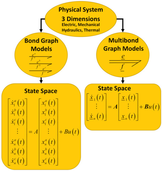
Figure 1. Comparison between bond graphs and multibond graphs.

The following papers related to multibond graphs can be cited: The multibond graph notation becomes a direct way to represent the behavior of energy, power, and other physical properties of multiport systems, which was introduced in [21]. The causality assignment of vector bond graphs was proposed in [24]. The bond graph description of rigid body rotation was described in [25]. Some equivalent procedures for junction structures with gyrators were shown in [26]. Multiport resistors, storage elements, transformers, and gyrators can be decomposed into 1- and 2-port elements, which was proposed in [27]. In [28], it was proven that a bond graph with the junction structure and the mathematical representation corresponds to a port-Hamiltonian system. The representation of the real and imaginary part of the phasors for electrical circuits using multibond graphs was presented in [29]. The linearization of a class of non-linear systems represented by multibond graphs was proposed in [30]. In [31], a pseudo bond graph of a greenhouse was elaborated to simulate temperature and relative humidity inside using multiport (three ports) elements to describe the state of a two element (dry air and water vapor) fluid.

Some recent papers with multibond graphs are as follows: A bond graph model of a helicopter’ssemi-active suspension and the associated simulations were proposed in [32]. The application of a three-dimensional multi-body bond graph modeling approach for simulating vibration in a horizontal oil well was presented in [33]. In [34], a method for an explicit port-Hamiltonian formulation of multibond graphs was introduced.

In this paper, a direct methodology to obtain the steady state of linear time invariant (LTI) systems modeled by multibond graphs is presented. First, Lemma 1 establishes the multiport junction structure of a multibond graph in an integral causality assignment (MBGI) whose multiport storage elements can have integral and derivative causality assignments. From this MBGI, the state space of this system is obtained. With the advantages of the causality of a system in the physical domain, a multibond graph in a derivative causality assignment (MBGD) is proposed. Based on this MBGD, a theorem to obtain the steady state of the state variables of the system is proposed.

Classical methods for determining the steady state to determine the start of the model of the multibody system are described by differential equations [35], state space, or transfer matrices [36]. However, the methodology proposed in this paper allows modeling and determining the structural properties of the multibody system without requiring its mathematical model. Furthermore, the inversion of the state matrix for multiport systems is carried out with the change of causality.

The main contribution of this paper is to obtain the steady state response of an LTI stable system when the state matrix $\left(\mathbf{A}\right)$ is invertible in a multibond graph approach. When this system is modeled by an MBGI, the representation in state space $\left(\mathbf{A},\mathbf{B},\mathbf{C},\mathbf{D}\right)$ can be calculated, and the dynamic and steady state responses during a simulation process are shown. The inverse of the state matrix $\left({\mathbf{A}}^{-1}\right)$ to get the mathematical description of the steady state using an MBGI is required. However, if the corresponding MBGD of this system is obtained, the steady state in a direct way is determined. This result requires calculating the matrix that relates the inputs of the system with the state variables $\left({\mathbf{B}}^{\ast }\right)$ and the outputs of the system $\left({\mathbf{D}}^{\ast }\right)$ where $\left({\mathbf{B}}^{\ast }=-{\mathbf{A}}^{-1}\mathbf{B}\right)$ and $\left({\mathbf{D}}^{\ast }=\mathbf{D}-{\mathbf{CA}}^{-1}\mathbf{B}\right)$. Hence, the steady state for the state $\left(\underline{x_{ss}}\right)$ and output $\left(\underline{y_{ss}}\right)$ variables is defined by $\underline{x_{ss}}=B^{\ast }\underline{u_{ss}}$ and $y_{ss}=D^{\ast }\underline{u_{ss}}$, respectively, where $\underline{u_{ss}}$ is the steady state for the system inputs. Therefore, the change from integral to derivative causality determines the inversion of the state matrix.

The great advantage of this paper with respect to the traditional algebraic approach is that the steady state can be obtained without the need for the mathematical model in the state space of the system. The matrices $B^{\ast }$ and $D^{\ast }$ that determine the steady state are obtained in a direct way from the MBGD. Furthermore, the inverse of the state matrix is not required, which is shown in Figure 2.

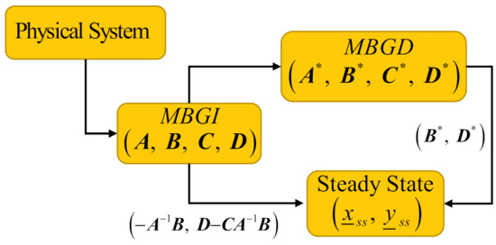
Figure 2. Steady state comparison via a multibond graph in an integral causality assignment (MBGI) and the traditional approach. MBGD, multibond graph in a derivative causality.

References [21,22,23,24,25,26,27,28,29,30,31] used multibond graphs for the modeling and simulation of systems without requiring the calculation of the steady state response. Furthermore, References [32,33] modeled and simulated multibody systems using multibond graphs. However, a comparison of this paper with these references cannot be made. Moreover, the systems of these references can be case studies for the determination of the steady state response, as long as these systems have the conditions required by this paper.

Given a system, it is desired that all the storage elements have integral causality because derivative causality determines linear dependence. However, derivative causality to obtain the properties of structural controllability and structural observability has been used. In this paper, determining the steady state behavior is applied. Derivative causality allows changing the inputs and outputs of the storage elements that result in interesting properties of the systems. For example, in [37,38], the invertibility of the state matrix of an LTI system was obtained. In [39], the mixture of the integral and derivative causality for a singularly perturbed LTI system determined the quasi-steady state model.

The advantage of this approach is the symbolic determination of the steady state response, and this result can be useful for the analysis or synthesis of systems. Mainly multibond graphs have been used for modeling, and the motivation to develop this paper is to link many procedures and tools for single bond graphs to multibond graphs. Hence, the results given in this paper can be extended to a class of non-linear systems.

Section 2 describes the typical modeling in bond graphs. The multiport junction structure of an MBGI is proposed in Section 3. By assigning a derivative causality to the multiport storage elements, the multiport junction structure of an MBGD is introduced in Section 4. The main result of this paper (steady state) is presented in this section. The proposed methodology is applied to two case studies. A three-phase electrical system modeled by a multibond graph is proposed. Hence, the steady state of the electrical currents is obtained. The synchronous generator modeled by a multibond graph is the other case study. The corresponding MBGDs of the generator and steady state are obtained. Simulation results to verify this approach are shown. Finally, Section 5 gives the conclusions.

2. Modeling in a Bond Graph

The connection of two components always determines the power interactions. Furthermore, power can flow in any direction. In the bond graph methodology, effort e and flow f are denoted as the power variables. The product of these variables represents the power P flowing into or out of a port. The representation of a bond is shown in Figure 3 [40,41].

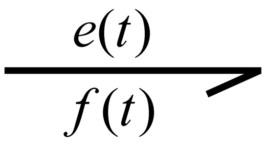
Figure 3. Power bond.

The power variables for some physical systems are indicated in Table 1.

Table 1. Power variables.

System	Effort $\left(\mathit{e}\right)$	Flow $\left(\mathit{f}\right)$
Mechanical	Force $\left(F\right)$	Ang.velocity $\left(\omega \right)$
	Torque $\left(\tau \right)$	Velocity $\left(\nu \right)$
Electrical	Voltage $\left(v\right)$	Current $\left(i\right)$
Hydraulic	Pressure $\left(P\right)$	Volume flow rate $\left(Q\right)$

Furthermore, the energy variables are necessary, denoted by momentum $p\left(t\right)$ and displacement $q\left(t\right)$ where $p\left(t\right)=\int e\left(t\right)dt$ and $q\left(t\right)=\int f\left(t\right)dt$. At each port, both an effort and a flow exist. If one of the effort or flow variables is an input, the other will be the output. The relationship is called causality. Hence, effort and flow are in opposite directions. The causal stroke is represented by a short and perpendicular line made at one end of a bond. The direction of the effort variable is indicated by the causal stroke, as shown in Figure 4 [40,41].

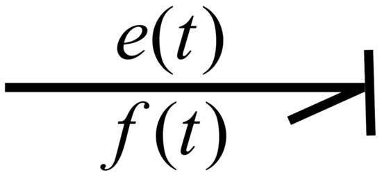
Figure 4. Causal bond.

Moreover, the sources, dissipation, and storage elements can be modeled in the bond graph, and Table 2 gives these elements with their causal relations.

Table 2. Causal forms for one-ports.

Element	Causal Form	Causal Relation
Effort Source		$e\left(t\right)=E\left(t\right)$
Flow Source		$f\left(t\right)=F\left(t\right)$
Resistance		$e\left(t\right)={\Phi }_R\left(f\left(t\right)\right)$ $f\left(t\right)={\Phi }_R^{-1}\left(e\left(t\right)\right)$
Capacitance		$e\left(t\right)={\Phi }_C(\int f\left(t\right)dt)$ $f\left(t\right)={\Phi }_C^{-1}\left(\frac{de\left(t\right)}{dt}\right)$
Inertia		$e\left(t\right)={\Phi }_I(\int e\left(t\right)dt)$ $f\left(t\right)={\Phi }_I^{-1}\left(\frac{df\left(t\right)}{dt}\right)$

The basic elements of the multibond graphs are described in the next section.

3. A Multibond Graph in an Integral Causality Assignment

In a multibond graph, the power variables are denoted by $\underline{e}\left(t\right)$ and $\underline{f}\left(t\right)$, where an array of efforts or flows is given by an underscore. The typical single bond and a multibond are shown in Figure 5 [15].

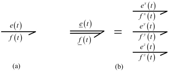
Figure 5. Bonds; (a) single bond; (b) multibond.

Then, the composition of bonds results in a multibond according to Figure 3. The multibond corresponds to three axes $\left(x,y,z\right)$, and the power variables are given by:

$$\underline{e}\left(t\right)=\left[\begin{array}{c}{e}^x\left(t\right)\\ e^y\left(t\right)\\ e^z\left(t\right)\end{array}\right];\underline{f}\left(t\right)=\left[\begin{array}{c}{f}^x\left(t\right)\\ f^y\left(t\right)\\ f^z\left(t\right)\end{array}\right]$$

The power in any multibond is defined by $P\left(t\right)={\underline{e}}^T\left(t\right)\underline{f}\left(t\right)$, where ${\underline{e}}^T\left(t\right)$ is the transpose of $\underline{e}\left(t\right)$. To express that the symbols, “1” and “0” represent arrays of 1-junctions and 0-junctions, respectively; they are given by underscores. Then, the junctions in a multibond graph are $\left(\underline{1},\underline{0}\right)$. A basic multibond graph showing power variables, general multiport elements represented by $MP$, and junctions is illustrated in Figure 6.

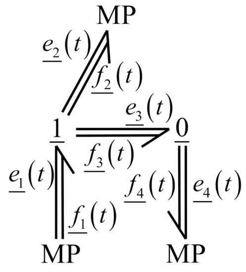
Figure 6. Multibond graph with efforts and flows.

Furthermore, a multibond graph model is constructed of multiport elements, which can be multiport storage elements $\left(\mathbb{C},\mathbb{I}\right)$, multiport dissipation elements $\mathbb{R}$, and/or multiport sources $\left(\underline{M{S}_e},\underline{M{S}_f}\right)$. These elements are shown in Figure 7 [15].

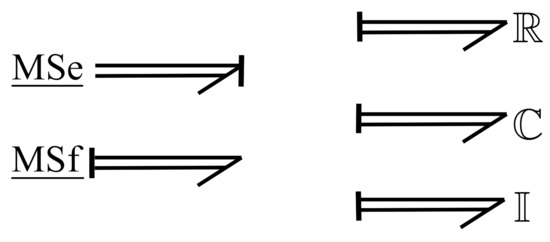
Figure 7. Multiport elements.

Multiport gyrators are essential elements in some multibond graph models that determine the Eulerian junction structure, as shown in Figure 8 [15]. This multiport gyrator is the triangle structure of three one-junctions and three gyrators, internally modulated by the opposite junctions, which represent the gyroscopic forces described by the exterior product in Euler’s equations for rotating coordinate frames.

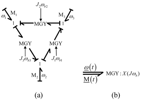
Figure 8. Eulerian junction structure: (a) Euler ring; (b) multiport gyrator.

The corresponding constitutive relationship of the multiport gyrator is defined by:

$$\begin{array}{ccc}\hfill \underline{M}\left(t\right)& =& \left[\begin{array}{c}{M}_1\left(t\right)\\ M_2\left(t\right)\\ M_3\left(t\right)\end{array}\right]=X\left(J{w}_b\right)\underline{w}\left(t\right)\hfill \\ & =& \left[\begin{array}{ccc}0& J_3{w}_{b3}& -J_2{w}_{b2}\\ -J_3{w}_{b3}& 0& J_1{w}_{b1}\\ J_2{w}_{b2}& -J_1{w}_{b1}& 0\end{array}\right]\left[\begin{array}{c}{w}_1\left(t\right)\\ w_2\left(t\right)\\ w_3\left(t\right)\end{array}\right]\hfill \end{array}$$

where $w_b={\left[\begin{array}{ccc}{w}_{b1}& w_{b2}& w_{b3}\end{array}\right]}^T$ is constant for this paper.

The different multiport elements that are part of a multibond graph model can be grouped into interconnected blocks. Therefore, a multiport system represented by a multibond graph model in a predefined integral causality assignment (MBGI) and their key vectors are shown in Figure 9.

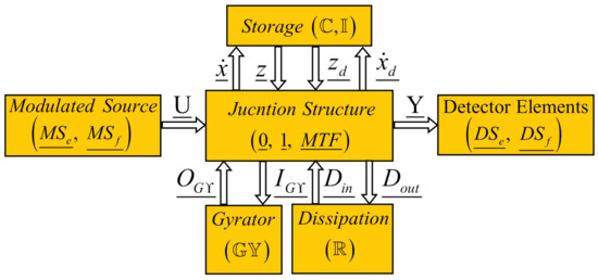
Figure 9. Junction structure and key vectors of a multibond graph with integral causality assignment.

The multiport elements of Figure 7 are as follows:

• $\left(\underline{M{S}_e},\underline{M{S}_f}\right)$ represent the effort and flow modulated multiport sources.
• $\left(\mathbb{C},\mathbb{I}\right)$ denote the multiport storage elements defined by multiport capacitance and inertia, respectively.
• $\mathbb{R}$ are the multiport dissipation elements that constitute the multiport resistors.
• $\left(\underline{0},\underline{1},\underline{MTF}\right)$ represent the multiport junction structure with $\underline{0}$ and $\underline{1}$ multiport junctions, and the multiport transformers are denoted by $\underline{MTF}$.
• $\mathbb{GY}$ is the multiport gyrator.
• $\left(\underline{D{S}_e},\underline{D{S}_f}\right)$ determine the detectors for the effort and flow, respectively.

The multiport energy variables are $\underline{p}\left(t\right)$ and $\underline{q}\left(t\right)$ related to multiport elements $\mathbb{I}$ and $\mathbb{C}$, respectively. The key vectors in Figure 7 are as follows:

• $\underline{x}\left(t\right)\in {\Re }^{\underline{n}}$ and $\underline{x_d}\left(t\right)\in {\Re }^{\underline{m}}$ represent the multiport state variables for multiport storage elements in integral and derivative causality assignments, respectively.
• $\underline{z}\left(t\right)\in {\Re }^{\underline{n}}$ and $\underline{z_d}\left(t\right)\in {\Re }^{\underline{m}}$ are the co-energy vectors for multiport storage elements in integral and derivative causality assignments, respectively.
• $\underline{I_{GY}}\left(t\right)\in {\Re }^{\underline{s}}$ and $\underline{O_{GY}}\left(t\right)\in {\Re }^{\underline{s}}$ denote the inputs and outputs of the multiport gyrators.
• $\underline{D_{in}}\left(t\right)\in {\Re }^{\underline{r}}$ and $\underline{D_{out}}\left(t\right)\in {\Re }^{\underline{r}}$ represent the relationships between the multiport junction structure and multiport dissipation elements.
• $\underline{u}\left(t\right)\in {\Re }^{\underline{p}}$ and $\underline{y}\left(t\right)\in {\Re }^{\underline{q}}$ determine the multiport inputs and outputs of the system.

The state space representation of a multiport system based on a multibond graph model is described by the following Lemma:

Lemma 1.

Consider an LTI system modeled by a multibond graph with a preferred integral causality assignment (MBGI) whose multiport storage elements can have integral and derivative causality assignments. The relationships of the multiport key vectors are shown in Figure 9, and the multiport junction structure is determined by:

$$\left[\begin{array}{c}\stackrel{•}{\underline{x}}\left(t\right)\\ \underline{I_{GY}}\left(t\right)\\ \underline{D_{in}}\left(t\right)\\ \underline{y}\left(t\right)\\ \underline{z_d}\left(t\right)\end{array}\right]=\left[\begin{array}{ccccc}{\mathbf{S}}_{11}^{11}& {\mathbf{S}}_{11}^{12}& {\mathbf{S}}_{12}^{11}& {\mathbf{S}}_{13}^{11}& {\mathbf{S}}_{14}^{11}\\ {\mathbf{S}}_{11}^{21}& {\mathbf{S}}_{11}^{22}& {\mathbf{S}}_{12}^{21}& {\mathbf{S}}_{13}^{21}& \mathbf{0}\\ {\mathbf{S}}_{21}^{11}& {\mathbf{S}}_{21}^{12}& {\mathbf{S}}_{22}& {\mathbf{S}}_{23}& \mathbf{0}\\ {\mathbf{S}}_{31}^{11}& {\mathbf{S}}_{31}^{12}& {\mathbf{S}}_{32}& {\mathbf{S}}_{33}& \mathbf{0}\\ {\mathbf{S}}_{41}^{11}& \mathbf{0}& \mathbf{0}& \mathbf{0}& \mathbf{0}\end{array}\right]\left[\begin{array}{c}\underline{z}\left(t\right)\\ \underline{O_{GY}}\left(t\right)\\ \underline{D_{out}}\left(t\right)\\ \underline{u}\left(t\right)\\ \underline{{\stackrel{•}{x}}_d}\left(t\right)\end{array}\right]$$

(1)

where the entries of $\mathbf{S}$ take values inside the set $\left\{\mathbf{0},\pm \mathbf{I},\pm {\mathbf{K}}_t\right\}$, $\mathbf{I}$ being the identity matrix and ${\mathbf{K}}_t$ the multiport transformer module. The constitutive relationships for the multiport elements are given by:

$$\begin{array}{ccc}\hfill \underline{z}\left(t\right)& =& \mathbf{F}\underline{x}\left(t\right)\hfill \end{array}$$

(2)

$$\begin{array}{ccc}\hfill \underline{z_d}\left(t\right)& =& {\mathbf{F}}_d\underline{x_d}\left(t\right)\hfill \end{array}$$

(3)

$$\begin{array}{ccc}\hfill \underline{O_{GY}}\left(t\right)& =& {\mathbf{X}}_{GY}\underline{I_{GY}}\left(t\right)\hfill \end{array}$$

(4)

$$\begin{array}{ccc}\hfill \underline{D_{out}}\left(t\right)& =& \mathbf{L}\underline{D_{in}}\left(t\right)\hfill \end{array}$$

(5)

Furthermore, the properties of the submatrices of S are: (1) $S_{11}^{11}$, $S_{11}^{22}$, and $S_{22}$ are skew-symmetric; (2) $S_{11}^{12}=-{\left({\mathbf{S}}_{11}^{21}\right)}^T,$ $S_{12}^{11}=-{\left({\mathbf{S}}_{21}^{11}\right)}^T,$$S_{14}^{11}=-{\left({\mathbf{S}}_{41}^{11}\right)}^T$, and ${\mathbf{S}}_{12}^{21}=-{\left({\mathbf{S}}_{21}^{12}\right)}^T$, then a state space representation of the multiport system is defined by:

$$\left[\begin{array}{c}\stackrel{•}{\underline{x}}\left(t\right)\\ \underline{y}\left(t\right)\end{array}\right]=\left[\begin{array}{cc}\mathbf{A}& \mathbf{B}\\ \mathbf{C}& \mathbf{D}\end{array}\right]\left[\begin{array}{c}\underline{x}\left(t\right)\\ \underline{u}\left(t\right)\end{array}\right]$$

(6)

where the corresponding matrices are:

$$\begin{array}{ccc}\hfill \mathbf{A}& =& {\mathbf{E}}^{-1}\left[{\mathbf{S}}_{11}^{11}+{\mathbf{S}}_{11}^{12}{\mathbf{Q}}_X{\mathbf{S}}_{XA}+{\mathbf{S}}_{12}^{11}{\mathbf{Q}}_L{\mathbf{S}}_{LA}\right]\mathbf{F}\hfill \end{array}$$

(7)

$$\begin{array}{ccc}\hfill \mathbf{B}& =& {\mathbf{E}}^{-1}\left[{\mathbf{S}}_{13}^{11}+{\mathbf{S}}_{11}^{12}{\mathbf{Q}}_X{\mathbf{S}}_{XB}+{\mathbf{S}}_{12}^{11}{\mathbf{Q}}_L{\mathbf{S}}_{LB}\right]\hfill \end{array}$$

(8)

$$\begin{array}{ccc}\hfill \mathbf{C}& =& \left[{\mathbf{S}}_{31}^{11}+{\mathbf{S}}_{31}^{12}{\mathbf{Q}}_X{\mathbf{S}}_{XA}+{\mathbf{S}}_{32}{\mathbf{Q}}_L{\mathbf{S}}_{LA}\right]\mathbf{F}\hfill \end{array}$$

(9)

$$\begin{array}{ccc}\hfill \mathbf{D}& =& {\mathbf{S}}_{33}+{\mathbf{S}}_{31}^{12}{\mathbf{Q}}_X{\mathbf{S}}_{XB}+{\mathbf{S}}_{32}{\mathbf{Q}}_L{\mathbf{S}}_{LB}\hfill \end{array}$$

(10)

with:

$$\mathbf{E}=\mathbf{I}-{\mathbf{S}}_{14}^{11}{\mathbf{F}}_d^{-1}{\mathbf{S}}_{41}^{11}\mathbf{F}$$

(11)

and the algebraic loops matrices are described by:

$$\begin{array}{ccc}\hfill {\mathbf{Q}}_X& =& {\mathbf{X}}_{GY}{\left[\mathbf{I}-\left({\mathbf{S}}_{11}^{22}+{\mathbf{S}}_{12}^{21}{\mathbf{M}}_L{\mathbf{S}}_{21}^{12}\right){\mathbf{X}}_{GY}\right]}^{-1}\hfill \end{array}$$

(12)

$$\begin{array}{ccc}\hfill {\mathbf{Q}}_L& =& \mathbf{L}{\left[\mathbf{I}-\left({\mathbf{S}}_{22}+{\mathbf{S}}_{21}^{12}{\mathbf{M}}_X{\mathbf{S}}_{12}^{21}\right)\mathbf{L}\right]}^{-1}\hfill \end{array}$$

(13)

$$\begin{array}{ccc}\hfill {\mathbf{M}}_X& =& {\mathbf{X}}_{GY}{\left(\mathbf{I}-{\mathbf{S}}_{11}^{22}{\mathbf{X}}_{GY}\right)}^{-1}\hfill \end{array}$$

(14)

$$\begin{array}{ccc}\hfill {\mathbf{M}}_L& =& \mathbf{L}{\left(\mathbf{I}-{\mathbf{S}}_{22}\mathbf{L}\right)}^{-1}\hfill \end{array}$$

(15)

$$\begin{array}{ccc}\hfill {\mathbf{S}}_{XA}& =& {\mathbf{S}}_{11}^{21}+{\mathbf{S}}_{12}^{21}{\mathbf{M}}_L{\mathbf{S}}_{21}^{11}\hfill \end{array}$$

(16)

$$\begin{array}{ccc}\hfill {\mathbf{S}}_{LA}& =& {\mathbf{S}}_{21}^{11}+{\mathbf{S}}_{21}^{12}{\mathbf{M}}_X{\mathbf{S}}_{11}^{21}\hfill \end{array}$$

(17)

$$\begin{array}{ccc}\hfill {\mathbf{S}}_{XB}& =& {\mathbf{S}}_{13}^{21}+{\mathbf{S}}_{12}^{21}{\mathbf{M}}_L{\mathbf{S}}_{23}\hfill \end{array}$$

(18)

$$\begin{array}{ccc}\hfill {\mathbf{S}}_{LB}& =& {\mathbf{S}}_{23}+{\mathbf{S}}_{21}^{12}{\mathbf{M}}_X{\mathbf{S}}_{13}^{21}\hfill \end{array}$$

(19)

The proof of Lemma 1 is presented in Appendix A.

The state equation described by Lemma 1 determines a system with linearly independent and dependent state variables according to the causality of the multiport storage elements. Hence, matrix $\mathbf{E}$ gives the relationships between these state variables.

When the dynamic period of a stable system has finished, the steady state response can be obtained. From (6) and setting $\stackrel{•}{\underline{x}}\left(t\right)=0$ for a system with invertible state matrix $\mathbf{A}$, the steady state is defined by:

$$\begin{array}{ccc}\hfill \underline{x_{ss}}& =& -{\mathbf{A}}^{-1}\mathbf{B}\underline{u_{ss}}\hfill \end{array}$$

(20)

$$\begin{array}{ccc}\hfill \underline{y_{ss}}& =& \left(\mathbf{D}-{\mathbf{CA}}^{-1}\mathbf{B}\right)\underline{u_{ss}}\hfill \end{array}$$

(21)

where $\underline{x_{ss}},$$\underline{y_{ss}}$ and $\underline{u_{ss}}$ denote the steady state of the state variables, outputs and inputs, respectively.

The steady state response of multiport systems in a multibond graph approach is presented in the next section.

4. A Multibond Graph in a Derivative Causality Assignment

The information on the causality of a bond graph model has been a great tool to find easy and direct results in the physical domain. The assignment of integral causality to a single bond graph (BGI) and a multibond graph (MBGI) can determine the state spaces of the systems. Furthermore, the structural controllability and structural observability of a system in the physical domain are obtained through the causal paths from the sources and detectors to the storage elements, respectively. Hence, the linearization of systems modeled by single bond graphs or multibond graphs using causal paths have been presented [30].

In order to get the steady state of a system, a derivative causality for the multiport storage elements of a multibond graph is assigned (MBGD), which is shown in Figure 10.

Figure 10. Multibond graph in a derivative causality assignment.

Figure 10 illustrates that all the multiport storage elements have a derivative causality assignment, and the multiport dissipation elements and multiport gyrators must have the appropriate causality to get a correct multibond graph model. The relationships of the MBGD are obtained through the following Lemma.

Lemma 2.

Consider a multibond graph model in a preferred derivative causality assignment (MBGD) of an LTI system whose scheme is shown in Figure 10, where all the multiport storage elements have a derivative causality assignment and the multiport junction structure is defined by:

$$\left[\begin{array}{c}\underline{z}\left(t\right)\\ \underline{z_d}\left(t\right)\\ \underline{I_{GY}^d}\left(t\right)\\ \underline{D_{in}^d}\left(t\right)\\ \underline{y}\left(t\right)\end{array}\right]=\left[\begin{array}{ccccc}{\mathbf{J}}_{11}^{11}& {\mathbf{J}}_{11}^{12}& {\mathbf{J}}_{11}^{13}& {\mathbf{J}}_{12}^{11}& {\mathbf{J}}_{13}^{11}\\ {\mathbf{J}}_{11}^{21}& {\mathbf{J}}_{11}^{22}& {\mathbf{J}}_{11}^{23}& {\mathbf{J}}_{12}^{21}& {\mathbf{J}}_{13}^{21}\\ {\mathbf{J}}_{11}^{31}& {\mathbf{J}}_{11}^{32}& {\mathbf{J}}_{11}^{33}& {\mathbf{J}}_{12}^{31}& {\mathbf{J}}_{13}^{31}\\ {\mathbf{J}}_{21}^{11}& {\mathbf{J}}_{21}^{12}& {\mathbf{J}}_{21}^{13}& {\mathbf{J}}_{22}& {\mathbf{J}}_{23}\\ {\mathbf{J}}_{31}^{11}& {\mathbf{J}}_{31}^{12}& {\mathbf{J}}_{31}^{13}& {\mathbf{J}}_{32}& {\mathbf{J}}_{33}\end{array}\right]\left[\begin{array}{c}\stackrel{•}{\underline{x}}\left(t\right)\\ \underline{\stackrel{•}{x_d}}\left(t\right)\\ \underline{O_{GY}^d}\left(t\right)\\ \underline{D_{out}^d}\left(t\right)\\ \underline{u}\left(t\right)\end{array}\right]$$

(22)

where the entries of $\mathbf{J}$ take values inside the set $\left\{\mathbf{0},\pm \mathbf{I},\pm {\mathbf{K}}_t\right\}$, $\mathbf{I}$ being the identity matrix and ${\mathbf{K}}_t$ the multiport transformer module. The constitutive relations for the multiport dissipation and multiport gyrators are expressed by:

$$\begin{array}{ccc}\hfill \underline{D_{out}^d}\left(t\right)& =& {\mathbf{L}}^d\underline{D_{in}^d}\left(t\right)\hfill \end{array}$$

(23)

$$\begin{array}{ccc}\hfill \underline{O_{GY}^d}\left(t\right)& =& {\mathbf{X}}_{GY}^d\underline{I_{GY}^d}\left(t\right)\hfill \end{array}$$

(24)

The multiport storage elements are given by (2) and (3). Furthermore, the properties of the submatrices of $\mathbf{J}$ are: (1) ${\mathbf{J}}_{11}^{11}$, ${\mathbf{J}}_{11}^{22}$, ${\mathbf{J}}_{11}^{33}$, and ${\mathbf{J}}_{22}$ are skew-symmetric; (2) ${\mathbf{J}}_{11}^{12}=-{\left({\mathbf{J}}_{11}^{21}\right)}^T,$ ${\mathbf{J}}_{11}^{13}=-{\left({\mathbf{J}}_{11}^{31}\right)}^T,$ ${\mathbf{J}}_{12}^{11}=-{\left({\mathbf{J}}_{21}^{11}\right)}^T,$ ${\mathbf{J}}_{11}^{23}=-{\left({\mathbf{J}}_{11}^{32}\right)}^T,$ ${\mathbf{J}}_{12}^{21}=-{\left({\mathbf{J}}_{21}^{12}\right)}^T$, and ${\mathbf{J}}_{12}^{31}=-{\left({\mathbf{J}}_{21}^{13}\right)}^T$. A state space representation of this multiport system is described by:

$$\left[\begin{array}{c}\underline{x}\left(t\right)\\ \underline{x_d}\left(t\right)\\ \underline{y}\left(t\right)\end{array}\right]=\left[\begin{array}{cc}{\mathbf{A}}_{11}^{\ast }& {\mathbf{A}}_{12}^{\ast }\\ {\mathbf{A}}_{21}^{\ast }& {\mathbf{A}}_{22}^{\ast }\\ {\mathbf{C}}^{\ast }& {\mathbf{G}}^{\ast }\end{array}\right]\left[\begin{array}{c}\stackrel{•}{\underline{x}}\left(t\right)\\ \underline{\stackrel{•}{x_d}}\left(t\right)\end{array}\right]+\left[\begin{array}{c}{\mathbf{B}}_1^{\ast }\\ {\mathbf{B}}_2^{\ast }\\ {\mathbf{D}}^{\ast }\end{array}\right]\underline{u}\left(t\right)$$

(25)

where the matrix partition is given by:

$$\begin{array}{ccc}\hfill {\mathbf{A}}_{11}^{\ast }& =& {\mathbf{F}}^{-1}\left[{\mathbf{J}}_{11}^{11}+{\mathbf{J}}_{11}^{13}{\mathbf{P}}_X{\mathbf{J}}_{XA}^{11}+{\mathbf{J}}_{12}^{11}{\mathbf{P}}_L{\mathbf{J}}_{LA}^{11}\right]\hfill \end{array}$$

(26)

$$\begin{array}{ccc}\hfill {\mathbf{A}}_{12}^{\ast }& =& {\mathbf{F}}^{-1}\left[{\mathbf{J}}_{11}^{12}+{\mathbf{J}}_{11}^{13}{\mathbf{P}}_X{\mathbf{J}}_{XA}^{12}+{\mathbf{J}}_{12}^{11}{\mathbf{P}}_L{\mathbf{J}}_{LA}^{12}\right]\hfill \end{array}$$

(27)

$$\begin{array}{ccc}\hfill {\mathbf{A}}_{21}^{\ast }& =& {\mathbf{F}}_d^{-1}\left[{\mathbf{J}}_{11}^{21}+{\mathbf{J}}_{11}^{23}{\mathbf{P}}_X{\mathbf{J}}_{XA}^{11}+{\mathbf{J}}_{12}^{21}{\mathbf{P}}_L{\mathbf{J}}_{LA}^{11}\right]\hfill \end{array}$$

(28)

$$\begin{array}{ccc}\hfill {\mathbf{A}}_{22}^{\ast }& =& {\mathbf{F}}_d^{-1}\left[{\mathbf{J}}_{11}^{22}+{\mathbf{J}}_{11}^{23}{\mathbf{P}}_X{\mathbf{J}}_{XA}^{12}+{\mathbf{J}}_{12}^{21}{\mathbf{P}}_L{\mathbf{J}}_{LA}^{12}\right]\hfill \end{array}$$

(29)

$$\begin{array}{ccc}\hfill {\mathbf{B}}_1^{\ast }& =& {\mathbf{F}}^{-1}\left[{\mathbf{J}}_{13}^{11}+{\mathbf{J}}_{11}^{13}{\mathbf{P}}_X{\mathbf{J}}_{XB}+{\mathbf{J}}_{12}^{11}{\mathbf{P}}_L{\mathbf{J}}_{LB}\right]\hfill \end{array}$$

(30)

$$\begin{array}{ccc}\hfill {\mathbf{B}}_2^{\ast }& =& {\mathbf{F}}_d^{-1}\left[{\mathbf{J}}_{13}^{21}+{\mathbf{J}}_{11}^{23}{\mathbf{P}}_X{\mathbf{J}}_{XB}+{\mathbf{J}}_{12}^{21}{\mathbf{P}}_L{\mathbf{J}}_{LB}\right]\hfill \end{array}$$

(31)

and the corresponding matrices for the output are:

$$\begin{array}{ccc}\hfill {\mathbf{C}}^{\ast }& =& {\mathbf{J}}_{31}^{11}+{\mathbf{J}}_{21}^{13}{\mathbf{P}}_X{\mathbf{J}}_{XA}^{11}+{\mathbf{J}}_{32}{\mathbf{P}}_L{\mathbf{J}}_{LA}^{11}\hfill \end{array}$$

(32)

$$\begin{array}{ccc}\hfill {\mathbf{G}}^{\ast }& =& {\mathbf{J}}_{31}^{12}+{\mathbf{J}}_{21}^{13}{\mathbf{P}}_X{\mathbf{J}}_{XA}^{12}+{\mathbf{J}}_{32}{\mathbf{P}}_L{\mathbf{J}}_{LA}^{12}\hfill \end{array}$$

(33)

$$\begin{array}{ccc}\hfill {\mathbf{D}}^{\ast }& =& {\mathbf{J}}_{33}+{\mathbf{J}}_{21}^{13}{\mathbf{P}}_X{\mathbf{J}}_{XB}+{\mathbf{J}}_{32}{\mathbf{P}}_L{\mathbf{J}}_{LB}\hfill \end{array}$$

(34)

with:

$$\begin{array}{ccc}\hfill {\mathbf{J}}_{XA}^{11}& =& {\mathbf{J}}_{11}^{31}+{\mathbf{J}}_{12}^{31}{\mathbf{N}}_L{\mathbf{J}}_{21}^{11}\hfill \end{array}$$

(35)

$$\begin{array}{ccc}\hfill {\mathbf{J}}_{LA}^{11}& =& {\mathbf{J}}_{21}^{11}+{\mathbf{J}}_{21}^{13}{\mathbf{N}}_X{\mathbf{J}}_{11}^{31}\hfill \end{array}$$

(36)

$$\begin{array}{ccc}\hfill {\mathbf{J}}_{XA}^{12}& =& {\mathbf{J}}_{11}^{32}+{\mathbf{J}}_{21}^{31}{\mathbf{N}}_L{\mathbf{J}}_{21}^{12}\hfill \end{array}$$

(37)

$$\begin{array}{ccc}\hfill {\mathbf{J}}_{LA}^{12}& =& {\mathbf{J}}_{21}^{12}+{\mathbf{J}}_{21}^{13}{\mathbf{N}}_X{\mathbf{J}}_{11}^{32}\hfill \end{array}$$

(38)

$$\begin{array}{ccc}\hfill {\mathbf{J}}_{XB}& =& {\mathbf{J}}_{13}^{31}+{\mathbf{J}}_{12}^{31}{\mathbf{N}}_L{\mathbf{J}}_{23}\hfill \end{array}$$

(39)

$$\begin{array}{ccc}\hfill {\mathbf{J}}_{LB}& =& {\mathbf{J}}_{23}+{\mathbf{J}}_{21}^{13}{\mathbf{N}}_X{\mathbf{J}}_{13}^{31}\hfill \end{array}$$

(40)

The algebraic loop matrices are:

$$\begin{array}{ccc}\hfill {\mathbf{N}}_L& =& {\mathbf{L}}^d{\left(\mathbf{I}-{\mathbf{J}}_{22}{\mathbf{L}}^d\right)}^{-1}\hfill \end{array}$$

(41)

$$\begin{array}{ccc}\hfill {\mathbf{N}}_X& =& {\mathbf{X}}_{GY}^d{\left(\mathbf{I}-{\mathbf{J}}_{11}^{22}{\mathbf{X}}_{GY}^d\right)}^{-1}\hfill \end{array}$$

(42)

$$\begin{array}{ccc}\hfill {\mathbf{P}}_L& =& {\mathbf{L}}^d{\left(\mathbf{I}-{\mathbf{J}}_{22}{\mathbf{L}}^d-{\mathbf{J}}_{21}^{12}{\mathbf{N}}_X{\mathbf{J}}_{12}^{21}{\mathbf{L}}^d\right)}^{-1}\hfill \end{array}$$

(43)

$$\begin{array}{ccc}\hfill {\mathbf{P}}_X& =& {\mathbf{X}}_{GY}^d{\left(\mathbf{I}-{\mathbf{J}}_{11}^{22}{\mathbf{X}}_{GY}^d-{\mathbf{J}}_{12}^{21}{\mathbf{N}}_L{\mathbf{J}}_{21}^{12}{\mathbf{X}}_{GY}^d\right)}^{-1}\hfill \end{array}$$

(44)

The proof of Lemma 1 is presented in Appendix B.

Based on the multibond graph in a derivative causality assignment of an LTI system, the steady state in the physical domain is proposed in the following Theorem.

Theorem 1.

The steady state of the multiport state variables of multiport LTI stable systems modeled by a multibond graph with a preferred integral causality assignment whose multiport storage elements can have integral and derivative causality assignments and the corresponding multibond graph in a derivative causality assignment has all the multiport storage elements is defined by:

$$\begin{array}{ccc}\hfill \underline{x_{ss}}& =& {\mathbf{B}}^{\ast }\underline{u_{ss}}\hfill \end{array}$$

(45)

$$\begin{array}{ccc}\hfill \underline{y_{ss}}& =& {\mathbf{D}}^{\ast }\underline{u_{ss}}\hfill \end{array}$$

(46)

The proof of Theorem is presented in Appendix C.

Thus, given an MBGI of an LTI system and obtaining the MBGD, the steady state can be determined in a direct way, and it is not necessary to get the state space of the system.

The proposed methodology is applied to the cases study in the next section.

5. Case Study

The multibond graph models for two linear physical systems are analyzed. The steady state behavior of these systems in the physical domain applying the proposed results is presented.

5.1. Three-Phase Electrical System

A three-phase electrical system formed by two sources and a transmission line for each phase is shown in Figure 11.

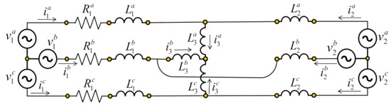
Figure 11. Three-phase electrical system.

Park’s transformation offers a great reduction in the mathematical modeling of three-phase systems. This Parktransformation changes the parameters and variables from phases $\left(a,b,c\right)$ to new variables of the reference frame [42,43]. The new variables are $\left(d,q,0\right)$ with d and q axis components, and a stationary current that is the zero-sequence current is the third variable. Thus, by definition:

$$\left[\begin{array}{c}{i}_d\left(t\right)\\ i_q\left(t\right)\\ i_0\left(t\right)\end{array}\right]=\sqrt{\frac{2}{3}}\left[\begin{array}{ccc}cos\theta & cos\left(\theta -\frac{2\pi }{3}\right)& cos\left(\theta +\frac{2\pi }{3}\right)\\ sin\pi & sin\left(\theta -\frac{2\pi }{3}\right)& sin\left(\theta +\frac{2\pi }{3}\right)\\ {\displaystyle \frac{1}{\sqrt{2}}}& {\displaystyle \frac{1}{\sqrt{2}}}& {\displaystyle \frac{1}{\sqrt{2}}}\end{array}\right]\left[\begin{array}{c}{i}_a\left(t\right)\\ i_b\left(t\right)\\ i_c\left(t\right)\end{array}\right]$$

(47)

The angle $\theta$ is given by:

$$\theta =wt+\frac{\pi }{2}$$

(48)

where w denotes the rated angular frequency in rad/s.

In a similar way, to change the voltages and flux linkages:

$$\begin{array}{ccc}\hfill v^{dq0}\left(t\right)& =& \mathbf{P}{v}^{abc}\left(t\right)\hfill \end{array}$$

(49)

$$\begin{array}{ccc}\hfill {\lambda }^{dq0}\left(t\right)& =& \mathbf{P}{\lambda }^{abc}\left(t\right)\hfill \end{array}$$

(50)

By knowing the importance of Park’s transformation for the analysis of three-phase electrical systems, the multibond graph model of this case study is shown in Figure 12. The dynamic model of the system in the $\left(d,q,0\right)$ axis is modeled by a multibond graph. However, the supply voltages to the system are $\left(a,b,c\right)$ and the multiport transformers to convert $\left(a,b,c\right)$ to $\left(d,q,0\right)$ are applied. Furthermore, the three-phase output current by using a multiport transformer with the inverse Parktransformation is obtained.

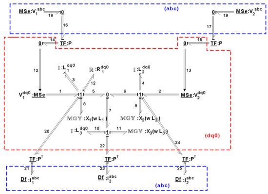
Figure 12. MBGI of the electrical system.

The multiport storage elements in an integral causality assignment are expressed by the following key vectors:

$$\underline{x}\left(t\right)=\left[\begin{array}{c}\underline{p_3}\left(t\right)\\ \underline{p_4}\left(t\right)\end{array}\right];\stackrel{•}{\underline{x}}\left(t\right)=\left[\begin{array}{c}\underline{e_3}\left(t\right)\\ \underline{e_4}\left(t\right)\end{array}\right];\underline{z}\left(t\right)=\left[\begin{array}{c}\underline{f_3}\left(t\right)\\ \underline{f_4}\left(t\right)\end{array}\right]$$

with the constitutive relationship:

$${\mathbf{F}}^{-1}=diag\left\{{\mathbf{L}}_1^{dq0},{\mathbf{L}}_2^{dq0}\right\}$$

(51)

In a derivative causality assignment, they are described by:

$$\underline{x_d}\left(t\right)=\underline{p_{10}}\left(t\right);\stackrel{•}{\underline{x_d}}\left(t\right)=\underline{e_{10}}\left(t\right);\underline{z_d}\left(t\right)=\underline{f_{10}}\left(t\right)$$

with the constitutive relationship:

$${\mathbf{F}}_d^{-1}={\mathbf{L}}_3$$

(52)

The multiport gyrators are defined by:

$$\underline{I_{GY}}\left(t\right)=\left[\begin{array}{c}\underline{f_8}\left(t\right)\\ \underline{f_9}\left(t\right)\\ \underline{f_{11}}\left(t\right)\end{array}\right];\underline{O_{GY}}\left(t\right)=\left[\begin{array}{c}\underline{e_8}\left(t\right)\\ \underline{e_9}\left(t\right)\\ \underline{e_{11}}\left(t\right)\end{array}\right]$$

with:

$${\mathbf{X}}_{GY}=diag\left\{{\mathbf{X}}_1\left(w{L}_1\right),{\mathbf{X}}_2\left(w{L}_2\right),{\mathbf{X}}_3\left(w{L}_3\right)\right\}$$

(53)

For the multiport dissipation elements:

$$\underline{D_{in}}\left(t\right)=\underline{f_{12}}\left(t\right);\underline{D_{out}}\left(t\right)=\underline{e_{12}}\left(t\right)$$

with:

$$\mathbf{L}={\mathbf{R}}_1^{dq0}$$

(54)

and the inputs and outputs are:

$$\underline{u}\left(t\right)=\left[\begin{array}{c}\underline{e_1}\left(t\right)\\ \underline{e_2}\left(t\right)\end{array}\right];\underline{y}\left(t\right)=\left[\begin{array}{c}\underline{f_{21}}\left(t\right)\\ \underline{f_{25}}\left(t\right)\\ \underline{f_{23}}\left(t\right)\end{array}\right]$$

where the matrices for resistors, inductors, and gyrators are:

$$\begin{array}{ccc}\hfill {\mathbf{L}}_i^{dq0}& =& diag\left\{L_i^d,L_i^q,L_i^0\right\};i=1,2,3\hfill \end{array}$$

(55)

$$\begin{array}{ccc}\hfill {\mathbf{R}}_1^{dq0}& =& diag\left\{R_1^d,R_1^q,R_1^0\right\}\hfill \end{array}$$

(56)

$$\begin{array}{ccc}\hfill {\mathbf{X}}_i\left(w{L}_i\right)& =& \left[\begin{array}{ccc}0& w{L}_i^d& 0\\ -w{L}_i^q& 0& 0\\ 0& 0& 0\end{array}\right];i=1,2,3\hfill \end{array}$$

(57)

The multiport junction structure of this MBGI is given by:

$$\left[\begin{array}{c}\underline{e_3}\left(t\right)\\ \underline{e_4}\left(t\right)\\ \underline{f_8}\left(t\right)\\ \underline{f_9}\left(t\right)\\ \underline{f_{11}}\left(t\right)\\ \underline{f_{12}}\left(t\right)\\ \underline{f_{21}}\left(t\right)\\ \underline{f_{25}}\left(t\right)\\ \underline{f_{23}}\left(t\right)\\ \underline{f_{10}}\left(t\right)\end{array}\right]=\left[\begin{array}{ccccccccc}\mathbf{0}& \mathbf{0}& -\mathbf{I}& \mathbf{0}& \mathbf{0}& -\mathbf{I}& \mathbf{I}& \mathbf{0}& -\mathbf{I}\\ \mathbf{0}& \mathbf{0}& \mathbf{0}& -\mathbf{I}& -\mathbf{I}& \mathbf{0}& \mathbf{0}& \mathbf{I}& -\mathbf{I}\\ \mathbf{I}& \mathbf{0}& \mathbf{0}& \mathbf{0}& \mathbf{0}& \mathbf{0}& \mathbf{0}& \mathbf{0}& \mathbf{0}\\ \mathbf{0}& \mathbf{I}& \mathbf{0}& \mathbf{0}& \mathbf{0}& \mathbf{0}& \mathbf{0}& \mathbf{0}& \mathbf{0}\\ \mathbf{I}& \mathbf{I}& \mathbf{0}& \mathbf{0}& \mathbf{0}& \mathbf{0}& \mathbf{0}& \mathbf{0}& \mathbf{0}\\ \mathbf{I}& \mathbf{0}& \mathbf{0}& \mathbf{0}& \mathbf{0}& \mathbf{0}& \mathbf{0}& \mathbf{0}& \mathbf{0}\\ {\mathbf{P}}^T& \mathbf{0}& \mathbf{0}& \mathbf{0}& \mathbf{0}& \mathbf{0}& \mathbf{0}& \mathbf{0}& \mathbf{0}\\ \mathbf{0}& {\mathbf{P}}^T& \mathbf{0}& \mathbf{0}& \mathbf{0}& \mathbf{0}& \mathbf{0}& \mathbf{0}& \mathbf{0}\\ {\mathbf{P}}^T& {\mathbf{P}}^T& \mathbf{0}& \mathbf{0}& \mathbf{0}& \mathbf{0}& \mathbf{0}& \mathbf{0}& \mathbf{0}\\ \mathbf{I}& \mathbf{I}& \mathbf{0}& \mathbf{0}& \mathbf{0}& \mathbf{0}& \mathbf{0}& \mathbf{0}& \mathbf{0}\end{array}\right]\left[\begin{array}{c}\underline{f_3}\left(t\right)\\ \underline{f_4}\left(t\right)\\ \underline{e_8}\left(t\right)\\ \underline{e_9}\left(t\right)\\ \underline{e_{11}}\left(t\right)\\ \underline{e_{12}}\left(t\right)\\ \underline{e_1}\left(t\right)\\ \underline{e_2}\left(t\right)\\ \underline{e_{10}}\left(t\right)\end{array}\right]$$

(58)

In this case,

$${\mathbf{S}}_{11}^{11}={\mathbf{S}}_{11}^{22}={\mathbf{S}}_{22}={\mathbf{S}}_{12}^{21}={\mathbf{S}}_{21}^{12}={\mathbf{S}}_{13}^{21}={\mathbf{S}}_{23}=\mathbf{0}$$

(59)

and (7), (8) are re-written as:

$$\begin{array}{ccc}\hfill \mathbf{A}& =& \left[{\mathbf{S}}_{11}^{12}{\mathbf{X}}_{GY}{\mathbf{S}}_{11}^{21}+{\mathbf{S}}_{12}^{11}{\mathbf{LS}}_{21}^{11}\right]\mathbf{F}\hfill \end{array}$$

(60)

$$\begin{array}{ccc}\hfill \mathbf{B}& =& {\mathbf{S}}_{13}^{11}\hfill \end{array}$$

(61)

From (51, 52, 53, 54,55,56,57,58) with (60) and (61), the state equation of the electrical system is:

$$\begin{array}{ccc}\hfill \mathbf{E}\stackrel{•}{\underline{x}}\left(t\right)& =& -\left[\begin{array}{cc}{\mathbf{R}}_1^{dq0}+{\mathbf{X}}_1\left(w{L}_1\right)+{\mathbf{X}}_3\left(w{L}_3\right)& {\mathbf{X}}_3\left(w{L}_3\right)\\ {\mathbf{X}}_3\left(w{L}_3\right)& {\mathbf{X}}_2\left(w{L}_1\right)+{\mathbf{X}}_3\left(w{L}_3\right)\end{array}\right]{\left[\begin{array}{cc}{\mathbf{L}}_1^{dq0}& \mathbf{0}\\ \mathbf{0}& {\mathbf{L}}_2^{dq0}\end{array}\right]}^{-1}\underline{x}\left(t\right)\hfill \\ & & +\left[\begin{array}{cc}\mathbf{I}& \mathbf{0}\\ \mathbf{0}& \mathbf{I}\end{array}\right]\underline{u}\left(t\right)\hfill \end{array}$$

(62)

where $\mathbf{E}$ is obtained from (11), (51), (52), and (58), which is:

$$\mathbf{E}=\left[\begin{array}{cc}\mathbf{I}+{\mathbf{L}}_3^{dq0}{\left({\mathbf{L}}_1^{dq0}\right)}^{-1}& {\mathbf{L}}_3^{dq0}{\left({\mathbf{L}}_2^{dq0}\right)}^{-1}\\ {\mathbf{L}}_3^{dq0}{\left({\mathbf{L}}_1^{dq0}\right)}^{-1}& \mathbf{I}+{\mathbf{L}}_3^{dq0}{\left({\mathbf{L}}_2^{dq0}\right)}^{-1}\end{array}\right]$$

(63)

with the outputs:

$$\underline{y}\left(t\right)=\left[\begin{array}{cc}{\mathbf{P}}^T& \mathbf{0}\\ \mathbf{0}& {\mathbf{P}}^T\\ {\mathbf{P}}^T& {\mathbf{P}}^T\end{array}\right]{\left[\begin{array}{cc}{\mathbf{L}}_1^{dq0}& \mathbf{0}\\ \mathbf{0}& {\mathbf{L}}_2^{dq0}\end{array}\right]}^{-1}\underline{x}\left(t\right)$$

(64)

When a derivative causality is assigned to the multiport storage elements of a multibond graph, then the corresponding MBGD of the system is shown in Figure 13.

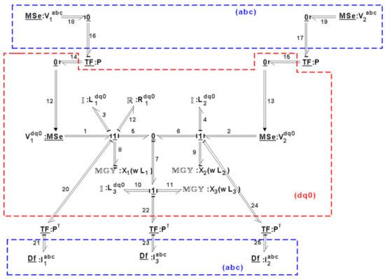
Figure 13. MBGD of the electrical system.

The causality for the two multiport gyrator elements defined by the multibonds 8 and 9 have to be changed in order to have a correct multibond graph, and their key vectors are given by:

$$\underline{I_{GY}^d}\left(t\right)=\left[\begin{array}{c}\underline{e_8}\left(t\right)\\ \underline{e_9}\left(t\right)\\ \underline{f_{11}}\left(t\right)\end{array}\right];\underline{O_{GY}^d}\left(t\right)=\left[\begin{array}{c}\underline{f_8}\left(t\right)\\ \underline{f_9}\left(t\right)\\ \underline{e_{11}}\left(t\right)\end{array}\right]$$

with the constitutive relation:

$${\mathbf{X}}_{GY}^d=diag\left\{{\mathbf{X}}_1^{-1}\left(w{L}_1\right),{\mathbf{X}}_2^{-1}\left(w{L}_2\right),{\mathbf{X}}_3\left(w{L}_3\right)\right\}$$

(65)

and the matrix for the dissipation field is:

$${\mathbf{L}}^d=\mathbf{L}$$

(66)

Now, the multiport junction structure of the MBGD is defined by:

$$\left[\begin{array}{c}\underline{f_3}\left(t\right)\\ \underline{f_4}\left(t\right)\\ \underline{f_{10}}\left(t\right)\\ \underline{e_8}\left(t\right)\\ \underline{e_9}\left(t\right)\\ \underline{f_{11}}\left(t\right)\\ \underline{f_{12}}\left(t\right)\end{array}\right]=\left[\begin{array}{ccccccccc}\mathbf{0}& \mathbf{0}& \mathbf{0}& \mathbf{I}& \mathbf{0}& \mathbf{0}& \mathbf{0}& \mathbf{0}& \mathbf{0}\\ \mathbf{0}& \mathbf{0}& \mathbf{0}& \mathbf{0}& \mathbf{I}& \mathbf{0}& \mathbf{0}& \mathbf{0}& \mathbf{0}\\ \mathbf{0}& \mathbf{0}& \mathbf{0}& \mathbf{I}& \mathbf{I}& \mathbf{0}& \mathbf{0}& \mathbf{0}& \mathbf{0}\\ -\mathbf{I}& \mathbf{0}& -\mathbf{I}& \mathbf{0}& \mathbf{0}& -\mathbf{I}& -\mathbf{I}& \mathbf{I}& \mathbf{0}\\ \mathbf{0}& -\mathbf{I}& -\mathbf{I}& \mathbf{0}& \mathbf{0}& -\mathbf{I}& \mathbf{0}& \mathbf{0}& \mathbf{I}\\ \mathbf{0}& \mathbf{0}& \mathbf{0}& \mathbf{I}& \mathbf{I}& \mathbf{0}& \mathbf{0}& \mathbf{0}& \mathbf{0}\\ \mathbf{0}& \mathbf{0}& \mathbf{0}& \mathbf{I}& \mathbf{0}& \mathbf{0}& \mathbf{0}& \mathbf{0}& \mathbf{0}\end{array}\right]\left[\begin{array}{c}\underline{e_3}\left(t\right)\\ \underline{e_4}\left(t\right)\\ \underline{e_{10}}\left(t\right)\\ \underline{f_8}\left(t\right)\\ \underline{f_9}\left(t\right)\\ \underline{e_{11}}\left(t\right)\\ \underline{e_{12}}\left(t\right)\\ \underline{e_1}\left(t\right)\\ \underline{e_2}\left(t\right)\end{array}\right]$$

(67)

For this case study, from (67), (30) is reduced to:

$${\mathbf{B}}_1^{\ast }={\mathbf{F}}^{-1}{\mathbf{J}}_{11}^{13}{\mathbf{P}}_X{\mathbf{J}}_{13}^{31}$$

(68)

and ${\mathbf{P}}_X$ is re-written as:

$${\mathbf{P}}_X={\mathbf{X}}_{GY}^d{\left(\mathbf{I}-{\mathbf{J}}_{12}^{21}{\mathbf{L}}^d{\mathbf{J}}_{21}^{12}{\mathbf{X}}_{GY}^d\right)}^{-1}$$

(69)

The key step to get the steady state of the system is to calculate (69), which is described in Appendix D.

By substituting (68) into (45) with (67), the steady state response is given by:

$$\underline{x_{ss}}={\mathbf{F}}^{-1}\left[\begin{array}{ccc}\mathbf{I}& \mathbf{0}& \mathbf{0}\\ \mathbf{0}& \mathbf{I}& \mathbf{0}\end{array}\right]{\mathbf{P}}_X\left[\begin{array}{cc}\mathbf{I}& \mathbf{0}\\ \mathbf{0}& \mathbf{I}\\ \mathbf{0}& \mathbf{0}\end{array}\right]\underline{u_{ss}}$$

(70)

Using the co-energy variables as state variables in electrical systems is very common, then from (2) and (70) with (A46):

$$\underline{z_{ss}}=\left[\begin{array}{cc}{P}_{11}^x& P_{12}^x\\ P_{21}^x& P_{22}^x\end{array}\right]\underline{u_{ss}}$$

(71)

The three-phase representation of the system for each state variable is:

$$\begin{array}{ccc}\hfill \underline{p_3}\left(t\right)& =& \left[\begin{array}{c}{p}_3^d\left(t\right)\\ p_3^q\left(t\right)\\ p_3^0\left(t\right)\end{array}\right];\underline{e_3}\left(t\right)=\left[\begin{array}{c}{e}_3^d\left(t\right)\\ e_3^q\left(t\right)\\ e_3^0\left(t\right)\end{array}\right];\underline{f_3}\left(t\right)=\left[\begin{array}{c}{f}_3^d\left(t\right)\\ f_3^q\left(t\right)\\ f_3^0\left(t\right)\end{array}\right]\hfill \\ \hfill \underline{p_4}\left(t\right)& =& \left[\begin{array}{c}{p}_4^d\left(t\right)\\ p_4^q\left(t\right)\\ p_4^0\left(t\right)\end{array}\right];\underline{e_4}\left(t\right)=\left[\begin{array}{c}{e}_4^d\left(t\right)\\ e_4^q\left(t\right)\\ e_4^0\left(t\right)\end{array}\right];\underline{f_4}\left(t\right)=\left[\begin{array}{c}{f}_4^d\left(t\right)\\ f_4^q\left(t\right)\\ f_4^0\left(t\right)\end{array}\right]\hfill \end{array}$$

with the voltage inputs given by:

$$\underline{e_1}\left(t\right)=\left[\begin{array}{c}{v}_1^d\left(t\right)\\ v_1^q\left(t\right)\\ v_1^0\left(t\right)\end{array}\right];\underline{e_2}\left(t\right)=\left[\begin{array}{c}{v}_2^d\left(t\right)\\ v_2^q\left(t\right)\\ v_2^0\left(t\right)\end{array}\right]$$

By substituting (A46) into (71), the steady state responses in terms of the previous physical variables are obtained by:

$$\underline{f_3}\left(t\right)=\left[\begin{array}{c}{f}_3^d\left(t\right)\\ f_3^q\left(t\right)\\ f_3^0\left(t\right)\end{array}\right]=\frac{1}{\Lambda }\left[\begin{array}{cccccc}\frac{R_1^q}{{\left(w{L}_1\right)}^2}& \frac{-\left(1+k\right)}{w{L}_1}& 0& \frac{-R_1^q{k}_1}{{\left(w{L}_1\right)}^2}& \frac{\left(1+k\right)k_1}{w{L}_1}& 0\\ \frac{\left(1+k\right)}{w{L}_1}& \frac{R_1^d}{{\left(w{L}_1\right)}^2}& 0& \frac{-\left(1+k\right)k_1}{w{L}_1}& \frac{-R_1^d{k}_1}{{\left(w{L}_1\right)}^2}& 0\\ 0& 0& 0& 0& 0& 0\end{array}\right]\left[\begin{array}{c}{v}_1^d\left(t\right)\\ v_1^q\left(t\right)\\ v_1^0\left(t\right)\\ v_2^d\left(t\right)\\ v_2^q\left(t\right)\\ v_2^0\left(t\right)\end{array}\right]$$

(72)

$$\underline{f_4}\left(t\right)=\left[\begin{array}{c}{f}_4^d\left(t\right)\\ f_4^q\left(t\right)\\ f_4^0\left(t\right)\end{array}\right]=\frac{1}{\Lambda }\left[\begin{array}{cccccc}\frac{-R_1^{q}k}{w^2{L}_1{L}_2}& \frac{\left(1+k\right)k}{w{L}_2}& 0& \frac{-R_1^{q}k{k}_1}{w^2{L}_1{L}_2}& \begin{array}{c}\frac{\left(1+k\right)k{k}_1}{w{L}_2}\\ +\frac{\Lambda }{w\left(L_2+L_3\right)}\end{array}& 0\\ \frac{-\left(1+k\right)k}{w{L}_2}& \frac{-R_1^{d}k}{w^2{L}_1{L}_2}& 0& \begin{array}{c}\frac{-\left(1+k\right)k{k}_1}{w{L}_2}\\ -\frac{\Lambda }{w\left(L_2+L_3\right)}\end{array}& \frac{-R_1^{d}k{k}_1}{w^2{L}_1{L}_2}& 0\\ 0& 0& 0& 0& 0& 0\end{array}\right]\left[\begin{array}{c}{v}_1^d\left(t\right)\\ v_1^q\left(t\right)\\ v_1^0\left(t\right)\\ v_2^d\left(t\right)\\ v_2^q\left(t\right)\\ v_2^0\left(t\right)\end{array}\right]$$

(73)

Furthermore, the resistances and inductances on the $\left(d,q,0\right)$ axis are defined by:

$$\begin{array}{ccc}\hfill {\mathbf{R}}^{dq0}& =& {\mathbf{PR}}^{abc}{\mathbf{P}}^{-1}\hfill \end{array}$$

(74)

$$\begin{array}{ccc}\hfill {\mathbf{L}}^{dq0}& =& {\mathbf{PL}}^{abc}{\mathbf{P}}^{-1}\hfill \end{array}$$

(75)

Unbalanced conditions may be simulated by appropriate modification of the parameters of the multiport system. Unbalanced conditions such as unbalanced voltages, unsymmetrical inductances, and unsymmetrical resistors with appropriate changes can be analyzed. However, these possible unbalanced conditions are not considered in this paper and can be treated for future works.

In order to demonstrate the effectiveness of the proposed methodology, the steady state response will be obtained from the multibond graph in an integral causality assignment that represents the dynamic system and the direct substitution in (72) and (73).

Considering a balanced system, the numerical parameters of the elements are: ${\mathbf{R}}^{abc}=diag\left\{10\mathrm{\Omega },10\mathrm{\Omega },10\mathrm{\Omega }\right\}$, ${\mathbf{L}}_1^{abc}=diag\left\{0.1\mathrm{H},0.1\mathrm{H},0.1\mathrm{H}\right\}$, ${\mathbf{L}}_2^{abc}=diag\left\{0.15\mathrm{H},0.15\mathrm{H},0.15\mathrm{H}\right\}$, ${\mathbf{L}}_3^{abc}=diag\left\{0.5\mathrm{H},0.5\mathrm{H},0.5\mathrm{H}\right\}$, $F=60$ Hz and the supply voltages

$v_1^{abc}\left(t\right)=\left[\begin{array}{c}200cos\left(377t\right)\\ 200cos\left(377t-120\right)\\ 200cos\left(377t+120\right)\end{array}\right]V$ and $v_2^{abc}\left(t\right)=\left[\begin{array}{c}100cos\left(377t\right)\\ 100cos\left(377t-120\right)\\ 100cos\left(377t+120\right)\end{array}\right]V$.

When a system is balanced ${\mathbf{R}}^{dq0}={\mathbf{R}}^{abc}$, ${\mathbf{L}}^{dq0}={\mathbf{L}}^{abc}$ and the voltages are:

$$v_1^{dq0}\left(t\right)=\left[\begin{array}{c}-0.5438\\ 244.9483\\ 0\end{array}\right]V;v_2^{dq0}\left(t\right)=\left[\begin{array}{c}-0.2719\\ 122.4741\\ 0\end{array}\right]V$$

From (72) and (73), the steady state for the electrical currents is given by:

$$\left[\begin{array}{c}{\left(f_3^d\right)}_{ss}\\ {\left(f_3^q\right)}_{ss}\\ {\left(f_3^0\right)}_{ss}\end{array}\right]=\left[\begin{array}{c}-1.8291\\ 0.2227\\ 0\end{array}\right]A;\left[\begin{array}{c}{\left(f_4^d\right)}_{ss}\\ {\left(f_4^q\right)}_{ss}\\ {\left(f_4^0\right)}_{ss}\end{array}\right]=\left[\begin{array}{c}0.9070\\ -0.1720\\ 0\end{array}\right]A$$

(76)

from the junction structure given by (67), the steady state for $\underline{f_{10}}\left(t\right)$ is defined by:

$$\left[\begin{array}{c}{\left(f_{10}^d\right)}_{ss}\\ {\left(f_{10}^q\right)}_{ss}\\ {\left(f_{10}^0\right)}_{ss}\end{array}\right]=\left[\begin{array}{c}-0.9221\\ 0.0507\\ 0\end{array}\right]A$$

The simulation results by using the 20-SIM software of the MBGI are shown in Figure 14. The dynamic performance and steady state periods of the complete system on the $\left(d,q,0\right)$ axis are illustrated in Figure 14.

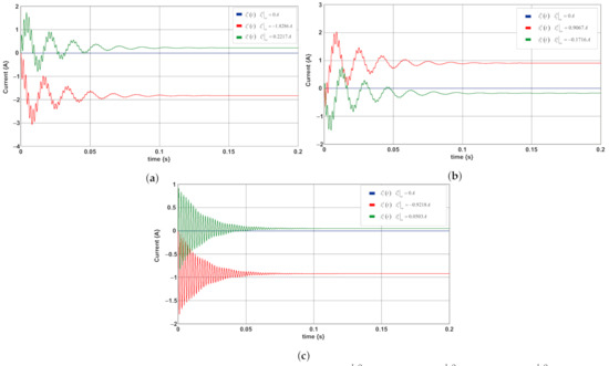
Figure 14. Dynamic and steady state responses on the (d, q, 0) axis: (a) $i_1^{dq0}\left(t\right)=\underline{f_3}\left(t\right)$; (b) $i_2^{dq0}\left(t\right)=\underline{f_4}\left(t\right)$; (c) $i_3^{dq0}\left(t\right)=\underline{f_{10}}\left(t\right)$.

The three phase currents $\left(a,b,c\right)$ for each branch are shown in Figure 15. These currents are obtained from the outputs $\underline{y}\left(t\right)={\left[\begin{array}{ccc}\underline{f_{21}}\left(t\right)& \underline{f_{25}}\left(t\right)& \underline{f_{23}}\left(t\right)\end{array}\right]}^T$ where $\underline{f_{21}}=i_1^{abc}$; $\underline{f_{25}}\left(t\right)=i_2^{abc}\left(t\right)$ and $\underline{f_{23}}\left(t\right)=i_3^{abc}\left(t\right)$.

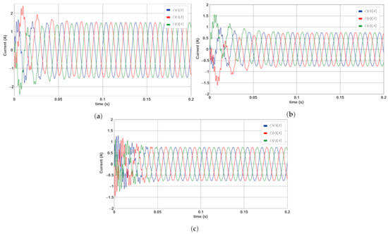
Figure 15. Three phase currents on the (a,b,c axis: (a) $\underline{f_{21}}\left(t\right)=i_1^{abc}\left(t\right)$; (b) $\underline{f_{25}}\left(t\right)=i_2^{abc}\left(t\right)$; (c) $\underline{f_{23}}\left(t\right)=i_3^{abc}\left(t\right)$.

Since this system is under balanced conditions, an equivalent reduced circuit per phase and with mesh currents can be solved [42,43]. In Appendix A, the check for mesh currents in the phasor approach of this case study is described.

However, the approach of this paper has the following characteristics: (1) we analyze under unbalanced conditions; (2) the mathematical model is not required; (3) the inverse of the state matrix is not necessary; (4) multibond graphs permit compaction; (5) systems have multi-domain energy; (6) the steady state response is symbolic.

5.2. Synchronous Generator

Synchronous generators represent one of the main sources of electrical energy in three-phase power systems. These synchronous generators are powered by hydroelectric or thermoelectric plants [42,43]. The schematic diagram of the cross-section of a synchronous generator with a pair of poles is illustrated in Figure 16. The field winding uses direct current and produces a magnetic field that induces voltages in the three phases in the armature windings.

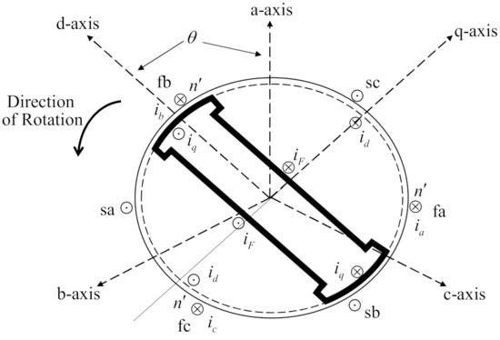
Figure 16. Schematic diagram of a three-phase synchronous machine.

The circuits used for the analysis of a synchronous generator are shown in Figure 17. The three-phase armature winding represents the stator circuits carrying current in all three phases, and the field winding describes the rotor circuit.

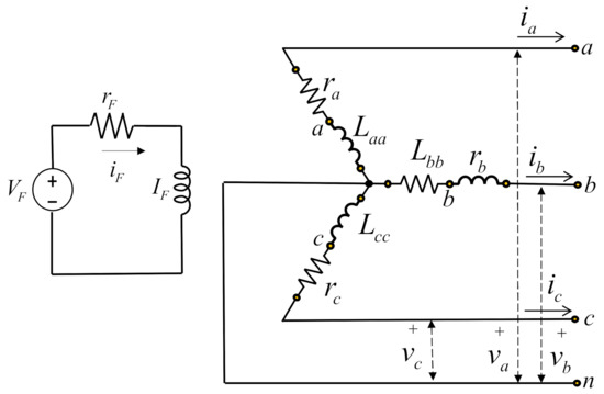
Figure 17. Stator and rotor circuits of a synchronous generator.

Figure 18 shows an MBGI of a synchronous generator on the d-q axis.

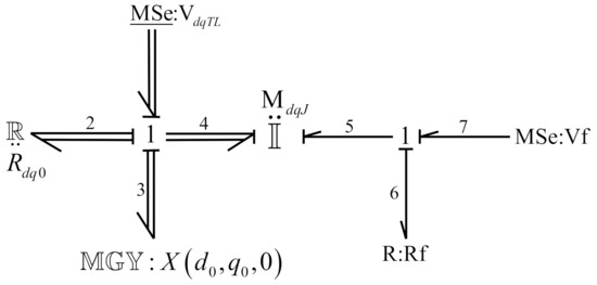
Figure 18. Multibond graph of a synchronous generator.

Figure 18 contains two sections:

• Stator circuits formed by three phase windings on the d-q axis where $R_d$ and $L_d$ denote the resistance and self-inductance on the d-axis circuit; $R_q$ and $L_q$ denote the resistance and self-inductance on the q-axis circuit; M is the mutual inductance between the stator and rotor; $V_d$ and $V_q$ are the supply voltages on $thed$-q axis; and the mechanical part whose elements are $T_L$ the mechanical torque, J the moment of inertia, and D the mechanical friction.
  This section is modeled by a multibond graph where $V_d$, $V_q$, and $T_L$ are effort sources that determine a multiport effort source $\underline{MSe}:V_{dqTL}$; the resistances on the d-q axis and the friction give a multiport resistance $\mathbb{R}:{\mathbf{R}}_{dqD}$; the inductances $L_d$, $L_q$, and J represent a multiport field $\mathbb{I}:M_{dqJF}$ with the mutual inductance M linking the inductance rotor circuit $L_f$; the relationships between the electrical circuits and the mechanical part are represented by a multiport gyrator $\mathbb{MGY}:X\left(d_o,q_0,0\right)$.
• The rotor circuit formed by the resistance and inductance on the field winding $R:R_f$ and $L_f$ and the supply voltage for this winding $MSe:V_f$.

In order to demonstrate that the multibond graph of Figure 18 represents a synchronous generator, the mathematical model in state variables is obtained.

The multibond graph has the following key vectors:

$$\begin{array}{ccc}\hfill \underline{x}\left(t\right)& =& \left[\begin{array}{c}\underline{p_4}\left(t\right)\\ p_5\left(t\right)\end{array}\right];\stackrel{•}{\underline{x}}\left(t\right)=\left[\begin{array}{c}\underline{e_4}\left(t\right)\\ e_5\left(t\right)\end{array}\right];\underline{z}\left(t\right)=\left[\begin{array}{c}\underline{f_4}\left(t\right)\\ f_5\left(t\right)\end{array}\right]\hfill \\ \hfill \underline{D_{in}}\left(t\right)& =& \left[\begin{array}{c}\underline{f_2}\left(t\right)\\ f_6\left(t\right)\end{array}\right];\underline{D_{out}}\left(t\right)=\left[\begin{array}{c}\underline{e_2}\left(t\right)\\ e_6\left(t\right)\end{array}\right];\underline{u}\left(t\right)=\left[\begin{array}{c}\underline{e_1}\left(t\right)\\ e_7\left(t\right)\end{array}\right]\hfill \\ \hfill \underline{I_{GY}}\left(t\right)& =& \underline{f_3}\left(t\right);\underline{O_{GY}}\left(t\right)=\underline{e_3}\left(t\right)\hfill \end{array}$$

The constitutive relations are:

$$\begin{array}{ccc}\hfill {\mathbf{F}}^{-1}& =& \left[\begin{array}{cc}{\mathbf{L}}_{dqJ}& {\mathbf{M}}_{sR}^T\\ {\mathbf{M}}_{sR}& L_f\end{array}\right]\hfill \end{array}$$

(77)

$$\begin{array}{ccc}\hfill \mathbf{L}& =& diag\left\{{\mathbf{R}}_{dqD},R_f\right\}\hfill \end{array}$$

(78)

$$\begin{array}{ccc}\hfill {\mathbf{X}}_{GY}& =& \mathbf{X}\left(-d_0,-q_0,0\right)=\left[\begin{array}{ccc}0& 0& P_{q0}\\ 0& 0& -P_{d0}\\ -P_{q0}& P_{d0}& 0\end{array}\right]\hfill \end{array}$$

(79)

where:

$$\begin{array}{ccc}\hfill {\mathbf{R}}_{dqD}& =& diag\left\{R_d,R_q,D\right\}\hfill \\ \hfill {\mathbf{L}}_{dqJ}& =& diag\left\{L_d,L_q,J\right\}\hfill \\ \hfill {\mathbf{M}}_{sR}& =& \left[\begin{array}{ccc}M& 0& 0\end{array}\right]\hfill \end{array}$$

and the multiport junction structure is defined by:

$$\left[\begin{array}{c}\underline{e_4}\left(t\right)\\ e_5\left(t\right)\\ \underline{f_3}\left(t\right)\\ \underline{f_2}\left(t\right)\\ f_6\left(t\right)\end{array}\right]=\left[\begin{array}{ccccccc}0& 0& -\mathbf{I}& -\mathbf{I}& 0& \mathbf{I}& 0\\ 0& 0& 0& 0& -1& 0& 1\\ 0& \mathbf{I}& 0& 0& 0& 0& 0\\ \mathbf{I}& 0& 0& 0& 0& 0& 0\\ 0& 1& 0& 0& 0& 0& 0\end{array}\right]\left[\begin{array}{c}\underline{f_4}\left(t\right)\\ f_5\left(t\right)\\ \underline{e_3}\left(t\right)\\ \underline{e_2}\left(t\right)\\ e_6\left(t\right)\\ \underline{e_1}\left(t\right)\\ e_7\left(t\right)\end{array}\right]$$

(80)

From (80):

$${\mathbf{S}}_{22}=0;{\mathbf{S}}_{11}^{22}=0;{\mathbf{S}}_{12}^{21}=0;{\mathbf{S}}_{21}^{12}=0$$

(81)

and substituting (81) into (15), (14), (12), and (13), the algebraic loop matrices are:

$$\begin{array}{ccc}\hfill {\mathbf{M}}_L& =& {\mathbf{Q}}_L=\mathbf{L}\hfill \end{array}$$

(82)

$$\begin{array}{ccc}\hfill {\mathbf{M}}_X& =& {\mathbf{Q}}_X={\mathbf{X}}_{GY}\hfill \end{array}$$

(83)

From (81)–(83), the state matrix (7) is reduced to:

$$\mathbf{A}=\left({\mathbf{S}}_{11}^{11}+{\mathbf{S}}_{11}^{12}{\mathbf{Q}}_X{\mathbf{S}}_{11}^{21}+{\mathbf{S}}_{12}^{11}{\mathbf{Q}}_L{\mathbf{S}}_{21}^{11}\right)\mathbf{F}$$

(84)

and the input matrix 8 is written as:

$$\mathbf{B}={\mathbf{S}}_{13}^{11}+{\mathbf{S}}_{11}^{12}{\mathbf{Q}}_X{\mathbf{S}}_{13}^{21}+{\mathbf{S}}_{12}^{11}{\mathbf{Q}}_L{\mathbf{S}}_{23}$$

(85)

From (77)–(80) and (82)–(85) the state space representation of the synchronous generator is given by:

$$\left[\begin{array}{c}\underline{e_4}\left(t\right)\\ e_5\left(t\right)\end{array}\right]=\left[\begin{array}{cc}-{\mathbf{R}}_{dqD}& 0\\ 0& -R_f\end{array}\right]\left[\begin{array}{c}\underline{f_4}\left(t\right)\\ f_5\left(t\right)\end{array}\right]+\left[\begin{array}{cc}\mathbf{X}\left(-d_0,-q_0,0\right)& 0\\ 0& 0\end{array}\right]\left[\begin{array}{c}\underline{f_4}\left(t\right)\\ f_5\left(t\right)\end{array}\right]+\left[\begin{array}{c}\underline{e_1}\left(t\right)\\ e_7\left(t\right)\end{array}\right]$$

(86)

To determine the steady state response, the MBGD of the synchronous generator is shown in Figure 19.

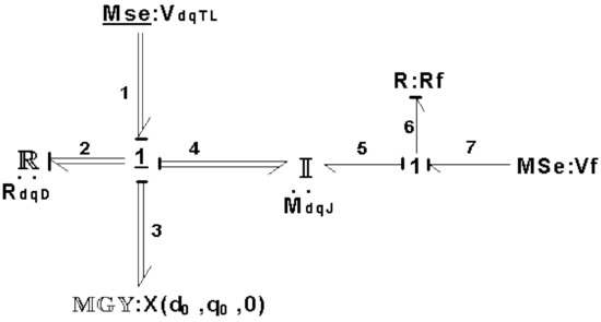
Figure 19. MBGD of a synchronous generator.

By assigning a derivative causality to the multiport storage elements defined by the bonds 4 and 7, then the bonds 2 and 6 have to change their causality in order to obtain the correct multibond graph. Hence, the new vectors for the multiport dissipation elements are given by:

$$\underline{D_{in}^d}\left(t\right)=\left[\begin{array}{c}\underline{e_2}\left(t\right)\\ e_6\left(t\right)\end{array}\right];\underline{D_{out}^d}\left(t\right)=\left[\begin{array}{c}\underline{f_2}\left(t\right)\\ f_6\left(t\right)\end{array}\right]$$

and its constitutive relation is:

$${\mathbf{L}}^d=diag\left\{{\mathbf{R}}_{dqD}^{-1},R_f^{-1}\right\}$$

(87)

and for the multiport gyrator is:

$${\mathbf{X}}_{GY}^d={\mathbf{X}}_{GY}$$

(88)

The multiport junction structure for the MBGD is defined by:

$$\left[\begin{array}{c}\underline{f_4}\left(t\right)\\ f_5\left(t\right)\\ \underline{f_2}\left(t\right)\\ f_6\left(t\right)\\ \underline{f_3}\left(t\right)\end{array}\right]=\left[\begin{array}{ccccccc}0& 0& 0& \mathbf{I}& 0& 0& 0\\ 0& 0& 0& 0& 1& 0& 0\\ 0& 0& 0& \mathbf{I}& 0& 0& 0\\ -\mathbf{I}& 0& -\mathbf{I}& 0& 0& \mathbf{I}& 0\\ 0& -1& 0& 0& 0& 0& 1\end{array}\right]\left[\begin{array}{c}\underline{f_4}\left(t\right)\\ f_5\left(t\right)\\ \underline{e_2}\left(t\right)\\ e_6\left(t\right)\\ \underline{e_3}\left(t\right)\\ \underline{e_1}\left(t\right)\\ e_7\left(t\right)\end{array}\right]$$

(89)

From (30) and (89), ${\mathbf{B}}^{\ast }$ is reduced to:

$${\mathbf{B}}^{\ast }={\mathbf{F}}^{-1}\left({\mathbf{J}}_{12}^{11}{\mathbf{P}}_L{\mathbf{J}}_{LB}\right)$$

(90)

From (2), (45) and (90), the steady state response is defined by:

$$\underline{z_{ss}}={\mathbf{J}}_{12}^{11}{\mathbf{P}}_L{\mathbf{J}}_{LB}\underline{u_{ss}}$$

(91)

also, ${\mathbf{J}}_{13}^{21}=0$ then ${\mathbf{J}}_{LB}$ is

$${\mathbf{J}}_{LB}={\mathbf{J}}_{23}$$

(92)

From (43), (87)–(89):

$${\mathbf{P}}_L=\left[\begin{array}{cc}{\mathbf{R}}_{dqD}^{-1}{\left(\mathbf{I}+{\mathbf{X}}_{GY}{\mathbf{R}}_{dqD}^{-1}\right)}^{-1}& 0\\ 0& R_f^{-1}\end{array}\right]$$

(93)

and substituting (89), (92) and (93) into (91), the steady state in a symbolic form is defined by:

$$\underline{z_{ss}}=\left[\begin{array}{cc}{\mathbf{R}}_{dqD}^{-1}{\left(\mathbf{I}+{\mathbf{X}}_{GY}{\mathbf{R}}_{dqD}^{-1}\right)}^{-1}& 0\\ 0& R_f^{-1}\end{array}\right]\underline{u_{ss}}$$

(94)

By using physical variables:

$$\underline{z_{ss}}=\left[\begin{array}{c}{\left(\underline{f_4}\right)}_{ss}\\ {\left(f_5\right)}_{ss}\end{array}\right]=\left[\begin{array}{c}{\left(f_4^d\right)}_{ss}\\ {\left(f_4^q\right)}_{ss}\\ {\left(f_4^J\right)}_{ss}\\ {\left(f_5\right)}_{ss}\end{array}\right]=\left[\begin{array}{c}{\left(i_d\right)}_{ss}\\ {\left(i_q\right)}_{ss}\\ {\left(w\right)}_{ss}\\ {\left(i_f\right)}_{ss}\end{array}\right]$$

and system inputs:

$$\underline{u_{ss}}=\left[\begin{array}{c}{\left(\underline{e_1}\right)}_{ss}\\ {\left(e_7\right)}_{ss}\end{array}\right]=\left[\begin{array}{c}{\left(e_1^d\right)}_{ss}\\ {\left(e_1^q\right)}_{ss}\\ {\left(e_1^{T_L}\right)}_{ss}\\ {\left(e_7\right)}_{ss}\end{array}\right]=\left[\begin{array}{c}{\left(V_d\right)}_{ss}\\ {\left(V_q\right)}_{ss}\\ {\left(T_L\right)}_{ss}\\ {\left(V_f\right)}_{ss}\end{array}\right]$$

and (79), (87) and (94), the steady state for each state variable is described by:

$$\left[\begin{array}{c}{\left(f_4^d\right)}_{ss}\\ {\left(f_4^q\right)}_{ss}\\ {\left(f_4^J\right)}_{ss}\\ {\left(f_5\right)}_{ss}\end{array}\right]=\left[\begin{array}{cccc}{P}_{d0}^2+D{R}_q& P_{d0}{P}_{q0}& -P_{q0}{R}_q& 0\\ P_{d0}{P}_{q0}& P_{q0}^2+D{R}_d& P_{d0}{R}_d& 0\\ P_{q0}{R}_q& -P_{d0}{R}_d& R_d{R}_q& 0\\ 0& 0& 0& {\displaystyle \frac{\Delta }{R_f}}\end{array}\right]\frac{1}{\Delta }\left[\begin{array}{c}{\left(e_1^d\right)}_{ss}\\ {\left(e_1^q\right)}_{ss}\\ {\left(e_1^{T_L}\right)}_{ss}\\ {\left(e_7\right)}_{ss}\end{array}\right]$$

(95)

where:

$$\Delta =D{R}_d{R}_q+P_{d0}^2{R}_d+P_{q0}^2{R}_q$$

Considering balanced conditions applied to the synchronous generator:

$$v^{abc}\left(t\right)=\left[\begin{array}{c}100cos\left(377t\right)\\ 100cos\left(377t-120\right)\\ 100cos\left(377t+120\right)\end{array}\right]\mathrm{V}$$

and using Park’s transformation:

$$\left[\begin{array}{c}{\left(e_1^d\right)}_{ss}\\ {\left(e_1^q\right)}_{ss}\\ {\left(e_1^{T_L}\right)}_{ss}\\ {\left(e_7\right)}_{ss}\end{array}\right]=\left[\begin{array}{c}122.4744\mathrm{V}\\ 3.1903\times {10}^{-10}\mathrm{V}\\ 100\mathrm{N}·\mathrm{m}\\ 30\mathrm{V}\end{array}\right]$$

the numerical parameters of the elements for the d-axis are $R_d=0.1\mathrm{\Omega }$ and $L_d=1.7\mathrm{H}$, for the q-axis are $R_q=1\mathrm{\Omega }$ and $L_q=1.64\mathrm{H}$, the mutual inductance between d and q axes is $M=1.55\mathrm{H}$, for the field circuit are $R_f=1\mathrm{\Omega }$, $L_f=1.65\mathrm{H}$, and the mechanical part is given by $J=2.37N-m-s^2$ and $D=1$. The initial flux linkages are: $P_{d0}=0.002\mathrm{A}·\mathrm{H}$ and $P_{q0}=0.1279\mathrm{A}·\mathrm{H}$. By substituting all the numerical values of the parameters into (95), the steady state of the co-energy vector of the synchronous generator is given by:

$$\left[\begin{array}{c}{\left(f_4^d\right)}_{ss}\\ {\left(f_4^q\right)}_{ss}\\ {\left(f_4^J\right)}_{ss}\\ {\left(f_5\right)}_{ss}\end{array}\right]=\left[\begin{array}{c}-46.642\mathrm{A}\\ 1.988\mathrm{A}\\ 994.03\mathrm{rad}/\mathrm{s}\\ 30.00\mathrm{A}\end{array}\right]$$

(96)

In order to prove the obtained results, the simulation of the synchronous generator using the 20-SIM software is shown in Figure 20.

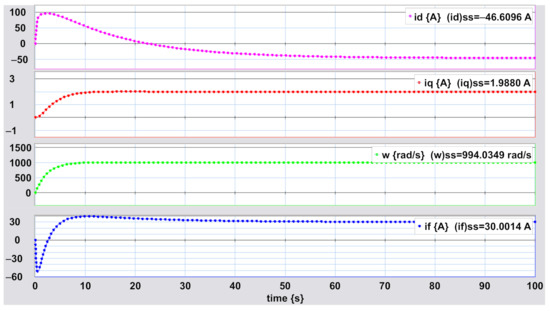
Figure 20. Physical variables’ performance for the synchronous generator: $i_d$, $i_q$, w, and $i_f$.

The dynamic behavior based on the MBGI of Figure 18 for the synchronous generator is obtained and shown in Figure 20. The steady state for the variables $i_d$, $i_q$, w, and $i_f$ is illustrated, and the results given in (96) are verified.

Finally, Figure 21 shows the three-phase electrical current $\left(i_a,i_b,i_c\right)$ produced by the synchronous generator. Under balanced conditions, the currents $\left(i_d,i_q\right)$ are transformed to $\left(i_a,i_b,i_c\right)$ by using Park’s inverse transformation. Note that when the dynamic period is over, the steady state response is reached.

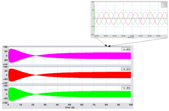
Figure 21. Three-phase electrical current: $i_a$, $i_b$, and $i_c$.

Finally, the analysis and methodologies developed for bond graphs using the junction structure can be extended with this paper for multibond graphs.

6. Conclusions

The steady state response of LTI systems represented by multibond graph models is presented. The multiport junction structure of a multibond graph in an integral causality assignment (MBGI) that determines the state space of an LTI system is proposed. This MBGI admits multiport storage elements in integral and derivative causality assignments that represent linearly independent and dependent state variables, respectively. By assigning a derivative causality to all storage elements, a multibond graph in a derivative causality assignment (MBGD) is obtained. The relationships between MBGI and MBGD give the direct determination of the steady state of a multiport system.

Two case studies are modeled by multibond graphs: a three-phase electrical system and a synchronous generator. In both cases, the steady state using this approach is obtained. Finally, in order to verify the steady state behavior of the state variables, the simulation results are shown. The advantages for applying multibond graphs with respect to bond graphs for multibody systems are clear: the short notation, junction structure, and mathematical model are compact. Furthermore, the proposed junction structure to determine the characteristics (structural observability, structural controllability, stability, control design) in the physical domain can be key for new results.

References

- Nise, N.S. Control Systems Engineering; Wiley: New York, NY, USA, 2000. [Google Scholar]
- Pagnozzi, M.; Coletta, G.; Leone, G.; Catani, V.; Esposito, L.; Fiorillo, F. A Steady State Model to Simulate Groundwater Flow in Unconfined Aquifer. Appl. Sci. 2020, 10, 2708. [Google Scholar] [CrossRef]
- Chang, C.-W.; Liu, C.-H.; Wang, C.-C. A Modified Polynomial Expansion Algorithm for Solving The Staedy-State Allen-Cahn Equation for Heat Transfer in Thin Films. Appl. Sci. 2018, 8, 983. [Google Scholar] [CrossRef]
- Senturia, S.D. Microsystem Design; Kluwer Academic Publishers: Dordrecht, The Netherlands, 2002. [Google Scholar]
- Yu, M.; Lu, H.; Wang, H.; Xiao, C.; Lan, D. Compound Fault Diganosis and Sequential Prognosis for Electric Scooter with Uncertainties. Actuators 2020, 9, 128. [Google Scholar] [CrossRef]
- Barjuei, E.S.; Caldwell, D.G.; Ortiz, J. Bond Graph Modeling and Kalman Filter Observer Design for an Industrial Back-Support Exoskeleton. Designs 2020, 4, 53. [Google Scholar] [CrossRef]
- Zrafi, R.; Ghedira, S.; Besbes, K. A Bond Graph Approach for the Modeling and Simulation of a Buck Converter. J. Low Power Electron. Appl. 2018, 8, 2. [Google Scholar] [CrossRef]
- Lin, C.; Shen, Z.; Yu, J.; Li, P.; Huo, D. Modeling and Analysis of Characteristics of a Piezoelectric-Actuated Micro-/Nano Compliant Platform Using Bond Graph Approach. Micromachines 2018, 9, 498. [Google Scholar] [CrossRef]
- Algar, A.; Codina, E.; Freire, J. Bond Graph Simulation of Error Propagation in Position Estimation of a Hydraulic Cylinder Using Los Cost Accelerometers. Energies 2018, 11, 2603. [Google Scholar] [CrossRef]
- Van der Weff, K. Kinematic and Dynamic Analysis of Mechanisms, a Finite Element Approach; Delft University Press: Delft, The Netherlands, 1977. [Google Scholar]
- Zhang, W.J.; van der Werff, K. Automatic communication from a neutral object model of mechanism to mechanism analysis programs based in a finite element approach in a software enviroment for CADCAM of mechanisms. Finite Elem. Anal. Des. 1998, 28, 209–239. [Google Scholar] [CrossRef]
- Moon, W.-K.; Busch-Vishniac, I.J. A finite-element equivalent bond graph modeling approach with application to the piezoelectric thickness vibrator. J. Acoust. Am. 1993, 93, 3496. [Google Scholar] [CrossRef]
- Pal, S.K.; Talamantes-Silva, J.; Linkens, D.A.; Howard, I.C. Bond graph and finite element analyses of temperature distribution in a hot rolling process: A comparative study. Proc. Inst. Mech. Eng. Part I J. Syst. Control 2007, 221, 653–661. [Google Scholar] [CrossRef]
- Nakhaeinejad, M.; Lee, S.; Bryant, M.D. Finite element bond graph model of rotors. In Proceedings of the 2010 Spring Simulation Multiconference, Orlando, FL, USA, 11–15 April 2010; pp. 1–6. [Google Scholar]
- Breedveld, P.C. A bond graph algorithm to determine the equilibrium state of a system. J. Franklin Inst. 1984, 318, 71–75. [Google Scholar] [CrossRef]
- Gawthrop, P.J. Bicausal bond graphs. In Proceedings of the International Conference on Bond graph modeling (ICBGM’95), Las Vegas, NV, USA, 15–18 January 1995; pp. 83–88. [Google Scholar]
- Ngwompo, R.F.; Scarvada, R.; Thomasset, D. Inversion of linear time-invariant SISO systems modeled by bond graph. J. Frankl. Inst. 1996, 333, 157–174. [Google Scholar] [CrossRef]
- Bideaux, E.; Marquis-Favre, W.; Scavarda, S. Equilibrium set investigation using bicausality. Math. Comput. Model Dynam Syst. 2006, 12, 127–140. [Google Scholar] [CrossRef]
- Gonzalez, G.; Galindo, R. Steady state determination using bond graphs for systems with singular state matrix. Proc. IMechE Part I J. Syst. Control Eng. 2011, 225, 887–901. [Google Scholar] [CrossRef]
- Gawthrop, P. Computing Biomolecular System Steady-States. IEEE Trans. Nanobiosci. 2018, 17, 36–43. [Google Scholar] [CrossRef]
- Breedveld, P.C. Multibond Graph Elements in Physical Systems Theory. J. Frankl. Inst. 1985, 319, 1–36. [Google Scholar] [CrossRef]
- Borutzky, W.; Dauphin-Tanguy, G.; Thoma, J.U. Advances in bond graph modeling: Theory, software, applications. Math. Comput. Simul. 1995, 39, 465–475. [Google Scholar] [CrossRef]
- Boruttzky, W. Bond Graphs for Modeling, Control and Fault Diagnosis of Engineering Systems, 2nd ed.; Springer: Berlin/Heidelberg, Germany, 2017. [Google Scholar]
- Behzadipour, S.; Khajepour, A. Causality in vector bond graphs and its application to modeling of multi-body dynamic. Syst. Simul. Model. Pract. Theory 2006, 14, 279–295. [Google Scholar] [CrossRef]
- Breedveld, P.C. Stability of rigid body rotation from a bond graph perspective. Simul. Model. Pract. Theory 2009, 17, 92–106. [Google Scholar] [CrossRef]
- Breedveld, P.C. Essential gyrators and equivalence rules for 3-port junction structures. J. Franklin Inst. 1984, 318, 77–89. [Google Scholar] [CrossRef]
- Breedveld, P.C. Decomposition of multiport elements in a revised multibond graph notation. J. Franklin Inst. 1984, 318, 253–273. [Google Scholar] [CrossRef]
- Golo, G.; der Schaft, A.V.; Breedveld, P.C.; Marschke, B.M. Hamiltonian formulation of bond graphs. In Nonlinear and Hybrid Systems in Automotive Control; University of Gronigen, Johann Bernoulli, Institute for Mathematics and Computer Science: Groningen, The Netherlands, 2003; Volume 19, pp. 351–372. [Google Scholar]
- Nu nez, I.; Breedveld, P.C.; Weustink, P.B.T.; Gonzalez, G. Steady-state power flow analysis of electrical power systems modeled by 2- dimensional multibond graphs. In Proceedings of the International Conference on Integrated Modeling and Analysis in Applied Control and Automation, Bergeggi, Italy, 21–23 September 2015; pp. 39–47. [Google Scholar]
- Avalos, G.G.; Ayala, G.; Gallegos, N.B.; Padilla, A. Linearization of a class of non-linear systems modeled by multibond graphs. Math. Comput. Model. Dyn. 2019, 25, 284–332. [Google Scholar] [CrossRef]
- Abbes, M.; Farhat, A.; Mami, A.; Dauphin-Tanguy, G. Pseudo bond graph model of coupled heat and mass transfers in a plastic tunnel greenhouse. Simul. Model. Pract. Theory 2010, 18, 1327–1341. [Google Scholar] [CrossRef]
- Boudon, B.; Malburet, F.; Carmona, J. Simulation of a helicopter’s main gearbox semi-active suspension with bond graphs. Multibody Syst. Dyn. 2016, 39, 60–64. [Google Scholar]
- Sarker, M.; Rideout, D.G.; Butt, S.D. Dynamic model for 3D motions of a horizontal oil well BHA with wellbore stick-slip whirl interaction. J. Pet. Sci. Eng. 2017, 157, 482–506. [Google Scholar] [CrossRef]
- Pfeifer, M.; Caspart, S.; Hampel, S.; Muller, C.; Krebs, S.; Hohmann, S. Explicit port-Hamiltonian formulation of multi-bond graphs for an automated model generation. Automatica 2020, 120, 109121. [Google Scholar] [CrossRef]
- Lee, J.-N.; Nikravesh, P.E. Steady-state analysis of multibody systems with reference to vehicle dynamics. Nonlinear Dyn. 1994, 5, 181–192. [Google Scholar]
- Hendy, H.; Rui, X.; Zhou, Q. Controller Parameters tuning based on Transfer matrix method for multibody systems. Adv. Mech. Eng. 2015. [Google Scholar] [CrossRef]
- Dauphin-Tanguy, G.; Rahmani, A.; Sueur, C. Bond graph aided design of controlled systems. Simul. Pract. Theory 1999, 7, 493–513. [Google Scholar] [CrossRef]
- Sueur, C.; Dauphin-Tamguy, G. Bond-graph Approach for Structural Analysis of MIMO Linear Systems. J. Franklin Inst. 1991, 328, 55–70. [Google Scholar] [CrossRef]
- Avalos, G.G.; Gallegos, N.B. Quasi-steady state model determination for systems with singular perturbations modeled by bond graphs. Math. Comput. Model. Dyn. 2013, 19, 483–503. [Google Scholar] [CrossRef]
- Karnopp, D.C.; Margolis, D.L.; Rosenberg, R.C. System Dynamics Modeling and Simulation of Mechatronic Systems; Wiley, John & Sons: Hoboken, NJ, USA, 2000. [Google Scholar]
- Banerjee, S. Dynamics for Engineers; Wiley: Hoboken, NJ, USA, 2005. [Google Scholar]
- Kundur, J.R. Power System Stability and Control; Mc. Graw-Hill: New York, NY, USA, 1994. [Google Scholar]
- Anderson, P.M. Power System Control and Stability; The Iowa State University Press: Ames, IA, USA, 1977. [Google Scholar]
- Zhou, K.; Doyle, J.C. Essentials of Robust Control; Prentice-Hall: Upper Saddle River, NJ, USA, 1998. [Google Scholar]
Publisher’s Note: MDPI stays neutral with regard to jurisdictional claims in published maps and institutional affiliations. |
© 2021 by the authors. Licensee MDPI, Basel, Switzerland. This article is an open access article distributed under the terms and conditions of the Creative Commons Attribution (CC BY) license (http://creativecommons.org/licenses/by/4.0/).