The Extreme Function Theory for Damage Detection: An Application to Civil and Aerospace Structures

Featured Application

This paper presents an application of Extreme Function Theory (EFT) and Gaussian Processes (GPs) to perform mode shape-based damage detection and Structural Health Monitoring (SHM).

Abstract

Any damaged condition is a rare occurrence for mechanical systems, as it is very unlikely to be observed. Thus, it represents an extreme deviation from the median of its probability distribution. It is, therefore, necessary to apply proper statistical solutions, i.e., Rare Event Modelling (REM). The classic tool for this aim is the Extreme Value Theory (EVT), which deals with uni- or multivariate scalar values. The Extreme Function Theory (EFT), on the other hand, is defined by enlarging the fundamental EVT concepts to whole functions. When combined with Gaussian Process Regression (GPR), the EFT is perfectly suited for mode shape-based outlier detection. In fact, it is possible to investigate the structure’s normal modes as a whole rather than focusing on their constituent data points, with quantifiable advantages. This provides a useful tool for Structural Health Monitoring, especially to reduce false alarms. This recently proposed methodology is here tested and validated both numerically and experimentally for different examples coming from Civil and Aerospace Engineering applications. One-dimensional beamlike elements with several boundary conditions are considered, as well as a two-dimensional plate-like spar and a frame structure.

1. Introduction

The identification and localisation of damage in one-, two-, or three-dimensional structures through their mode shapes are widespread in the Structural Health Monitoring (SHM) community. It is well known that by inserting a localised discontinuity, the mode shapes diverge from their usual deflection path [1]. This principle has been extensively applied to investigate damage-induced variations in the mode shapes slope or curvature for both 1-dimensional beam-like [2] and 2-dimensional plate-like [3,4] structures. In this regard, a review of classic approaches can be found in Reference [5]. These approaches consider modal curvatures [6], mode shape rotations [7], and/or several other Damage-Sensitive Features (DSFs) based on the structure’s eigenvectors. In particular, mode shapes-based methods are preferred over other modal parameters for damage localisation, since they inherently have the spatial resolution needed for this specific task [8,9]. However, even having established that the mode shapes and derived quantities can be exploited as a reliable and spatially dense DSFs, it remains to define how these features can be used for anomaly detection.

The changes in the mode shapes can be detected, e.g., through a Machine Learning (ML) process, trained exclusively on the mode shapes extracted from the current state of the structure. This can be applied both to a known pristine condition or to an already-damaged structure, since the basis of outlier detection is to identify variations from the configuration “as it is” [10]. Indeed, no method can actually detect “damage”, but rather its effects on the structural properties [11]. That is to say, the damage detection algorithms are inherently subject to false positives as they could mislabel noisy data for actual deviations. This problem is very commonly encountered with measurements from real-life applications.

The economic, social, and safety concerns of structural false alarms must not be neglected, as they are one of the major reasons which still hampers the perceived usefulness of SHM and continuous monitoring, limiting their spreading. For example, for any fixed- or rotary-wing aircraft, an onboard Health and Usage Monitoring System (HUMS) would be useless, if not even dangerous, if constantly sending false alarms. These are all major practical issues; the latter one, for instance, can be arguably considered the main factor behind the industry reluctance to apply SHM systems at large scale in the last two decades [12], and the reduction of false alarms is still a matter of research as of 2020 [13].

The main concept of this work departs from the consideration that structural damages are rare events. Therefore, assuming a normal distribution for damage occurrences is both statistically unprincipled and potentially inaccurate with all the resulting risks. Thus, Rare Event Modelling (REM) should be preferably applied. For scalar values, this can be done following the well-known Extreme Value Theory (EVT), also known as Extreme Value Statistics (EVS) [14]. As the name suggests, the EV framework—a part of the more general theory of the order statistics—deals with the statistics of extremes. This represents an ideal framework for data-driven thresholding [13], not only for damage assessment but generally for several applications of novelty detection (as reviewed in Reference [15]). The EVT framework for novelty detection has been firstly proposed by Roberts [16], especially for applications with biomedical signals [17]. For SHM purposes, the EVT was firstly introduced by Sohn et al. [18] and applied on time series. Park et al. [19] further deepened these studies considering ARX models in the frequency domain. Sohn and colleagues subsequently used the EVS framework for the analysis of delaminated composite panels, with the use of wavelets [20] and time-reversal acoustics [21]. Sundaram et al. [22] used multivariate EV Statistics and Gaussian Mixture Models on 8 performance and 4 vibrational parameters extracted from data collected from aerospace gas-turbine engines.

However, the basic concepts of EVT can be easily extended to whole functions to define the so-called Extreme Function Theory (EFT, [23]). The rationale is that the same statistical tools applied commonly on scalar values can be applied on 1- or multi-dimensional functions (like the mode shapes), not differently from what, e.g., is done for Gaussian Processes (GPs) in comparison to Gaussian distributions. This was, for instance, utilised by Papatheou et al. [24] to perform damage detection in offshore wind turbines based on their recorded power curves.

Another important aspect is that, according to the Fisher–Tippett–Gnedenko theorem [25,26], any extreme distribution on the lower or upper tail converges to only three possible extreme distributions—the Gumbel, Fréchet, and Weibull distribution families, also known as type I, II and III EV distributions—which can be unified in the Generalised Extreme Value (GEV) formulation. This happens independently from the parent distribution; that is to say, the proposed approach is not limited by the assumption of a Gaussian distribution, which—while being commonly used in structural mechanics and dynamics on the basis of the well-known Central Limit Theorem (CLT) [27]—could be not always consistent with the experimental data (e.g., in case of skewed distributions).

In this work, GP Regression and EFT are combined to define a “normality” data-driven model, fitted over the mode shapes collected from the structure “as it is”, and then to check for damage-related deviations from this model [28]. The use of a statistical framework purposely crafted on rare events greatly reduced the number of false positives. The rest of this paper is organised as follows: The theoretical framework of the procedure is described in Section 2. The results of the investigations performed on the numerically simulated case studies are reported in Section 3. The experimental validation is described in Section 4. Section 5 (Conclusions) ends this paper.

2. Gaussian Processes and Extreme Function Theory

In the specific case of interest, the problem can be stated as follows. Let $i=1,\dots ,n$ be the index of $n$ examples taken from a population of functional data. Each $i$-th example is an identified mode shape ${\mathit{\phi }}_{\mathit{i}}$, i.e., a vector of $j=1,\dots ,n_i$ modal coordinates ${\phi }_{i,j}$ observed at a finite number of corresponding spatial coordinates ${\mathrm{x}}_{i,j}$. From a theoretical standpoint, there is no requirement that the $n$ mode shapes have the same number of coordinates nor the same location. This is the first strong point of EFT in comparison to EVT, as the functions can be collected from different sensor arrangements—even if, for practical concerns, it is more reliable to consider a fixed number and position of the output channels. Importantly, ${\mathrm{x}}_{i,j}$ can be a scalar for a 1-dimensional beam element, or a pair ${\mathrm{x}}_{i,j}=\left\{{\xi }_{i,j},{\eta }_{i,j}\right\}$ for a 2-dimensional plate-like structure (and so on). For simplicity’s sake, all the rest of this discussion will focus on the 1-dimensional case but the formulation for higher dimensionalities can be straightly derived.

There are two subsequent aims. The first one is to build the “normality” model $ℳ$ from the pairs of training data $\left\{x_{\mathit{i}},{\mathit{\phi }}_{\mathit{i}}\right\}$, collected from a given structure excited in the current conditions (assumed as a baseline for outlier detection). Once the model is defined, the second step is to discern if a test set $\left\{x_{\mathit{i}}^{\ast },{\mathit{\phi }}_{\mathit{i}}^{\ast }\right\}$ (in this case, $i=1,\dots ,n^{\ast }$) belongs or not to the tails of the distribution $ℳ$. The first part can be achieved with the classic GP Regression, which is here briefly recalled for completeness, while the EFT comes in the second part.

2.1. The Gaussian Process (GP) Regression

Being the mode shapes $\mathit{\phi }$ a function of the space variable $\mathit{x}$, it is possible to define a GP prior over this latent variable, in the general form

$$f\left(\mathit{x}\right)~GP\left(m\left(\mathit{x}\right),k\left(\mathit{x},{\mathit{x}}^{\prime }\right)\right),$$

(1)

not dissimilarly from how a normal distribution is uniquely defined by its mean and variance, the GP of the general process $\mathrm{f}\left(\mathit{x}\right)$ can be defined uniquely by its mean function

$$m\left(\mathit{x}\right)=E\left[f\left(\mathit{x}\right)\right]$$

(2)

and on the covariance matrix

$$k\left(\mathit{x},{\mathit{x}}^{\prime }\right)=E\left[\right(f\left(\mathit{x}\right)-m\left(\mathit{x}\right)\left)\right(f\left({\mathit{x}}^{\prime }\right)-m\left({\mathit{x}}^{\prime }\right)\left)\right]$$

(3)

where $\mathrm{E}\left[·\right]$ denotes the expectation. Throughout this whole discussion, a zero-mean and squared-exponential (SE) covariance function will be applied (the exact formulation will be discussed later; other less frequent options exist and a discussion on the topic can be found in Reference [29]).

If $\mathit{f}=\mathrm{f}\left(\mathit{x}\right)$ indicates the set of the function values at the training points $\mathit{X}$ (note that the training vectors have been assembled into a matrix form) and ${\mathit{f}}^{\ast }$ a set of test outputs at a new set of points ${\mathit{X}}^{\ast }$, according to the zero-mean prior it is possible to define

$$\left[\begin{array}{c}\mathit{f}\\ {\mathit{f}}^{\ast }\end{array}\right]~\mathcal{N}\left(0,\left[\begin{array}{cc}K\left(\mathit{X},\mathit{X}\right)& K\left(\mathit{X},{\mathit{X}}^{\ast }\right)\\ K\left({\mathit{X}}^{\ast },\mathit{X}\right)& K\left({\mathit{X}}^{\ast },{\mathit{X}}^{\ast }\right)\end{array}\right]\right),$$

(4)

where $\mathrm{K}\left(X^{\ast },X\right)\in {ℝ}^{n^{\ast }\times n}$ is a matrix with the terms defined by the covariances evaluated at all pairs of test and training points (the same applies for $\mathrm{K}\left(X,X\right)$, $\mathrm{K}\left(X,X^{\ast }\right)$, and $\mathrm{K}\left(X^{\ast },X^{\ast }\right)$).

The posterior distribution is defined by conditioning the joint prior on the observations, resulting (for an ideally noise-free scenario) in

$$\begin{array}{cc}p({\mathit{f}}^{\ast }|{\mathit{X}}^{\ast },\mathit{X},\mathit{f})~& \mathcal{N}(K\left({\mathit{X}}^{\ast },\mathit{X}\right)K{\left(\mathit{X},\mathit{X}\right)}^{-1}\mathit{f},K\left({\mathit{X}}^{\ast },{\mathit{X}}^{\ast }\right)\\ & -K\left({\mathit{X}}^{\ast },\mathit{X}\right)K{\left(\mathit{X},\mathit{X}\right)}^{-1}K\left(\mathit{X},{\mathit{X}}^{\ast }\right)).\end{array}$$

(5)

By considering the measurement noise as i.i.d. Gaussian noise $ϵ$ with variance ${\mathsf{\sigma }}_{\mathrm{n}}^2$, one can define

$$\mathit{\phi }=f\left(\mathit{x}\right)+ϵ$$

(6)

thus, Equation (5) becomes

$$p({\mathit{f}}^{\ast }|{\mathit{X}}^{\ast },\mathit{X},\mathit{\phi })~\mathcal{N}\left(m\left({\mathit{f}}^{\ast }\right),cov\left({\mathit{f}}^{\ast }\right)\right)$$

(7)

with the predictive mean

$$m\left({\mathit{f}}^{\ast }\right)=K\left({\mathit{X}}^{\ast },\mathit{X}\right){[K\left(\mathit{X},\mathit{X}\right)+{\sigma }_n^2\mathit{I}]}^{-1}\mathit{\phi }$$

(8)

and the predictive covariance matrix

$$cov\left({\mathit{f}}^{\ast }\right)=K\left({\mathit{X}}^{\ast },{\mathit{X}}^{\ast }\right)-K\left({\mathit{X}}^{\ast },\mathit{X}\right)\left[K\left(\mathit{X},\mathit{X}\right)+{\sigma }_n^2\mathit{I}{]}^{-1}K\left(\mathit{X},{\mathit{X}}^{\ast }\right)\right).$$

(9)

At this point, it is evident that the only step remaining before obtaining the normality model is to define its covariance and the added noise. It was already assumed that this latter depends solely on ${\sigma }_n^2$. In the simpler (i.e., 1-dimensional) case, the aforementioned SE covariance function can be formulated as

$$k_{\phi }\left(x_p,x_q\right)={\sigma }_f^2\exp \left[-\frac{1}{2l}{\left(x_p-x_q\right)}^2\right]+{\sigma }_n^2{\delta }_{p,q}$$

(10)

where $k_{\phi }$ is the covariance of the noisy target set $\mathit{\phi }$, ${\sigma }_f^2$ is the variance of the function, $l$ is the length-scale parameter, ${\delta }_{p,q}$ is the Kronecker delta, and $x_p,x_q$ are the locations of the training data sets corresponding to the respective indices. ${\sigma }_f^2$, $l$, and ${\sigma }_n^2$ are the free parameters who need to be set from the data and are collectively known as the GP Regression hyperparameters $\theta$. Their setting requires an optimisation, which is generally performed by maximising the log marginal likelihood with respect to the hyperparameters. However, in general, the minimisation, rather than the maximisation, is performed; therefore, it is more practically convenient (without any theoretical drawback) to define directly the negative log marginal likelihood (NLML) as

$$logp(\mathit{\phi }|X,\theta =l,{\sigma }_f,{\sigma }_n)=\frac{1}{2}{\mathit{\phi }}^T{K}_{\phi }^{-1}\mathit{\phi }+\frac{1}{2}log\left|K_{\phi }\right|-\frac{n}{2}log2\pi$$

(11)

where $K_{\phi }$ indicates the covariance matrix of the noisy test set. The iterative minimisation is performed through a Conjugated Gradient Optimisation (CGO) algorithm; the process stops when the difference in NLML values are smaller than a set tolerance. At that point, the hyperparameters can be considered as the best fitting for the SE covariance function on the training data considered. The GP Regression over the training data can be therefore easily achieved and the metamodel $ℳ$ defined.

2.2. The Extreme Function Theory and the Complete Procedure

Consider the posterior distribution as defined in Equation (7), set accordingly to the hyperparameters optimised as described in the previous Section. By definition, a GP distribution over functions is a multivariate normal (Gaussian) distribution, thus the probability distribution $z=p(f^{\ast }|{\mathit{X}}^{\ast },\mathit{X},\mathit{\phi })$ will follow the form

$$z=\frac{1}{\sqrt[2]{2{\pi }^D\left|K^{\ast }\right|}}\exp \left[-\frac{1}{2}{\left({\mathit{f}}^{\ast }-m^{\ast }\right)}^T{K}^{\ast }{}^{-1}\left({\mathit{f}}^{\ast }-m^{\ast }\right)\right]$$

(12)

where $m^{\ast }=m\left(f^{\ast }\right)$, $K^{\ast }=cov\left(f^{\ast }\right)$, and $D$ is the dimensionality of $x^{\ast }$ (here onwards it is assumed that a single mode shape is tested at a time; even if it is theoretically possible to test jointly a set of more mode shapes at once, this will have little practical sense). Therefore, the whole test set $\left\{x_i^{\ast },{\mathit{\phi }}_i^{\ast }\right\}$ is reduced to a single scalar value corresponding to its likelihood. In turn, this can be used to fit an EV distribution over its left tail (i.e., for a very low probability of occurrence, as expected for damaged conditions). The lower 10% of the validation dataset was used to this aim. Specifically, the Cumulative Distribution Function (CDF) is here fitted on low values of the Gaussian log probability $\ln \left(z\right)$. For the GEV minima distribution, the exact formulation of the CDF is

$$L\left(\ln \left(z\right),\lambda ,\delta ,\gamma \right)=1-\exp \left(-{\left(1+\gamma \left(\frac{\lambda -\ln \left(z\right)}{\delta }\right)\right)}^{\frac{1}{\gamma }}\right)$$

(13)

where $\lambda ,\delta ,$ and $\gamma$ represent, in the same order, the location, scale, and shape parameter of the GEV distribution, which needs to be inferred from the data. Importantly, the shape parameter $\gamma$ controls the specific form of the limit minima distribution, which simplifies in a Gumbel distribution for $\gamma \to 0$, in a Weibull distribution if $\gamma <0$, or in a Fréchet distribution if $\gamma >0$ [30].

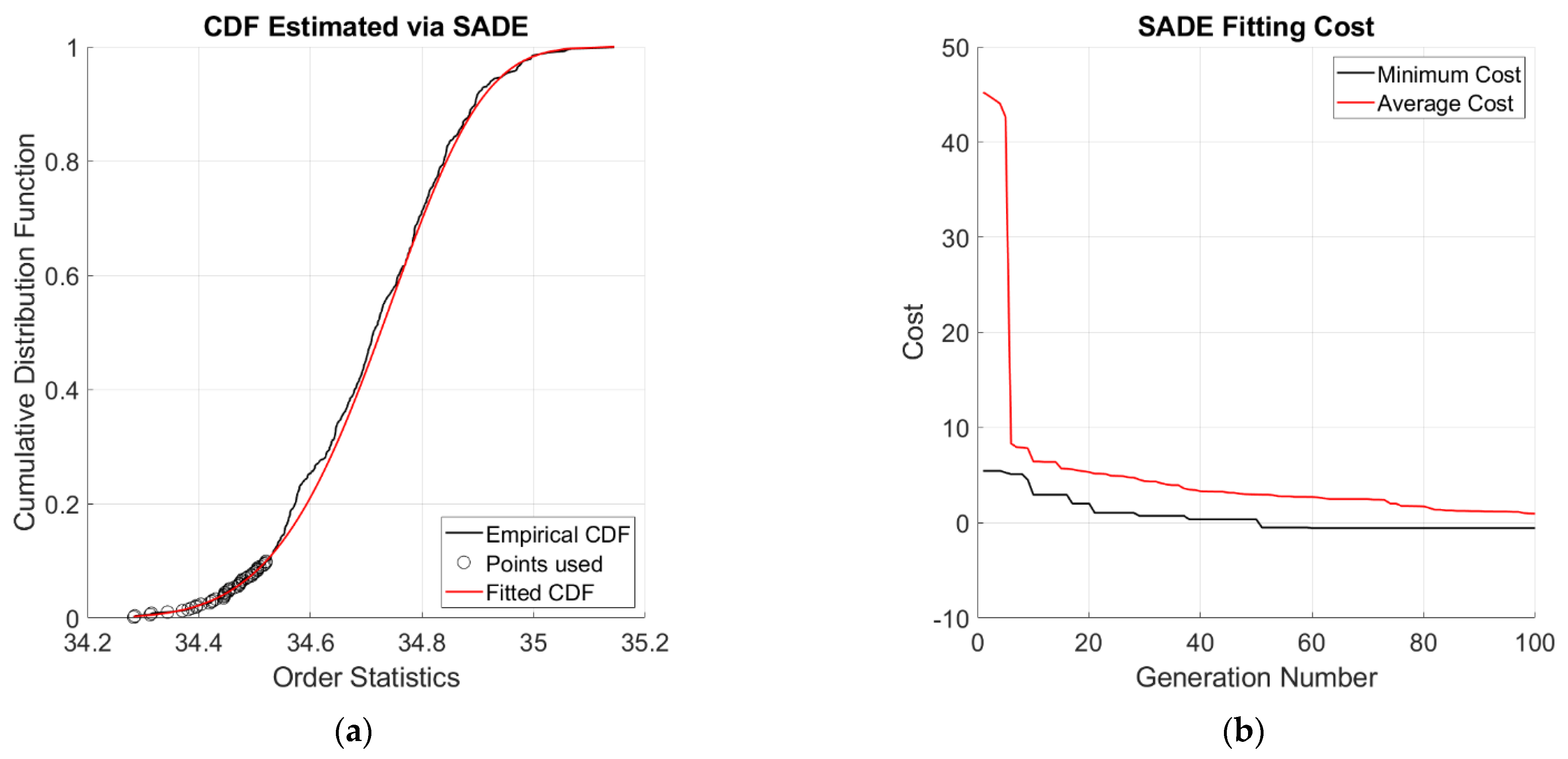
The estimation of the GEV parameters has been achieved utilising a Differential Evolution (DE) algorithm, as suggested in Reference [31]; specifically, the Self-Adaptive Differential Evolution (described in Reference [32]) was applied, considering 10 runs, 100 generations, and population size equal to 30. The Normalised Mean Square Error (NMSE) was set as the target cost function, minimised against the empirical CDF calculated according to the Hazen plotting position; an example is depicted in Figure 1. Having constructed the CDF it is then possible to define a threshold value $\ln z_{\lim }$ in correspondence of an arbitrarily chosen quantile $\alpha$. Here in this study, $\alpha =$ 1% was imposed. This completes the description of the whole procedure.

2.3. Test of the Performances of the Procedure

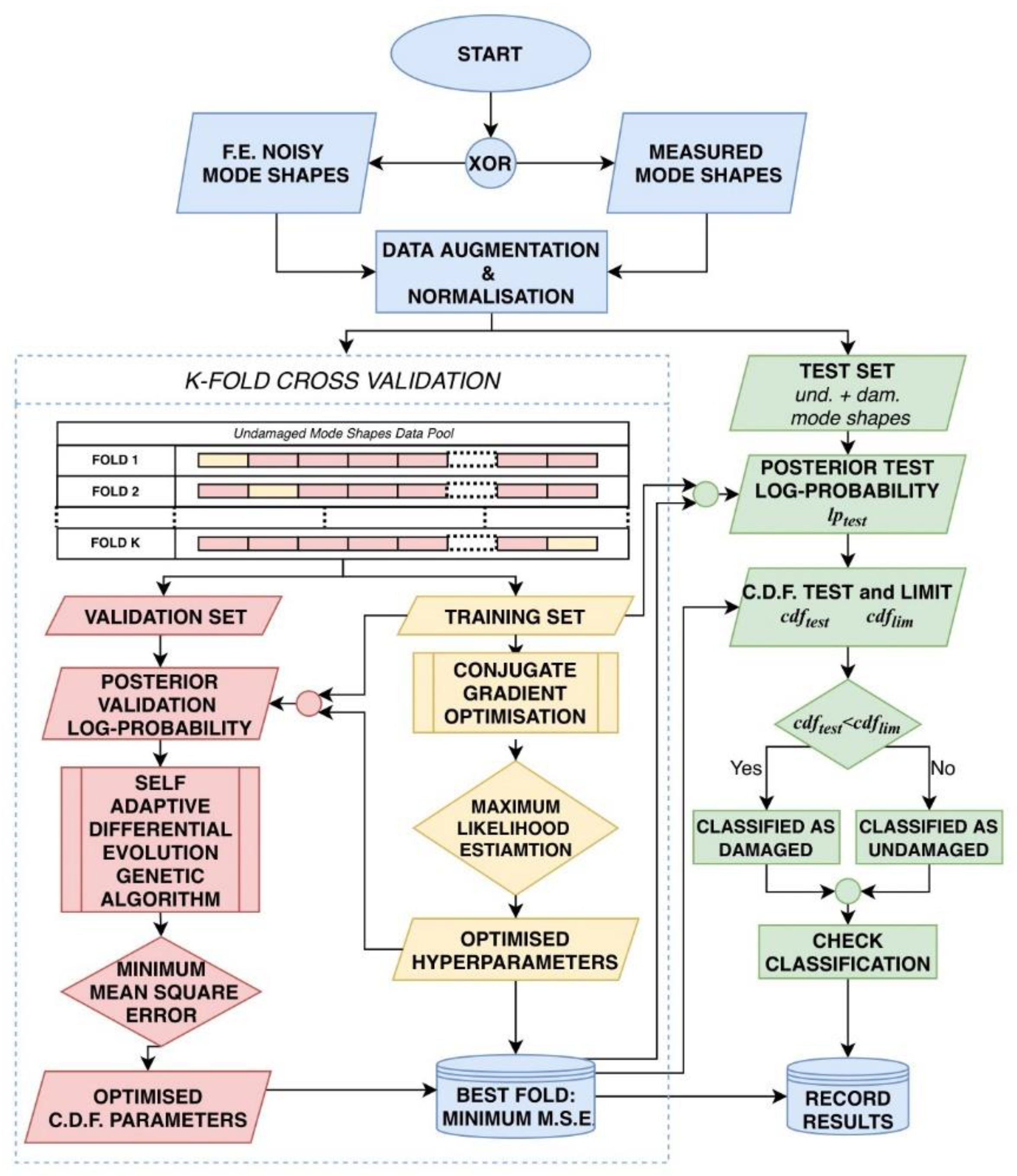
To quantitatively estimate the performances of the described approach, this was tested on numerically simulated and experimental datasets with known damage conditions. For this purpose, three datasets—training, validation, and test—are defined. The training and the validation datasets, needed to preliminary set and validate the normality model offline, are made up of functions drawn from the undamaged conditions, while the test set includes both damaged and undamaged states. For clarity’s sake, the several steps described in the previous Subsection are graphically depicted in Figure 2.

In comparison to a preliminary version of the algorithm described in Reference [28] and tested for simple cantilever beams, the following enhancements have been included.

Firstly, a data augmentation strategy was applied to overcome the limited amount of available measured data (numerical data were generated with the same scarcity as for the real data from the experimental case study). Dealing with the feature of transverse displacements, the latent function $\mathit{f}\left(\mathit{x}\right)$ of Equation (6) is the resulting mean of all the original mode shapes and the resulting standard deviation indicates how data are spread out from the average. Both the mean and the standard deviation were evaluated for each channel, to consider the distribution for the specific measurement point and not of the whole dataset. After generating the desired number of noise-free copies, white Gaussian noise was added by iteratively reducing the Signal-to-Noise-Ratio (SNR) until the artificially simulated data fell completely within the set limits. In this case, the range was arbitrarily chosen to be ±2σ and not to cover the whole ±3σ range, since this restriction strengthens the “normality” condition (i.e., undamaged conditions, not far from the median value). It should be noted that data coming from the augmentation process are involved in the training and validation steps, while only original data are tested to assess the efficiency of the algorithm.

As a second improvement, a step of k-fold cross-validation was added, to avoid overfitting of model parameters estimations. In contrast to the usual validation procedure, the k-th holdout fold subset was used to train the Gaussian Process and estimate its hyperparameters, while keeping the remaining $k-1$ folds for the CDF estimation and model testing. This inversion in the common paradigm of using the larger part of data for training step is due to the need to take into consideration only the lower 10% of the available data to estimate the minima form of CDF as defined in Equation (13). Subsequently, the training (TR), validation (VA), and test (TS) subsets were assembled from the given d structural configurations considered as the “normality” model (generally $d=1$, the integer measurements data set) and $d^{\ast }$ structural configurations considered as damaged, each with $n$ actual observations and $n^{\ast }$ artificial copies.

Table 1. The procedure settings of the damage detection.

Number of Observations (n)	50 for the Experimental Case Study 100 for the Numerical Case Studies
Data Augmentation (n*)	500
Range Augmentation	$\pm 2\sigma$
K-Fold (k)	5
Training Set (TR)	$\frac{1}{k}\left(\frac{n}{2}+n^{\ast }\right)$
Validation Set (VA)	$\left(1-\frac{1}{k}\right)\left(\frac{n}{2}+n^{\ast }\right)$
Test Set (TS)	$\frac{n}{4}$

describes the procedure settings, as applied for all the numerical and the experimental case studies for consistency.

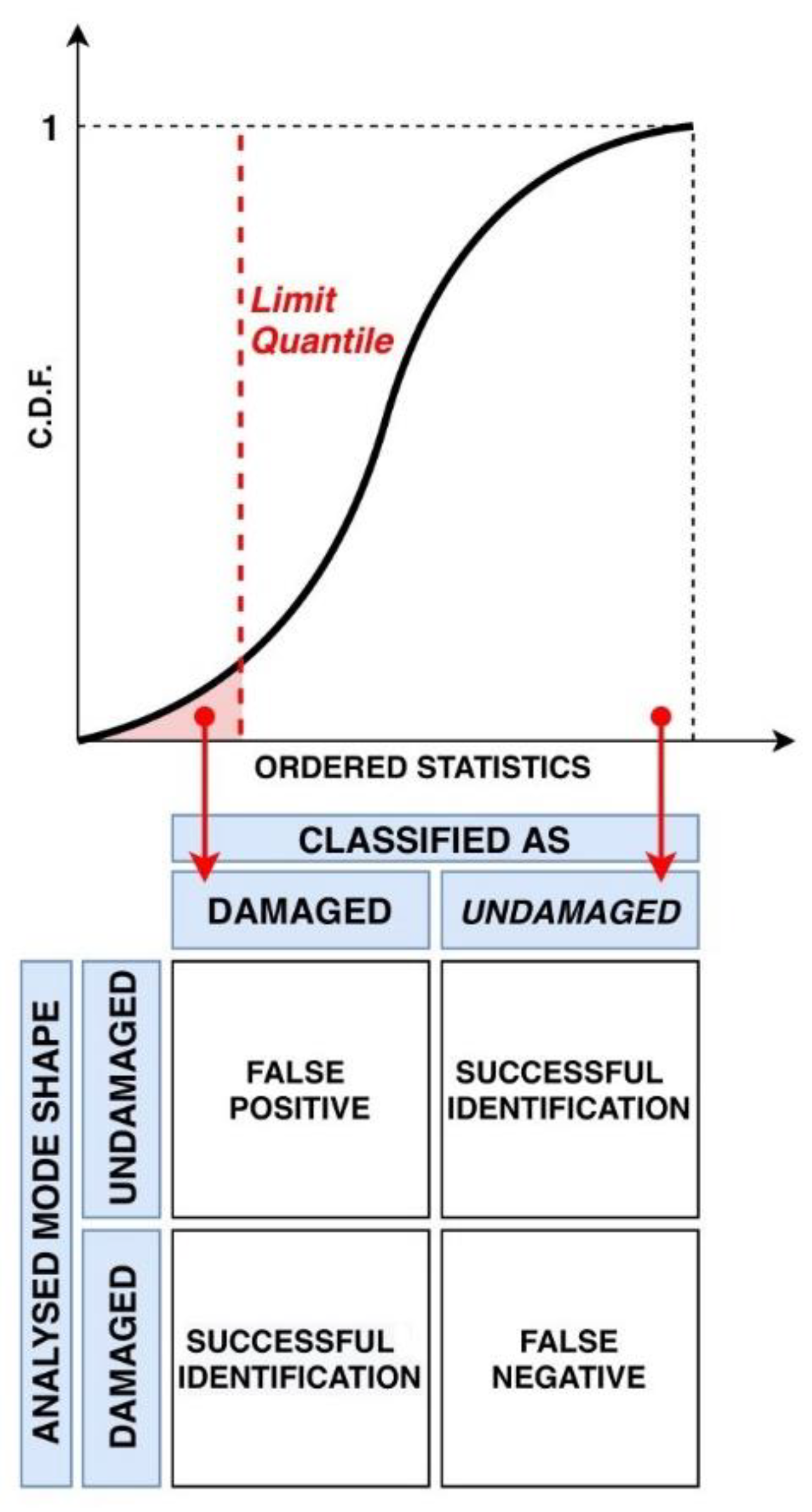
As said, the test set contains both undamaged (${\mathit{\phi }}_{und}$) and damaged (${\mathit{\phi }}_{dam}$) mode shapes. When a ${\mathit{\phi }}_{und}$ is classified as damaged, it is recorded as a false positive; on the other hand, misclassified ${\mathit{\phi }}_{dam}$ are considered as false negatives. Otherwise, as pictorially described in Figure 3, the results are labelled as true positives and true negatives.

3. Numerical Simulations

The procedure is firstly validated on a numerically-simulated beam with different boundary conditions. Then, for more complex structures, the proposed approach is firstly validated on two other numerical datasets.

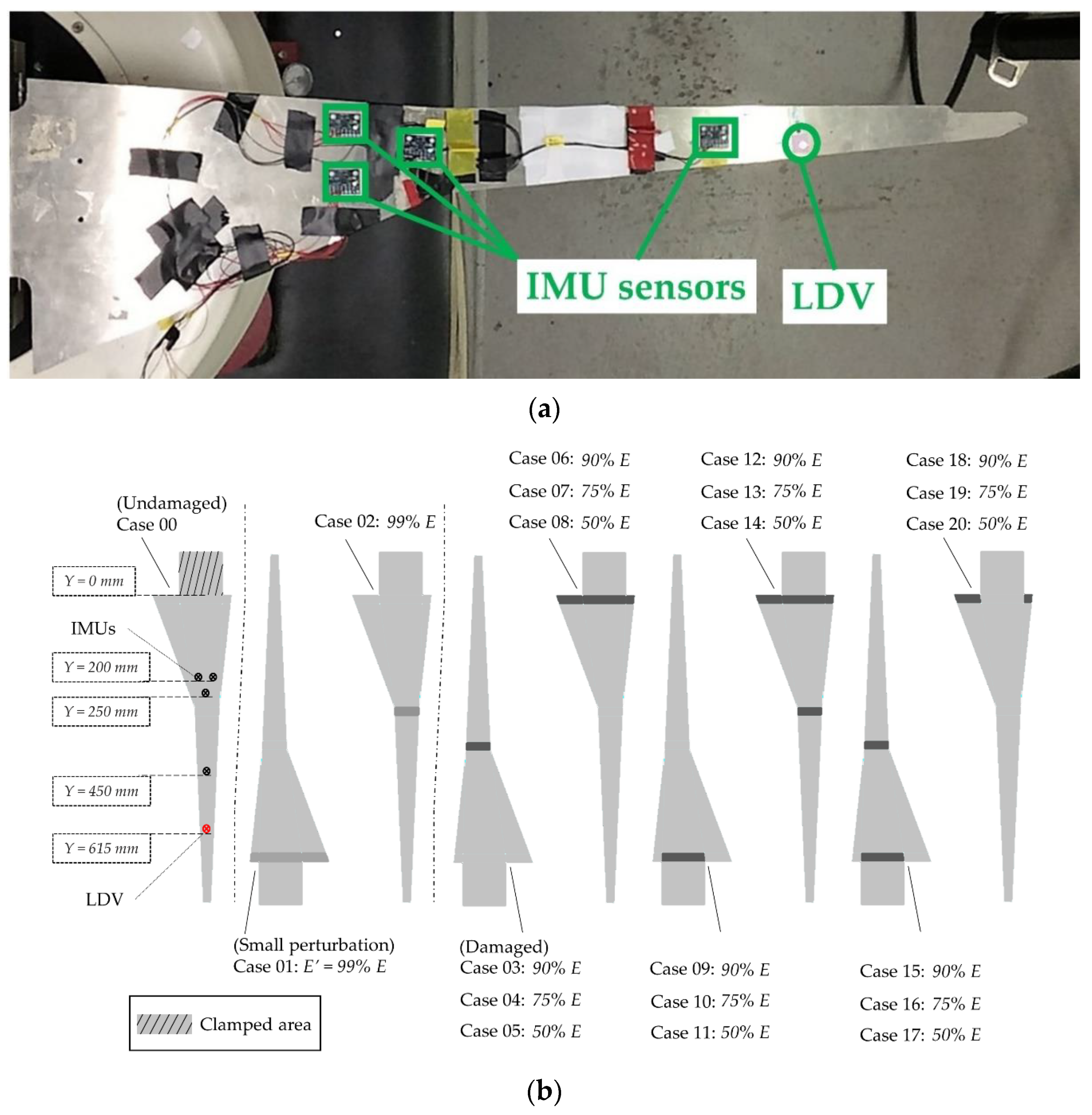
The first case study comes from an aerospace application and involves the High Aspect Ratio (HAR) aluminium spar of the XB-1 wing prototype [33]. The spar—portrayed in Figure 4a—can be seen as a thin, plate-like structural element with a peculiar shape. Due to its large flexibility, the spar may undergo large flap-wise oscillations [34,35] and it is therefore highly subject to the insurgence of fatigue damage, especially close to its clamped end and in its mid-length at the section where the width taper angle change. The simple Finite Elements (FE) model utilised here was realised in Ansys^® Mechanical APDL; 400 8-noded, 6-degrees-of-freedom-per-node quadratic shell elements were utilised. The main mechanical and geometrical properties are reported in

Table 2. Mechanical and geometrical properties of the spar.

Density ρ	2893	kg/m3
Young’s modulus E	5.90 × 1010	Pa
Poisson’s ratio v	0.26	-
Damping ratio	0.8634	%
Free length (clamp to tip) ltip	706	mm
Thickness t	2	mm
Max width at clamped section bmax	180.00	mm
Width at the taper angle change (l = 258 mm) b258	56.10	mm
Min width at the tip section bmin	17.04	mm

(the values of the parameters derive from preovius studies described in [36]). The model parameters were updated with vibrational data coming from laser Doppler vibrometer (LDV) and video acquisitions [36], extracted by means of the Fast Relaxed Vector Fitting (FRVF) approach [37,38]. Five output channels (located at the positions of the 4 Inertial Measurement Units and of the LDV target used during the experimental acquisitions, as represented in Figure 4a) were utilised to define the mode shapes. Several levels of reduced Young’s modulus were applied to the portions highlighted in Figure 4b to simulate 20 scenarios [10]. In particular, the first two states (01 and 02) are intended to represent small perturbations from the undamaged baseline, where the variations are not sufficiently marked to be defined certainly as actual damage. This simulates the possible statistical variability of the identified mechanical properties; therefore, these states should preferably be labelled as false positives by a reliable (i.e., not hypersensitive) damage detection procedure. Indeed, it was found that, when trained on noiseless mode shapes only, the procedure does not discern these small perturbations from the normal (undamaged) model.

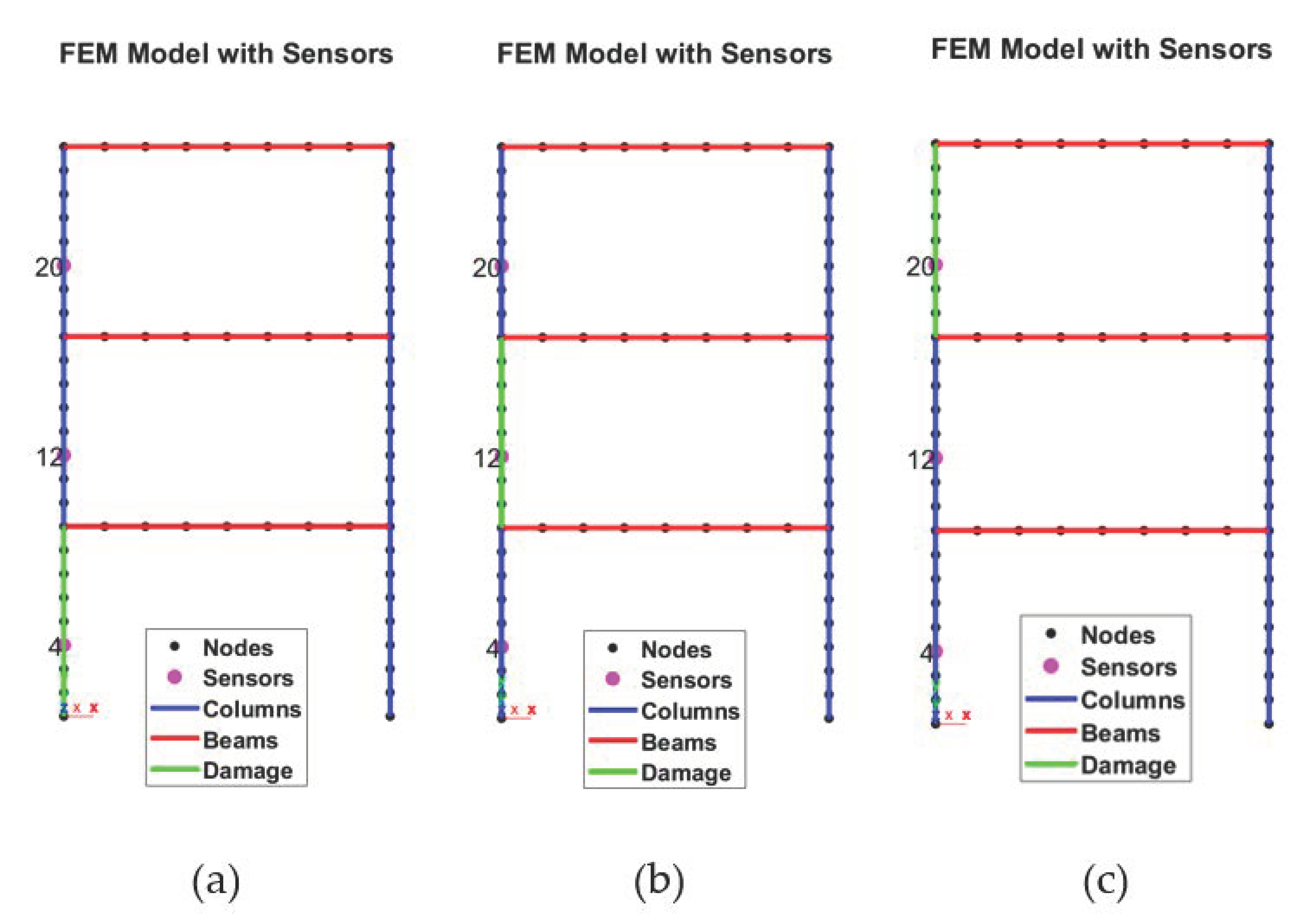
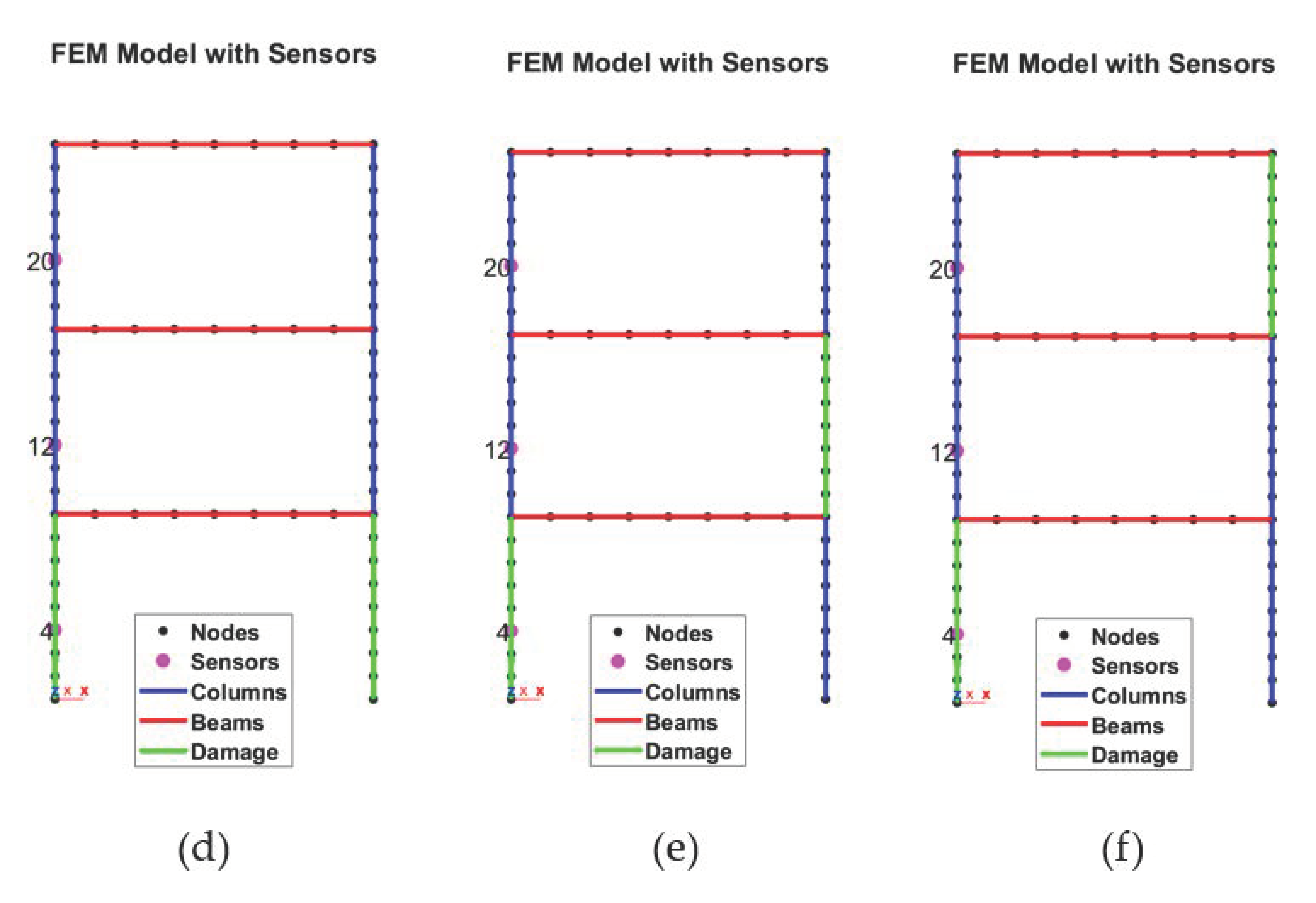
The second numerical case study comes from a civil engineering application and is intended to model a simple multi-storey frame structure, which will serve as the experimental benchmark in the next Section. The FE (Figure 5) model, developed utilising the StaBil 2.0 MatLab Toolbox [39], was set as follows. 8 beam elements per column and per beam were used, totalling 72. The Timoshenko model was applied for all elements.

To mimic the experimental setup which will be described in the next section, the Young’s modulus of the beams $E_{beam}$ was set as two orders of magnitude larger than its counterpart for the columns ($E_{column}$). This allows to approximate the structural system as a shear-type frame structure; therefore, a single channel per floor is enough to capture its main vibrational modes. Three output channels were considered as virtual sensors, located at nodes #4, #12, and #20 (indicated by the purple dots in Figure 5). The main technical details are reported in

Table 3. Details of the frame FE model.

Density ρ	2700	kg/m3
Young’s modulus (columns) $E_{column}$	6.90 × 1010	Pa
Young’s modulus (beams) $E_{beam}$	6.90 × 1012	Pa
Poisson’s ratio v	0.3	-
Column length (per storey)	177	mm
Beam length	305	mm
Width of the column/beam cross-section	6	mm
Height of the column/beam cross-section	25	mm

. The column tracts highlighted in green are the ones where the damage was inserted (as a stiffness reduction equal to 25% or 50%).

3.1. Results for the Beam (1-Dimensional) FE Model

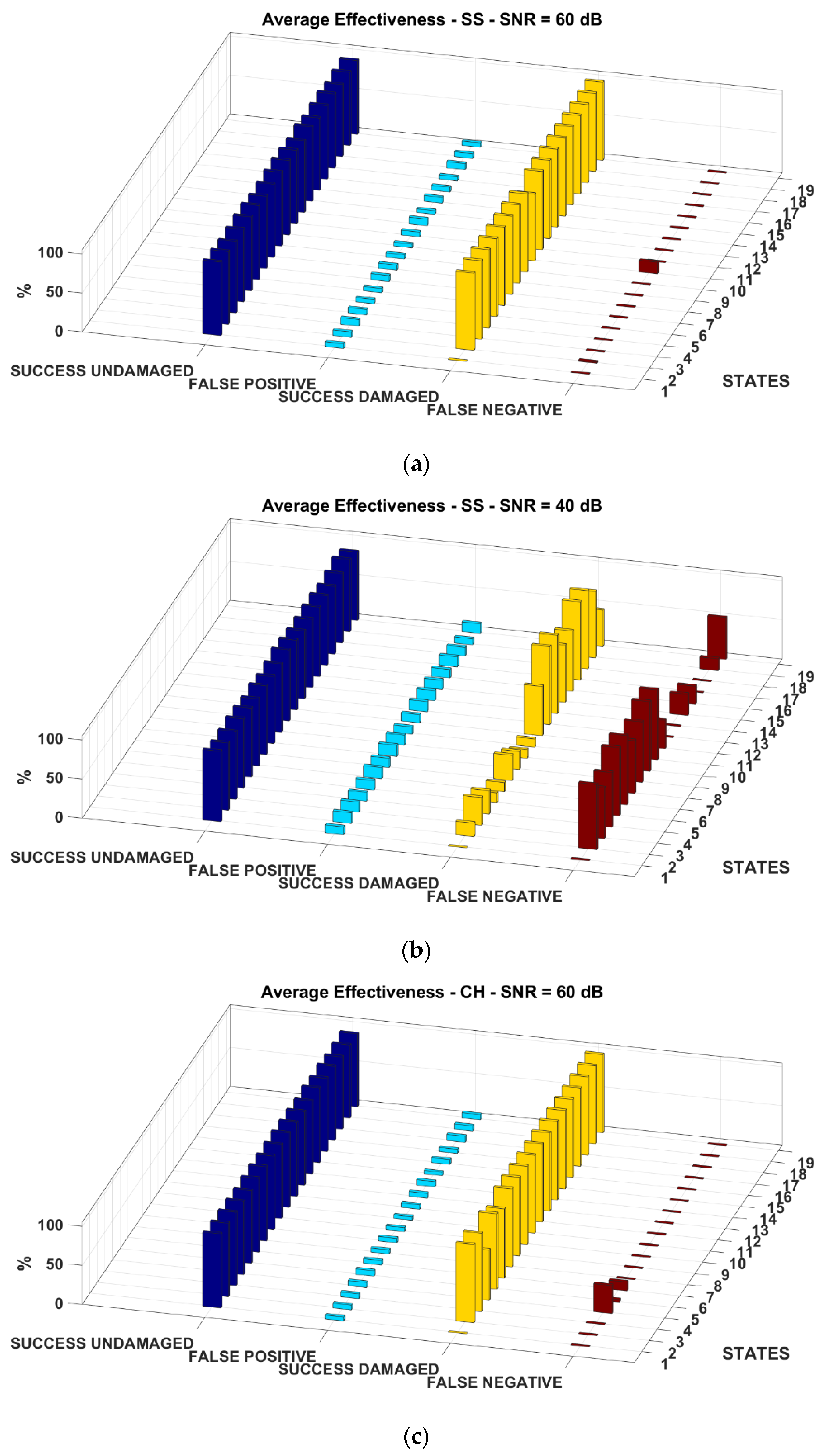
Figure 6 shows the results for two examples, the symmetrical pinned-pinned structural configuration and the asymmetrical clamped-pinned configuration. The method can be nevertheless applied to any statically determined or undetermined scenario. As it will be shown in the next Section, the same is valid for frame structures as well as 2-dimensional or more complex structures. Two levels of artificially added noise have been considered—SNR = 60 dB and 40 dB, respectively. The first state depicted in Figure 6 corresponds to the undamaged structure. Consider that in this state, no damage was to be detected, so the successful damage identifications and false alarms are both zeroed. The remaining states are defined for nine crack locations, equally spaced of 10% l between 0 and l, and for a crack depth equal to 10% of the thickness (states 2 to 10) or 20% (states 11 to 19). It can be noticed how these states, being affected by larger damage, are more easily detected by the algorithm as foreseeable. Only the first mode shape is reported for conciseness, calculated at the nodes #10, #30, and #49 (numbered sequentially, left to right, with the beam discretised in 50 elements).

It can be appreciated that the rate of success strictly depends on the position of the damage. This issue is well-known for any mode shape-based approach. In general, this depends on the position of the mode shapes nodes and antinodes and can be solved by considering, e.g., different mode shapes at once [40].

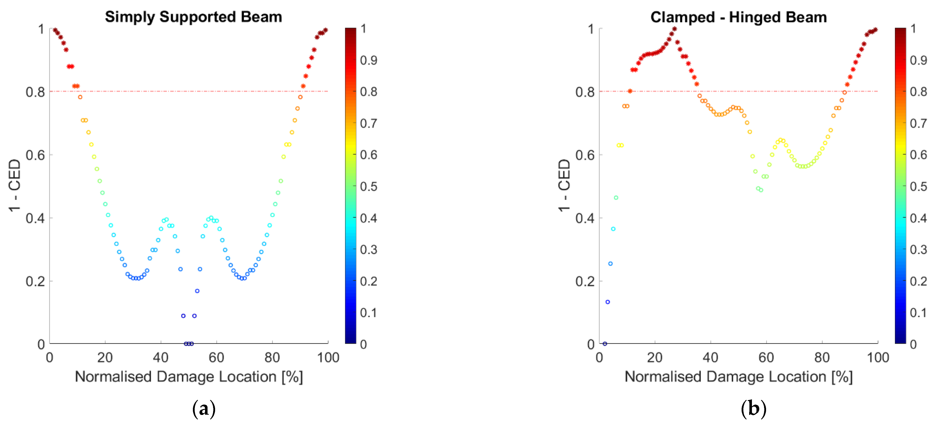
For a baseline-based approach as the one proposed here, the normalisation to a unit maximum displacement also causes some regions of the damaged mode shape to be very close to the ones of the undamaged scenario, reducing the detectability of the damage. This arises from the eigenproblem being underdetermined and therefore the eigenvectors being defined only up to scale.

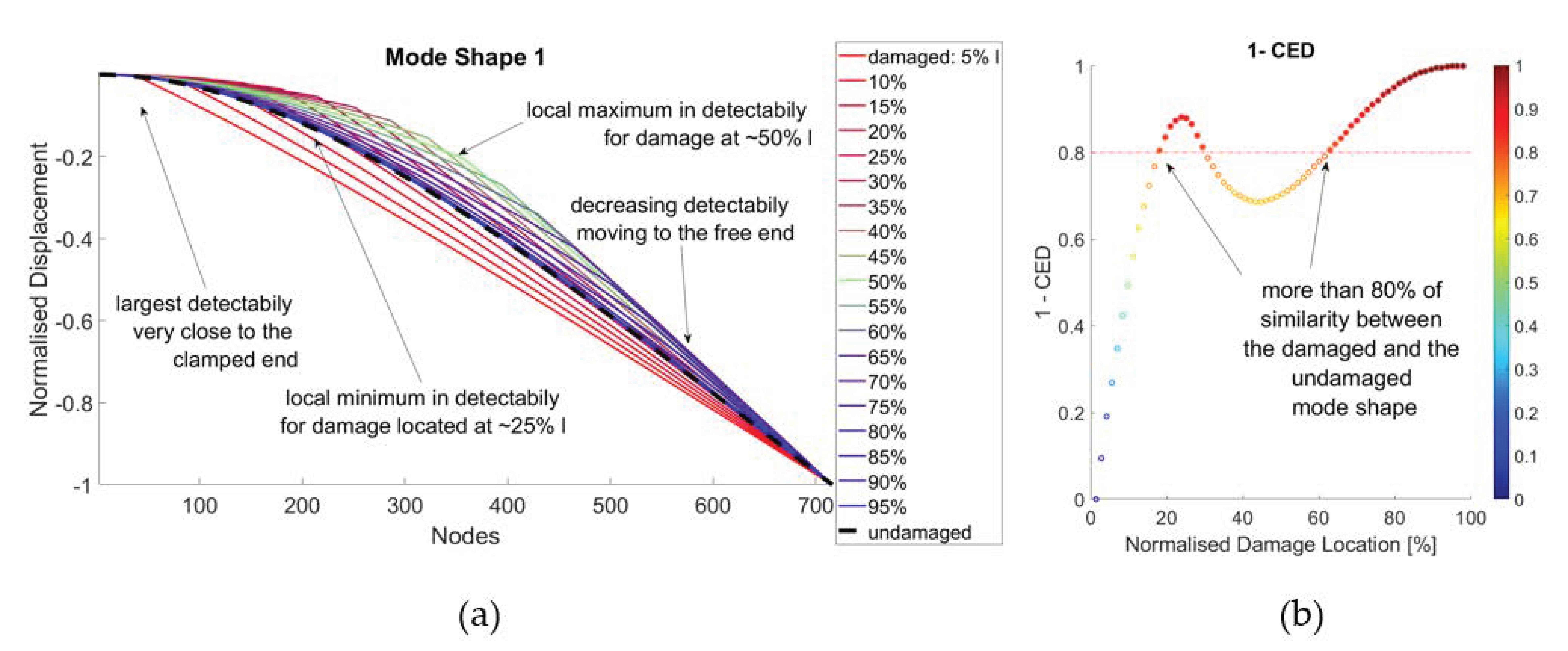
This difference between the normalised damaged and baseline mode shapes is here considered in terms of cumulative Euclidean distance (CED) and it is exemplified in Figure 7 (for better interpretability, the complemental similarity 1-CED is shown). The numerical example represents the 1st mode shape of a cantilevered aluminium box beam, modelled from the experimental case study analysed in Reference [9] (the concept can be extended to any structural configuration and set of boundary conditions and expanded to 2- and 3-dimensional structures). To make the damage effects more visible, an unrealistically large damage (a crack with deep equal to the 75% of the beam height) has been inserted at 20 equally spaced locations. The mode shapes are defined at any centimetre over the whole beam length (totalling 715 nodes). Figure 8 a,b represent the same concept adapted for the two structural configurations discussed previously. For indicative purposes only, damage equal to a 10% reduction in the beam stiffness was considered, roved between 0 and l at steps of 1%. Only for this graphic, the mode shapes have been defined using all the available nodes as output channels and with noise-free data, i.e., considering ideal conditions.

3.2. Results for the HAR Wing Spar (2-Dimensional) FE Model

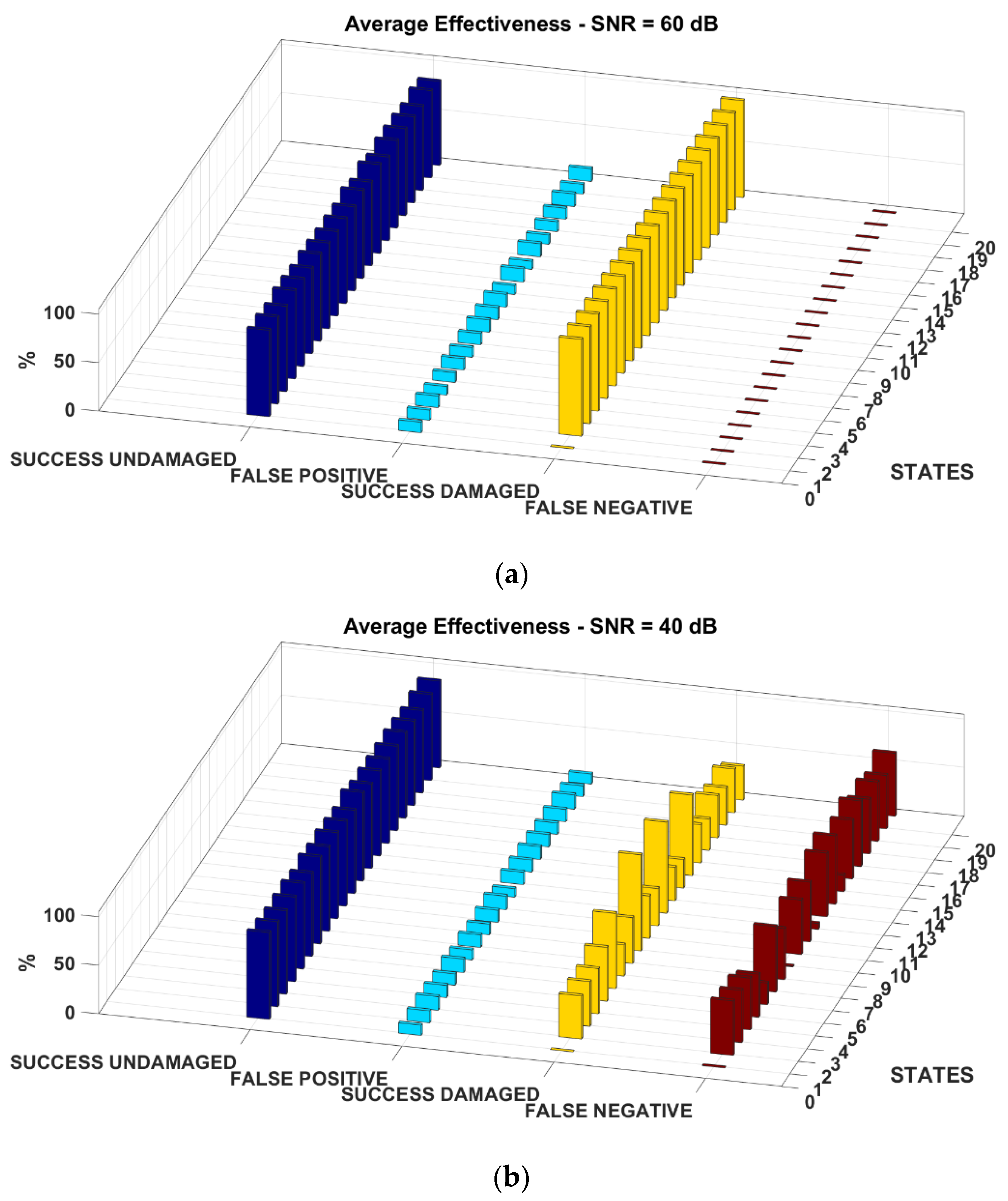
The results for the damage scenarios depicted in Figure 4b are portrayed in Figure 9. Only the 1st mode shape is showed for brevity; the 2nd and 3rd mode shape returned similar results in terms of accuracy (with similar rates of occurrence for both false positives and false negatives). Artificial white Gaussian was added considering SNR = 60 dB and 40 dB.

One can see that the method always successfully labels the undamaged and damaged states correctly for SNR = 60 dB, which is already a relatively large amount of noise.

Note that no damage was inserted in state 00; therefore, no damage was to be identified there, similarly to what expressed for the results of the beam structure (in Figure 6).

The states 01 and 02, which have too small variations of Young’s modulus to be effectively considered as damaged, are rightly identified as false negatives. This proves the reliability of the method in discerning small perturbations, which may happen in real-life acquisitions due to the statistical variance of the acquisitions, from the actual damage. On the other hand, with even more white Gaussian noise artificially added to the input data (SNR = 40), the approach still correctly identifies the undamaged states, while it loses accuracy on the damaged mode shapes of the test set. Specifically, it remains able to recognise the most damaged situations (with a 25% or 50% reduction of Young’s modulus) whenever the damage is inserted at the clamped base. As expected, also by comparison with previous works [10], the scenarios with the damage inserted solely at the mid-length cross-section (states 3 to 5) or on the sides of the base cross-section not fixed to the centre wing box (states 18 to 20).

Regarding the computational efficiency of the algorithm, the whole simulation of the complete HAR wing dataset was performed in around 31 s. The non-optimised MatLab script elapsed on average 2.2 s to perform a single training fold, 3.9 s for CDF validated estimation and 0.02 s for the damage detection task on a single damage state, with no major differences among the 20 states, on an Intel^® Core™ i7-10750H CPU with 2.6 GHz base frequency and 15.8 GB of available RAM. Similar elapsed times were found for the other numerical and experimental cases.

3.3. Results for the Frame FE Model

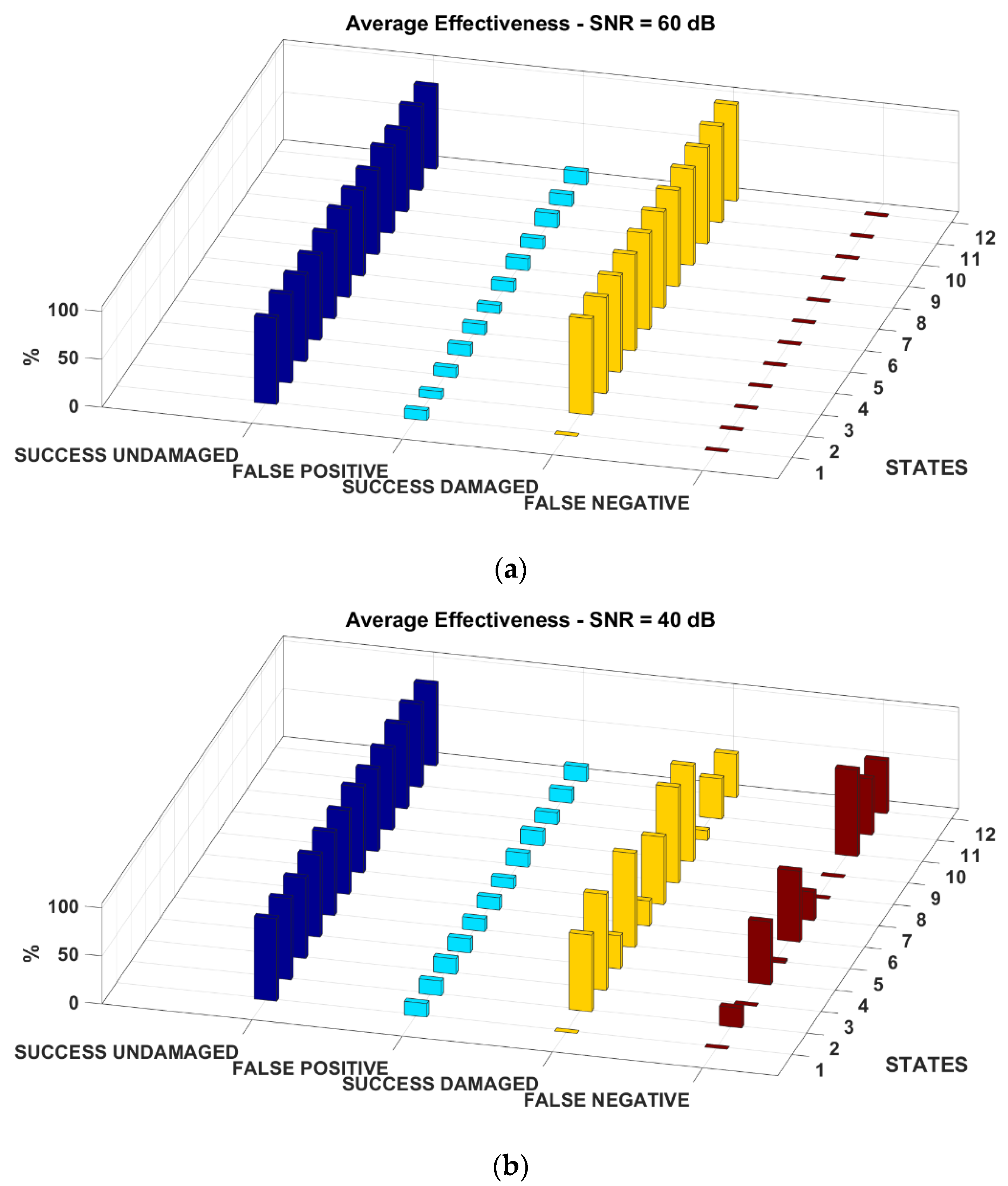
The settings for the second numerical investigation are the same as described in Table 1. Figure 9 reports the results of the frame structure FE model for an increasing level of artificially added noise. Again, as for the previous case studies, consider that no damage was inserted in the baseline (state 1). For what concerns the noise level, the results in Figure 10b show how, for a realistic noisy scenario consistent with current measurement technology, a good performance is reached in the states with high damage severity (stiffness reduction ~75%) or when the damage location is highly influent (states 8 and 9, i.e., with both base columns damaged). Otherwise, Figure 10a shows a high performance level obtained in correspondence of a small noise reduction, achievable with improvement in measurement accuracy or by applying data cleansing and noise reduction techniques. All these findings are consistent with what preliminary assessed in the previous works [28] for the simpler cantilevered beam model.

4. Experimental Validation

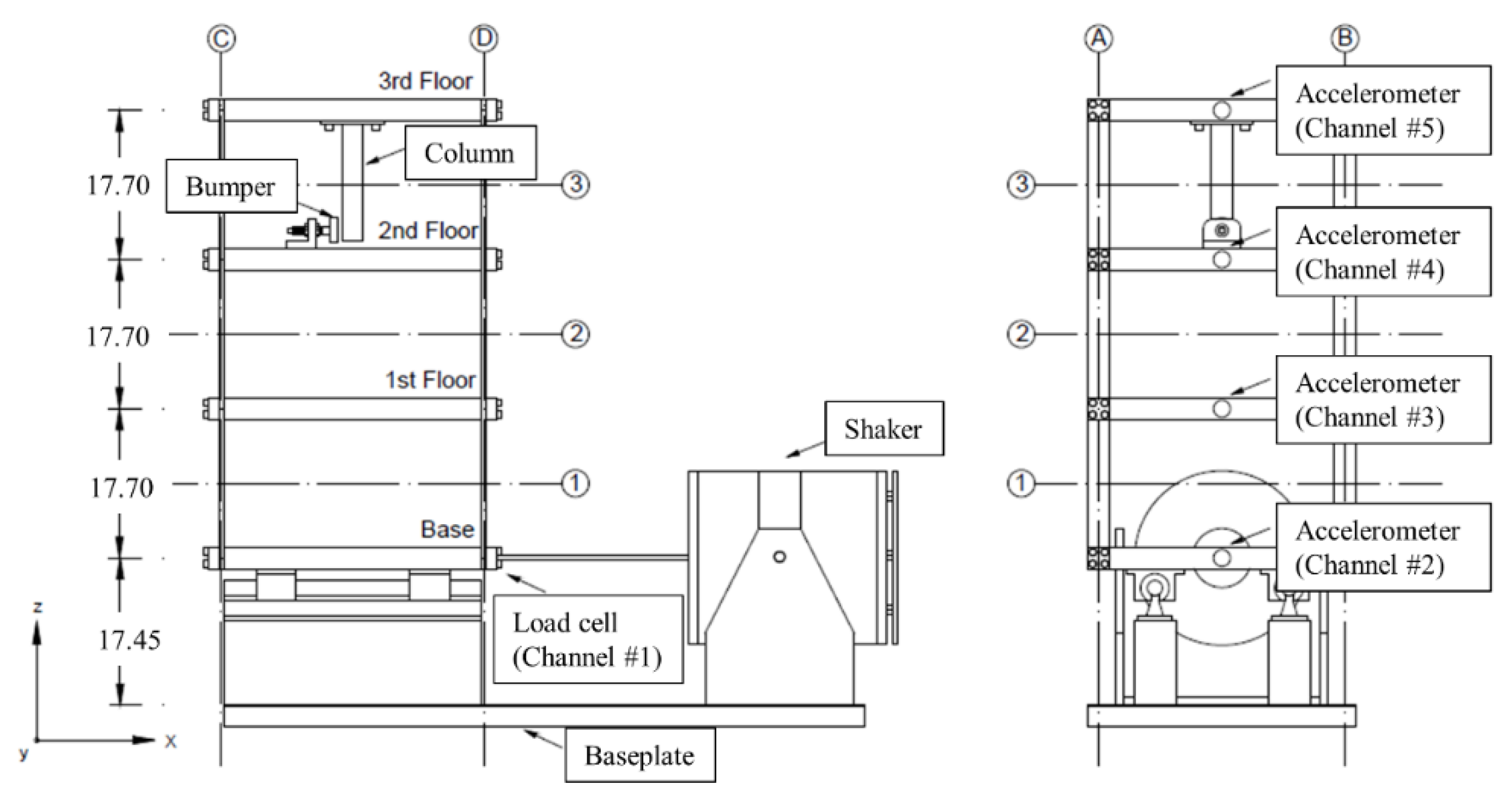
The experimental validation was performed on a well-known database realised at the Los Alamos National Laboratory (LANL). As for the frame numerical model described in the previous Section, the structure (represented in Figure 11) is a three-storey shear-type frame. Seventeen scenarios were considered, as described in

Table 4. Damage States for the Los Alamos National Laboratory (LANL) frame.

	Case	Description
Linear States	1	Undamaged Baseline
	2	Added mass of 1.2 kg at the base
	3	Added mass of 1.2 kg at the 1st floor
	4	87.5% stiffness reduction in one column of the 1st inter-storey
	5	87.5% stiffness reduction in two columns of the 1st inter-storey
	6	87.5% stiffness reduction in one column of the 2nd inter-storey
	7	87.5% stiffness reduction in two columns of the 2nd inter-storey
	8	87.5% stiffness reduction in one column of the 3rd inter-storey
	9	87.5% stiffness reduction in two columns of the 3rd inter-storey
Nonlinear States	10	Distance between bumper and column tip 0.20 mm
	11	Distance between bumper and column tip 0.15 mm
	12	Distance between bumper and column tip 0.13 mm
	13	Distance between bumper and column tip 0.10 mm
	14	Distance between bumper and column tip 0.05 mm
	15	Bumper 0.20 mm from column tip, 1.2 kg added at the base
	16	Bumper 0.20 mm from column tip, 1.2 kg added on the 1st floor
	17	Bumper 0.10 mm from column tip, 1.2 kg added on the 1st floor

. They include one or more stiffness reductions applied to the beams (to simulate damage) and/or one or more added masses (to simulate changing operational conditions). The dataset also included some scenarios with a bumper-column apparatus attached at the top floor. The original intent of this mechanism was to emulate the nonlinear effects induced by a breathing crack [41], which is known to act as a pointwise source of bi-linearity (a deeper discussion can be found in Reference [42]).

Generally, the presence of such nonlinearities is used to detect and localise surface cracks in otherwise linear systems [43]. However, these data are here used with another intent. As it can be noticed from Figure 12c,d, the insertion of the mechanism causes an increase in the system stiffness. Therefore, the natural frequencies grow as well, while a breathing crack would decrease them. However, the bumper-column mechanism affects the mode shapes making them detectable as a deviation from the undamaged baseline. Moreover, since the structural nonlinearities generate noise-like distortions in the frequency response, the damage scenarios 10–17 can be utilised as well to prove the robustness of the procedure when dealing with distorted signals.

The acquisition procedure can be summed up as follows (more details can be found in the original source [44]). Fifty band-limited (20–150 Hz) white Gaussian noise realisations were applied as input for 25.6 s at the structure base. The system response was recorded at four points corresponding to the three levels plus the base, with a sampling frequency $f_s=320$ Hz. The mode shapes were then extracted from the frequency response functions (FRFs) defined between the acceleration output time histories and the force input utilising the FRVF procedure described previously.

Importantly, for states 10–17, the concept of “mode shapes” in a nonlinear context could be not totally accurate. It is necessary to remark that the specific experimental setup (single-input multi-output acquisitions with a random noise as input) only allows linear system identification [45]. The experimental identification of nonlinear normal modes would require more complex procedures which are beyond the objective of this study. Therefore, the extracted mode shapes should be considered as the ones of the underlying linear system for these eight nonlinear states [45].

The Data Augmentation procedure described in Section 2 was applied to increase the number of training and validation data. For illustrative purposes, Figure 13 shows the resulting model obtained by applying the GP Regression over the three mode shapes identified from the experimental data.

The results of the experimental validation are shown in Figure 14. As for all the previous examples, no damage was to be identified in the first state, therefore there are no false alarms nor successful damage identifications. The EFT-based procedure correctly identifies all the structural changes except for the configurations with the bumper-column gap larger than 10 mm and no added mass (i.e., states 10 to 12). However, as it can be seen from Figure 12c, the nonlinear distortions are minimal for this larger gap and the response of the structure is almost indistinguishable from the pristine baseline. The algorithm struggled to recognise the last two states (16 and 17) as well when fed with the first mode shape; this issue did not arise either with the second or the third eigenmode. On the other hand, due to the larger confidence intervals (Figure 13c), the fitting of the third mode shape returned a relatively larger number of false positives (almost constantly 17% for any damage scenario).

5. EFT vs. EVT

To conclude this work, a comparison between the extreme value and the extreme function theory has been performed on all the numerical and experimental data. This comparison can be done directly since the same spatial coordinates were utilised to define all the damaged and undamaged mode shapes. That means that any i-th mode shape is defined on the same n_i points. For EFT, this results in n vectors, which return a single distribution over functions, i.e., 1-dimensional data; while in EVT, there are n_i distributions over scalar values, each one with n samples.

The results are reported in Appendix A (

Table A1. The comparison between Extreme Value Theory (EVT) and EFT for the simply supported beam numerical case study.

BEAM FEM (Hinged-Hinged, SNR = 60 dB)
	FALSE POSITIVE EFT	FALSE POSITIVE EVT	IMPROVEMENT
	[%]	[%]	[%]
Mode Shape #1	6.44	15.53	9.09
Mode Shape #2	9.22	16.87	7.64
Mode Shape #3	4.64	10.76	6.11
BEAM FEM (hinged-hinged, SNR = 40 dB)
	FALSE POSITIVE EFT	FALSE POSITIVE EVT	IMPROVEMENT
	[%]	[%]	[%]
Mode Shape #1	12.04	15.60	3.56
Mode Shape #2	8.40	13.56	5.16
Mode Shape #3	16.07	14.87	−1.20

,

Table A2. The comparison between EVT and EFT for the clamped-hinged beam numerical case study.

BEAM FEM (Clamped-Hinged, SNR = 60 dB)
	FALSE POSITIVE EFT	FALSE POSITIVE EVT	IMPROVEMENT
	[%]	[%]	[%]
Mode Shape #1	6.00	16.62	10.62
Mode Shape #2	8.11	14.40	6.29
Mode Shape #3	1.64	8.82	7.18
BEAM FEM (clamped-hinged, SNR = 40 dB)
	FALSE POSITIVE EFT	FALSE POSITIVE EVT	IMPROVEMENT
	[%]	[%]	[%]
Mode Shape #1	12.91	20.71	7.80
Mode Shape #2	10.60	15.51	4.91
Mode Shape #3	7.40	12.87	5.47

,

Table A3. The comparison between EVT and EFT for the HAR wing spar numerical case study.

HAR FEM (SNR = 60 dB)
	FALSE POSITIVE EFT	FALSE POSITIVE EVT	IMPROVEMENT
	[%]	[%]	[%]
Mode Shape #1	11.26	19.28	8.02
Mode Shape #2	7.6	14.96	7.36
Mode Shape #3	9.56	16.16	6.6
HAR FEM (SNR = 40 dB)
	FALSE POSITIVE EFT	FALSE POSITIVE EVT	IMPROVEMENT
	[%]	[%]	[%]
Mode Shape #1	12.32	28.04	15.72
Mode Shape #2	10.42	23.02	12.6
Mode Shape #3	11.52	26.28	14.76

,

Table A4. The comparison between EVT and EFT for the shear-type frame numerical case study.

FRAME FEM (SNR = 60 dB)
	FALSE POSITIVE EFT	FALSE POSITIVE EVT	IMPROVEMENT
	[%]	[%]	[%]
Mode Shape #1	11.19	20.49	9.30
Mode Shape #2	8.81	15.81	7.00
Mode Shape #3	12.24	13.78	1.56
FRAME FEM (SNR = 40 dB)
	FALSE POSITIVE EFT	FALSE POSITIVE EVT	IMPROVEMENT
	[%]	[%]	[%]
Mode Shape #1	14.06	20.28	6.22
Mode Shape #2	7.06	10.70	3.64
Mode Shape #3	14.97	22.66	7.69

and

Table A5. The comparison between EVT and EFT for the experimental case study.

FRAME EXPERIMENTAL
	FALSE POSITIVE EFT	FALSE POSITIVE EVT	IMPROVEMENT
	[%]	[%]	[%]
Mode Shape #1	1.25	3.08	1.83
Mode Shape #2	0.43	2.50	2.07
Mode Shape #3	10.38	17.55	7.16

) for all the numerical and the experimental case studies presented in the previous Sections (in the same order). Everywhere, the increment is calculated as FALSE POSITIVE EVT—FALSE POSITIVE EFT, expressed in percentage.

As expected, the incidence of false positives decreased significantly, with an improvement everywhere larger than 6% for the HAR spar Finite Element Model (even with a double-digit increment in the false alarm reduction for the case with SNR = 40 dB) and still very relevant for the second numerical case study. The EVT outperformed the EFT in terms of fewer false positives only for the simply supported beam and for the third mode shape with the lowest SNR. This is most probably due to the combination of the larger confidence intervals of the GP regression over the 3rd mode shape, the larger variability induced by the noise, and the structural symmetry. The experimental data confirmed the key findings encountered on the simulated dataset. Specifically, the percentage of false positives decreased for all the three mode shapes.

6. Conclusions

This study investigated the validity of EFT as a framework for mode shape-based SHM in 2-dimensional plate-like and frame structures, which are representative of common applications in Aerospace and Civil Engineering, respectively. The rationale is that damage is a rare occurrence and therefore the data-driven models defined over the undamaged conditions must take this consideration into account. Experimental and numerical data were utilised to this aim for different damage locations and severity levels. The robustness of the procedure to artificially added white Gaussian noise has been methodically studied and the results have been benchmarked against the results of the same algorithm trained with pointwise EVT values, showing a statistically relevant decrease of the number of false positives. Moreover, the use of EFT allows to compare points where the data were not directly collected; furthermore, it assigns only one possible outcome (“normal” or “abnormal”) to the whole function. On the other hand, the single components of the mode shape, if taken one by one as in the EVT, could be under the threshold at some modal coordinates and over it at other locations for the same identification.

This study provides a strong foundation for future works in the field of EFT and EVT for structural health monitoring purposes. It will be important to validate the proposed approach in situ on real-life civil structures. Another related field of research, which the Authors are intended to investigate deeper in the next future, regards the scarcity of data from damaged structures and the need to compensate with numerically simulated data.