Determination of the Crack Propagation Direction in Mixed-Mode Missions due to Cyclic Loading

Abstract

The evaluation of cyclic crack propagation due to missions with varying mixed-mode conditions is an important topic in industrial applications. This paper focuses on the determination of the resulting propagation direction. Two criteria are analyzed, the dominant step criterion and the averaged angle criterion, and compared with experimental data from tension-torsion tests with and without phase shift. The comparison shows that the dominant step criterion yields better results for small to moderate values of the phase shift. For a large phase shift of 90°, the experimental results are not very consistent, and therefore, no decisive conclusions can be drawn.

1. Introduction

In aircraft engine components, the accurate prediction of the propagation of potential cracks has gained much importance in recent decades. Indeed, due to challenging requirements related to fuel consumption and (consequently) weight, traditional crack initiation criteria have been replaced by damage tolerance concepts [1]. Not only life prediction in terms of the number of cycles is crucial, but also the accurate prediction of the crack propagation direction is a target. This applies for instance to blisks, in which a crack initiated in the blade due to vibrations may (depending on the crack propagation direction) grow into the disk and lead to a catastrophic failure due to the centrifugal loading [2]. Therefore, both the crack propagation rate and direction are essential information.

Due to the different time constants involved in mechanical and thermal processes, the stress and temperature evolution during flight are quite different, and up to a few hundred loading steps may be needed to accurately simulate all conditions. At any location along a potential crack, this leads to exactly the same amount of different mixed-mode states. Due to small-scale plasticity at the crack tip, a linear elastic stress intensity approach can be taken. For each of the stress states separately, one can determine the crack propagation speed and direction [3,4]. The question is, however, how to determine the speed and direction due to the complete mission. For the speed, a cycle extraction through a rainflow algorithm [5] is the usual way to go. Still, the rainflow algorithm is usually applied to a one-dimensional function, and in mixed-mode transient temperature conditions, it is not necessarily clear what function should be taken. For the crack propagation direction, the fundamental question is how to arrive at the propagation direction for the complete mission. This paper concentrates on the latter aspect.

For monotonic plane mixed-mode loading, different stress or energy based fracture criteria have been developed and adapted since the 1960s in the scope of linear elastic fracture mechanics (LEFM). In this context, the maximum tangential stress criterion (MTS) of Erdogan and Sih [6], the maximum shear stress criterion (MSS) [7,8], and, for example, the equivalent stress intensity factor $K_v$ of Richard et al. [3,9] should be mentioned. For the case of a general three-dimensional mixed-mode loading, Schöllmann et al. [10] developed the so-called ${\sigma }_1^{\prime }$-criterion based on the MTS criterion. Furthermore, the empirical criterion according to Richard et al. [9] represents an extension from the 2D to the 3D state and stands out especially because of its easy adaptability to experimental results. Finally, a general approach based on the principal planes of the asymptotic stress tensor at the crack tip was developed by Dhondt [11] and applied in several subsequent publications [2,12].

As proven by Yokobori et al. [13], Tong et al. [14], and Magill and Zwerneman [15], among others, all criteria for monotonic loading can in principle also be applied to fatigue crack growth under proportional loading. However, in the case of non-proportional mixed-mode loading, the fracture criteria developed for monotic and cyclic proportional loading are no longer applicable. This circumstance essentially results from the fact that the time-varying stress path can no longer be described by only one parameter. A non-proportional loading occurs, for example, by the superposition of a static load component with a cyclic load component and has been studied by [2,16,17,18,19,20,21,22], among others. Mode II or mixed-mode overloads interspersed in a Mode I basic stress can be considered as a special case of a non-proportional mixed-mode loading, as studied for example by Sander and Richard [23,24], as well as by Eberlein and Richard [25]. The general case of non-proportional loading is represented by phase-shifted mixed-mode loading, which was the focus of investigations in [26,27,28,29].

Based on the experimental investigations of Brüning [30], Yang [31] carried out extensive finite element analyses, as well as crack propagation analyses in the context of LEFM. However, no unified criterion for determining the crack propagation direction could be found here, since the mixed-mode relationship also changes continuously with the crack growth.

In particular, with regard to the superposition of all three crack modes, very few investigations exist for phase-shifted mixed-mode loading [32,33]. Furthermore, a special problem in the case of three-dimensional mixed-mode loading is the geometry-dependent coupling of Mode II and Mode III at the surface, which was demonstrated, for example, in [34,35,36]. However, this is currently not generally taken into account in the crack propagation concepts developed or in the determination of the crack growth curves.

One way of arriving at a propagation deflection angle for the complete mission is to start from the deflection angles calculated for each loading step separately, assuming each step to be the extremal value of a zero-max cycle by simply adding zero as the second entry in the cycle (a zero-max cycle is a cycle in which one of both K-values is zero). The problem is how to combine the individual step angles. One obvious way is to proceed as in BEASY [37] and to calculate the mission deflection angle as a weighted average of the deflection angles in the individual steps. For the weight, the equivalent K-factor in each individual step is used. Alternatively, one could use a dominant step criterion. Such a criterion postulates that the deflection angle of the mission is the same as the deflection angle of the dominant step. In [2], the dominant step was defined as the step with the highest crack propagation rate obtained by substituting the equivalent K-factor in a Paris-type crack propagation law.

In the present publication, the weighted deflection angle criterion is compared with the dominant step criterion. To this end, the former criterion, as defined in [37], is slightly modified. Indeed, to take the temperature effect into account, the weight in each loading step is taken to be the crack propagation rate obtained by substituting the equivalent K-factor into a simple Paris-type law (this is similar to the way the dominant step is identified in the dominant step approach). In this way, the temperature enters the calculation through the temperature-dependent constants in the Paris law. The dominant step criterion is kept in the form already used to analyze cruciform specimens in [2]. Both criteria are validated using tension-torsion test results with and without phase shift [38]. It must be emphasized that since the tension-torsion tests are isothermal, only the way both criteria handle the change of mode-mixity in a mission is validated and not the way the temperature is taken into account.

The next section describes the experimental setup. Then, a detailed description of the crack propagation procedure for mixed-mode missions in CRACKTRACER3D is given. Finally, the validation of the crack propagation criteria using the tension-torsion results is described, and the most appropriate criterion is identified. A list of the nomenclature used throughout the article is given in

Table 1. Nomenclature.

Symbol	Meaning
$A_i$	area of triangle i
$a_{surf}$	crack length measured on the specimen free surface
$d_{ax}$	distance in the axial direction
$da/dN$	crack propagation rate
${(da/dN)}_{ref}$	Paris law constant
$f_C$	critical correction
$f_{th}$	threshold correction
$f_R$	R-value correction
F	axial force
$K_C$	critical value
$K_{eq}$	equivalent stress intensity factor
$K_I$	Mode I stress intensity factor
$K_{II}$	Mode II stress intensity factor
$K_{III}$	Mode III stress intensity factor
m	Paris law exponent
$M_t$	torsional moment
$N_{step}$	number of steps in the mission
r	radial polar coordinate at the crack tip
R	$K_{min}/K_{max}$
$R_{axial}$	$F_{min,axial}/F_{max,axial}$
$R_{p0.2}$	yield strength
$R_{torsion}$	$M_{t,min}/M_{t,max}$
T	temperature
$V_i$	volume of the triangular prism built on $A_i$
x	Cartesian coordinate at the crack tip in the propagation direction
y	normal Cartesian coordinate at the crack tip
z	tangential Cartesian coordinate at the crack tip
$\mathsf{\Delta }a$	crack increment
$\mathsf{\Delta }{K}_{eq}$	equivalent stress intensity factor range
$\mathsf{\Delta }{K}_{ref}$	Paris law constant
$\mathsf{\Delta }{K}_{th}$	threshold value
$\mathsf{\Delta }\phi$	error in the deflection angle
${\sigma }_N$	max nominal axial stress
${\sigma }^{*}$	self-similar stress tensor
${\tau }_N$	max nominal torsional stress
$\phi$	angular polar coordinate at the crack tip
	deflection angle
${\phi }_o$	polar angle made by the highest self-similar principal stress plane
$\psi$	twist angle

.

2. Crack Propagation in Tension-Torsion Tests: Experimental Setup

The experiments under superimposed cyclic tension-compression and torsional loading were carried out with specimens made of the high-strength steel 34CrNiMo6 in quenched and tempered conditions. To avoid additional influences due to the rolling direction, the corresponding flat specimens were made from a forged ingot with the chemical composition shown in

Table 2. Chemical composition (in % of weight) of the tested material 34CrNiMo6 [39].

Element	C	Mn	Si	P	S	Cr	Mo	Ni	Al
Composition	0.36	0.73	0.26	0.006	0.001	1.57	0.22	1.57	0.022

and the mechanical properties given in

Table 3. Mechanical properties of the tested material 34CrNiMo6 [39].

${\mathit{R}}_{\mathit{p}0.2}$ (MPa)	${\mathit{R}}_{\mathit{m}}$ (MPa)	${\mathit{A}}_5$ (%)	Hardness (HB)	E (MPa)	$\mathit{\nu }$
819	963	15	326	210,000	0.3

.

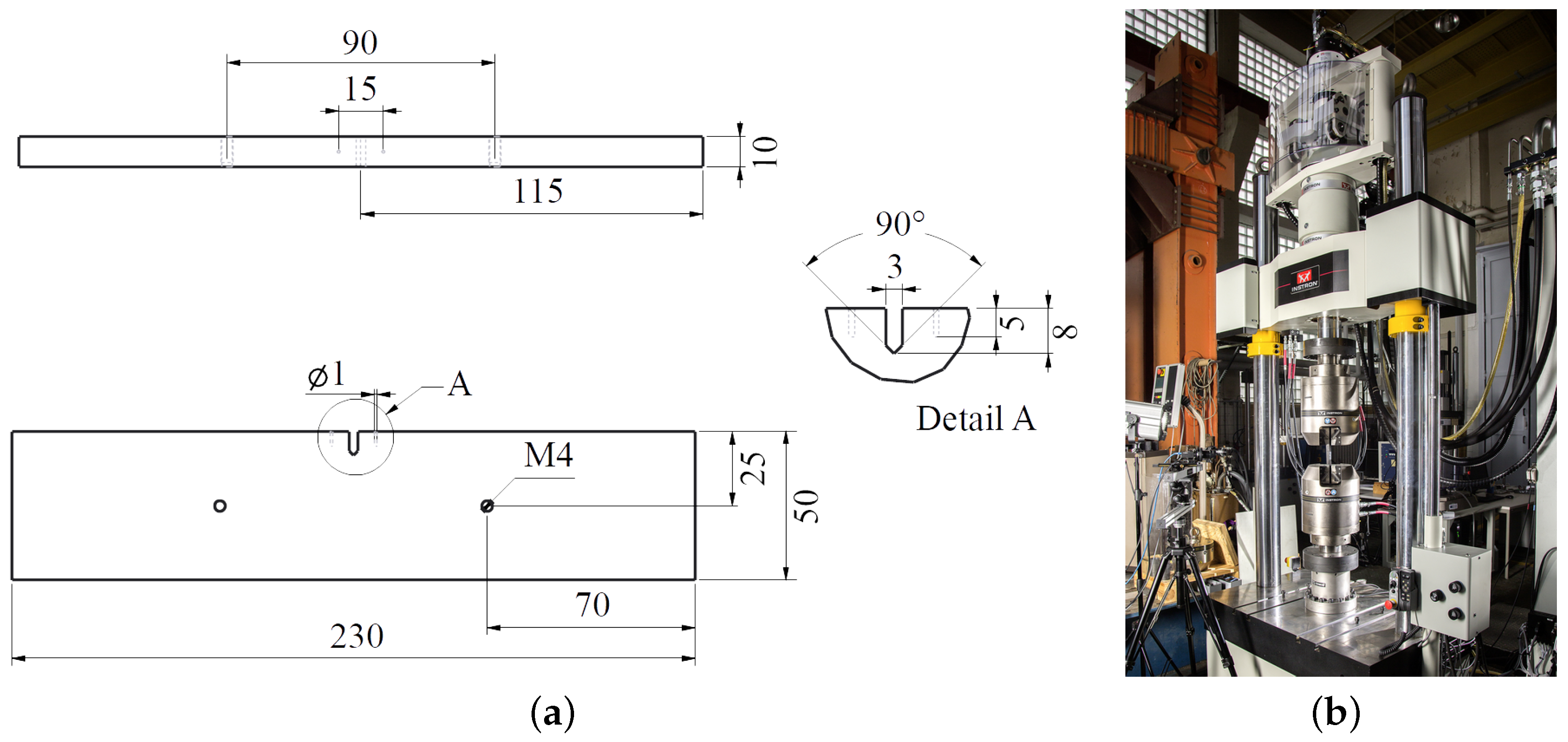
Single-edge notched-tension-compression specimens (SEN-TC) with a length of 230 mm, a width of 50 mm, and a thickness of 10 mm were used (Figure 1a). Under the superimposed loading condition, these specimens’ shape guarantees the presence of all three crack modes along the crack front. Furthermore, the SEN specimen also allows for a good observation of the crack propagation on the surfaces.

To create comparable and reproducible conditions, the specimens were provided with a sharp V-shaped starter notch by wire erosion (see the detail in Figure 1a). In addition, initiation of a Mode I controlled fatigue crack was performed at a tension-compression load of ±25 kN with $R_{axial}=-1$ until a crack increment of $\mathsf{\Delta }a=0.3$ mm was reached. For this purpose, the potential drop technique with the appropriate measuring device (MATELECT [41]) was used, whereby the crack increment to be achieved corresponded to a 2% change in the electrical potential. Both the initiation of the cracks and the experimental tests were performed on a servo-hydraulic tension/torsion testing machine (Figure 1b), with which axial loads up to ±250 kN and torsional moments up to ±2 kNm can be realized.

Regarding the determination of the superimposed tension-compression and torsional loading, at first, a fixed load level for the axial loading was defined. In detail, this level is described by the quotient of the maximum nominal axial stress ${\sigma }_N$ to the yield strength $R_{p0.2}$ for 0.2% plastic strain of the material (Table 3) and amounts to ${\sigma }_N/R_{p0.2}=0.07$. 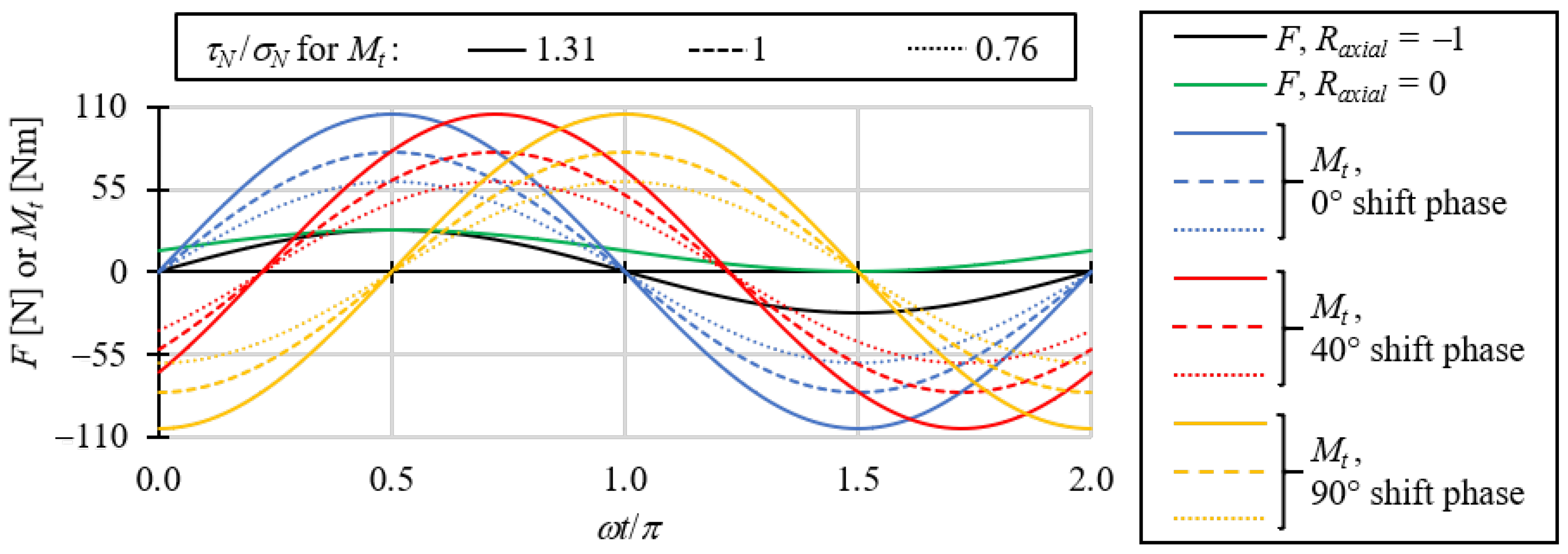This results in a maximum load amplitude of the axial force of F = 27.5 kN. In addition, three different loading type ratios were selected, which result from the quotient of the maximum nominal torsional stress ${\tau }_N$ to the maximum nominal axial stress ${\sigma }_N$ in the undisturbed cross-section: ${\tau }_N/{\sigma }_N=0.76$, 1, and 1.31. Since the axial load level remained constant at the start of all tests, the maximum torsional moments $M_t=60.5$ Nm, 80 Nm, and 104.75 Nm were applied to realize the three ${\tau }_N/{\sigma }_N$ ratios.

Furthermore, the influence of the stress ratio of the axial load on the crack propagation behavior under mixed-mode conditions was investigated. For this purpose, tests were carried out both at $R_{axial}=0$ and $R_{axial}=-1$. The stress ratio of cyclic alternating torsion was $R_{torsion}=-1$ in all experiments.

In order to investigate the influence of a non-proportional mixed-mode load on the fatigue crack propagation, the torsional moment was set in-phase to the tension-compression load, as well as phase shifted by 40° and 90° to the axial loading. In total, there were eighteen different load cases, which result from the superposition of an axial load with a torsional moment from the schematic diagram for one load cycle in Figure 2.

All experiments were performed load controlled at room temperature. A change of the twisting angle of the torsion cylinder by more than 1° was considered to be the termination criterion.

3. Crack Propagation Procedure in CRACKTRACER3D

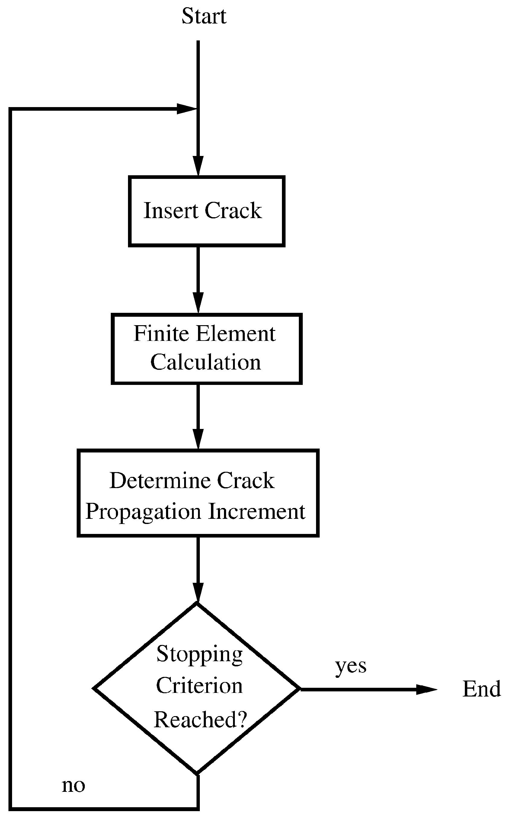
For the validation, the test results were simulated by performing cyclic crack propagation calculations using the MTU in-house software CRACKTRACER3D. This is a fully automatic cyclic crack propagation tool using the finite element method. A calculation based on CRACKTRACER3D consists of several increments. Each increment is made up of a pre-processing part, a finite element call, and a post-processing part (Figure 3). Let us for the sake of clarity at first assume that there is only one loading step.

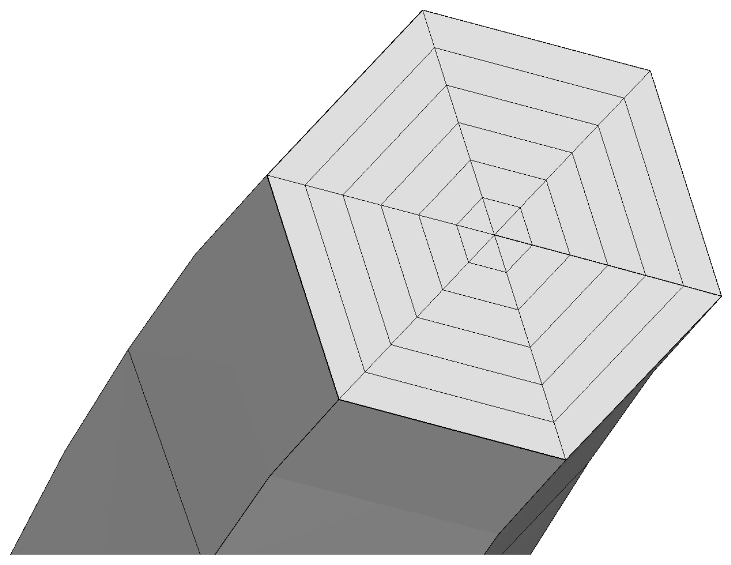
The input for the pre-processor consists of a finite element input file for the uncracked structure (including the mesh, the boundary conditions, the loading, etc.) and a file containing the actual crack geometry. The pre-processor inserts this crack into the mesh and generates a finite element deck for the cracked structure. It does so by remeshing a part of the mesh in which crack propagation is supposed to take place (the so-called domain). This domain is remeshed using quadratic hexahedral elements with reduced integration in a flexible cylinder with a hexagonal cross-section surrounding the crack front (the so-called tube) and quadratic tetrahedral elements elsewhere. All meshes were connected using linear multiple point constraints. 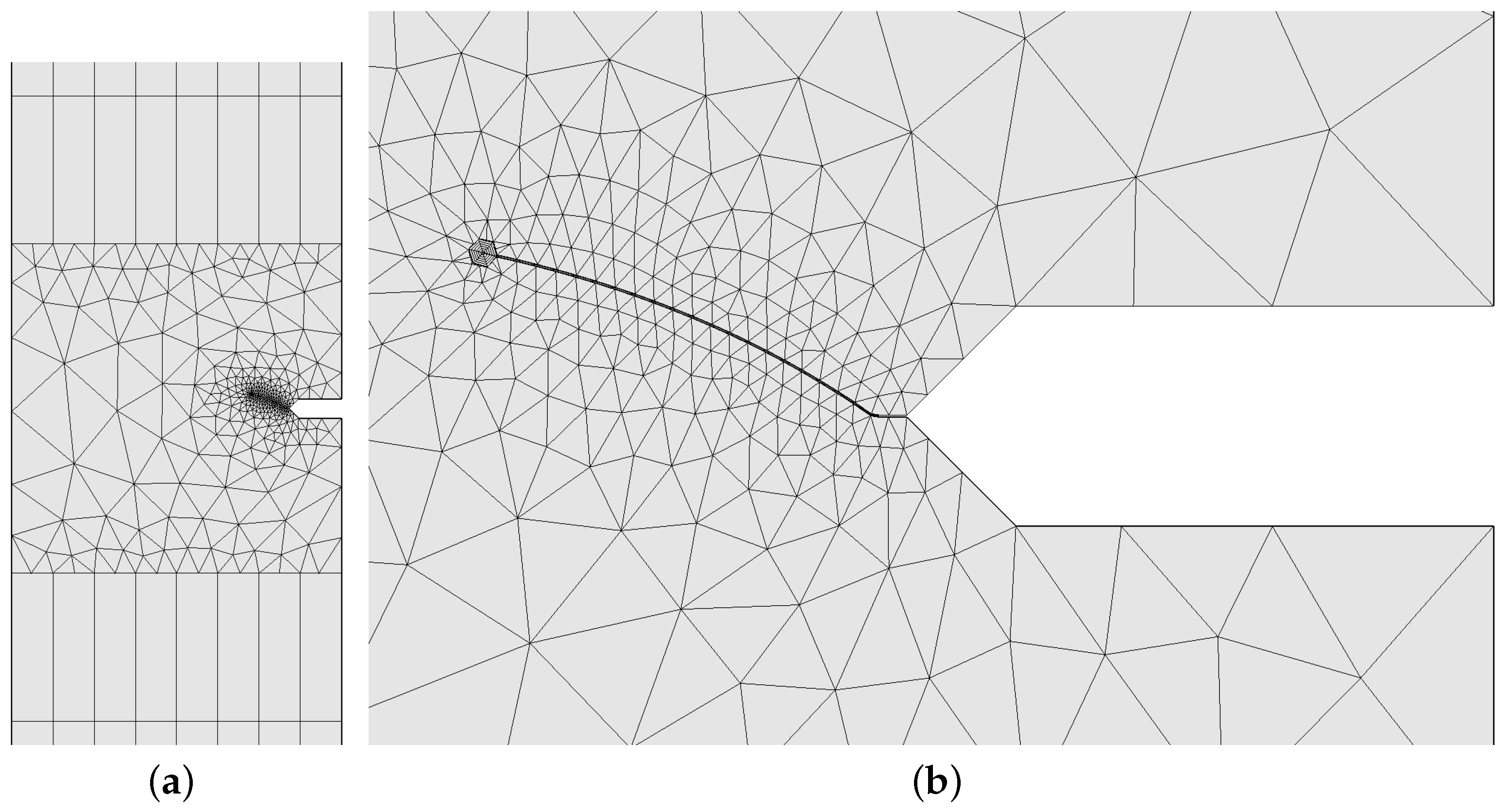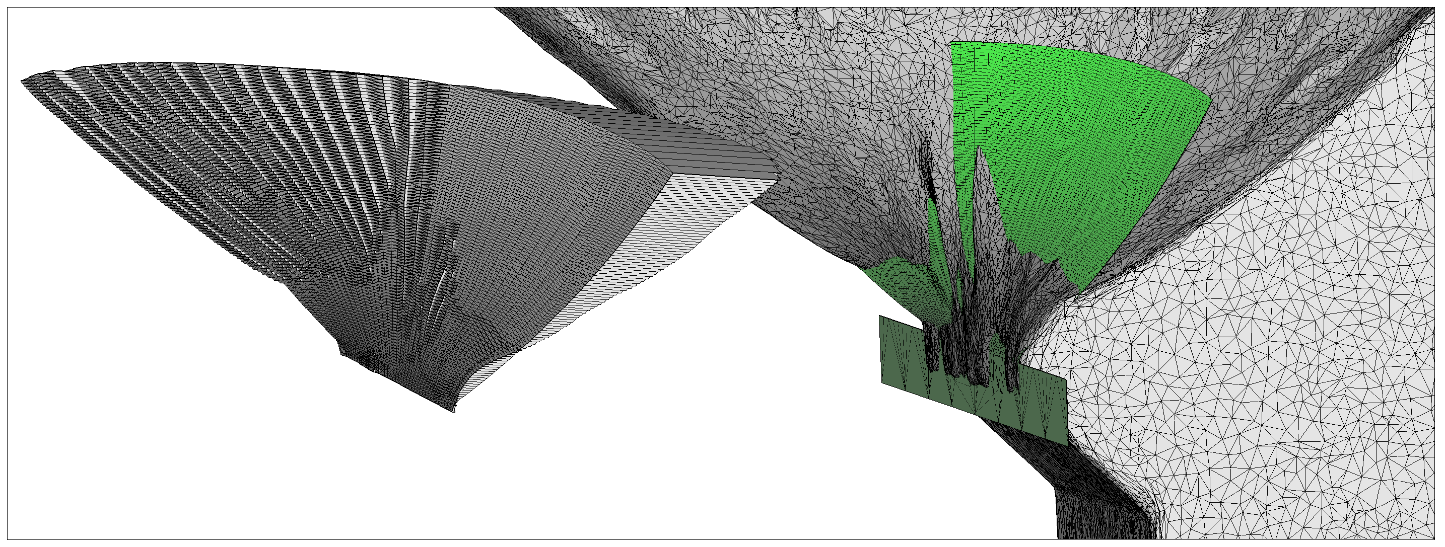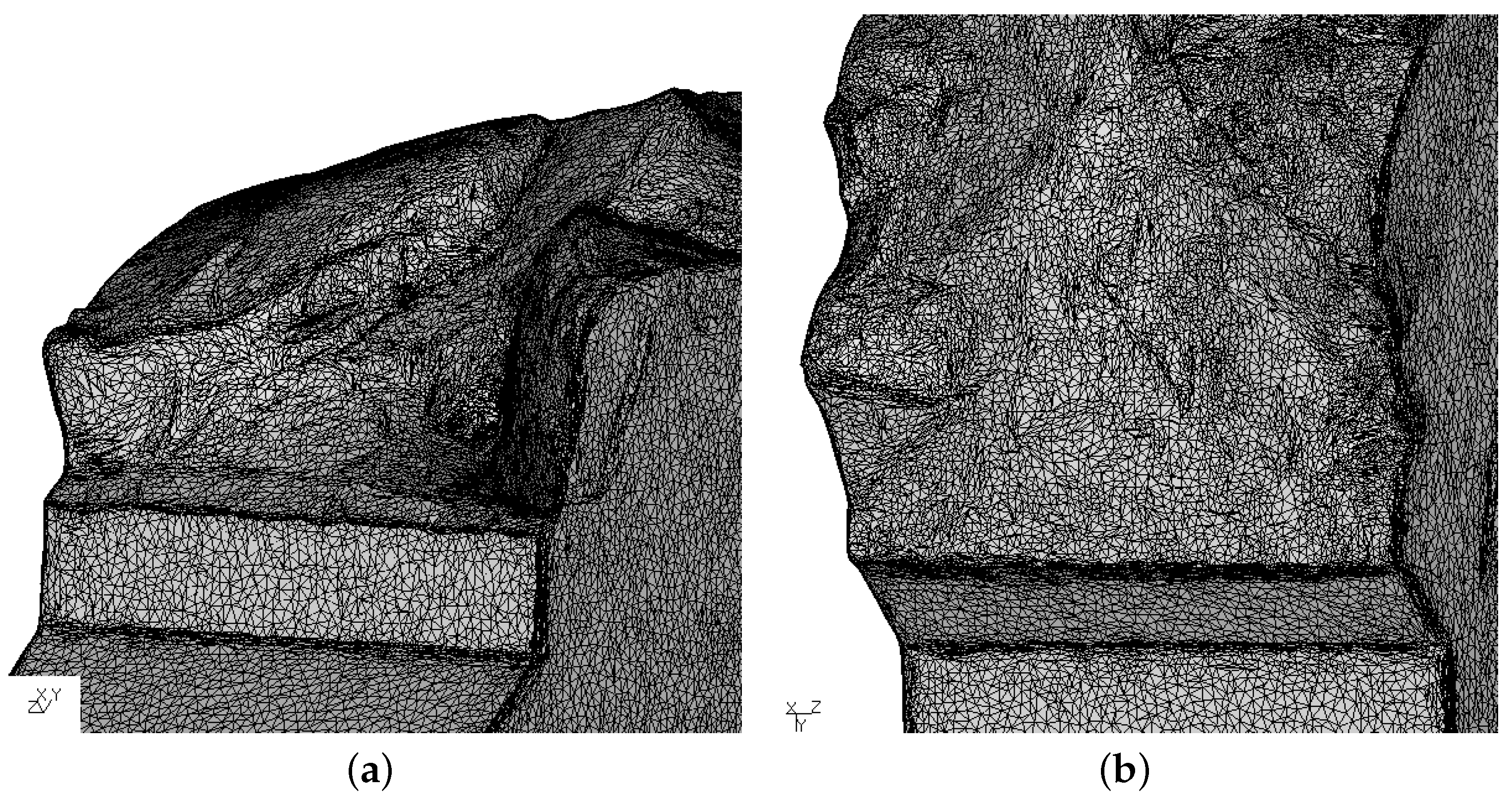Figure 4 shows a typical mesh during crack propagation in the tension-torsion specimen. In Part (a) of the figure, one notices the original mesh (quadratic hexahedral elements in this case) on the top and bottom. The middle part is the domain, which is primarily meshed with tetrahedral elements. At the crack front, in a hexagonal cylinder, twenty-node brick elements with reduced integration were used (Figure 5). Barlow [42] proved that the integration points of these elements are superconvergent, i.e., the stresses in these integration points have also a quadratic accuracy.

The innermost layer of hexahedral elements adjacent to the crack front are so-called collapsed quarter-point elements [43,44]. These are regular 20-node brick elements, one face of which is collapsed to a line. The 8 nodes in this face are reduced to 3, i.e., one and the same node may occur more than once in the element topology. Furthermore, mid-nodes on edges having one node in common with the crack front are moved into a quarter-point position. It has been proven that these elements exhibit the $1/\sqrt{r}$ singularity typical for the stress and strain field at the crack tip in linear elastic calculations.

After the creation of the new mesh, any boundary conditions applied to the domain were appropriately modified. Subsequently, a linear elastic finite element calculation was performed with the free software finite element tool CalculiX [45]. As a result of the calculation, the stresses at the reduced integration points in the 20-node collapsed hexahedral elements were stored in a file.

The post-processor uses these stresses to obtain the K-factors (stress intensity factors) along the crack front. To this end, the stress obtained by the finite element method was compared to the asymptotic stress field at the crack front. For isotropic materials, this latter field is analytically available [46] and takes the form:

$${\sigma }_{xx}=\frac{1}{\sqrt{r}}{f}_{xx}(\phi ,K_I,K_{II},K_{III}),$$

(1)

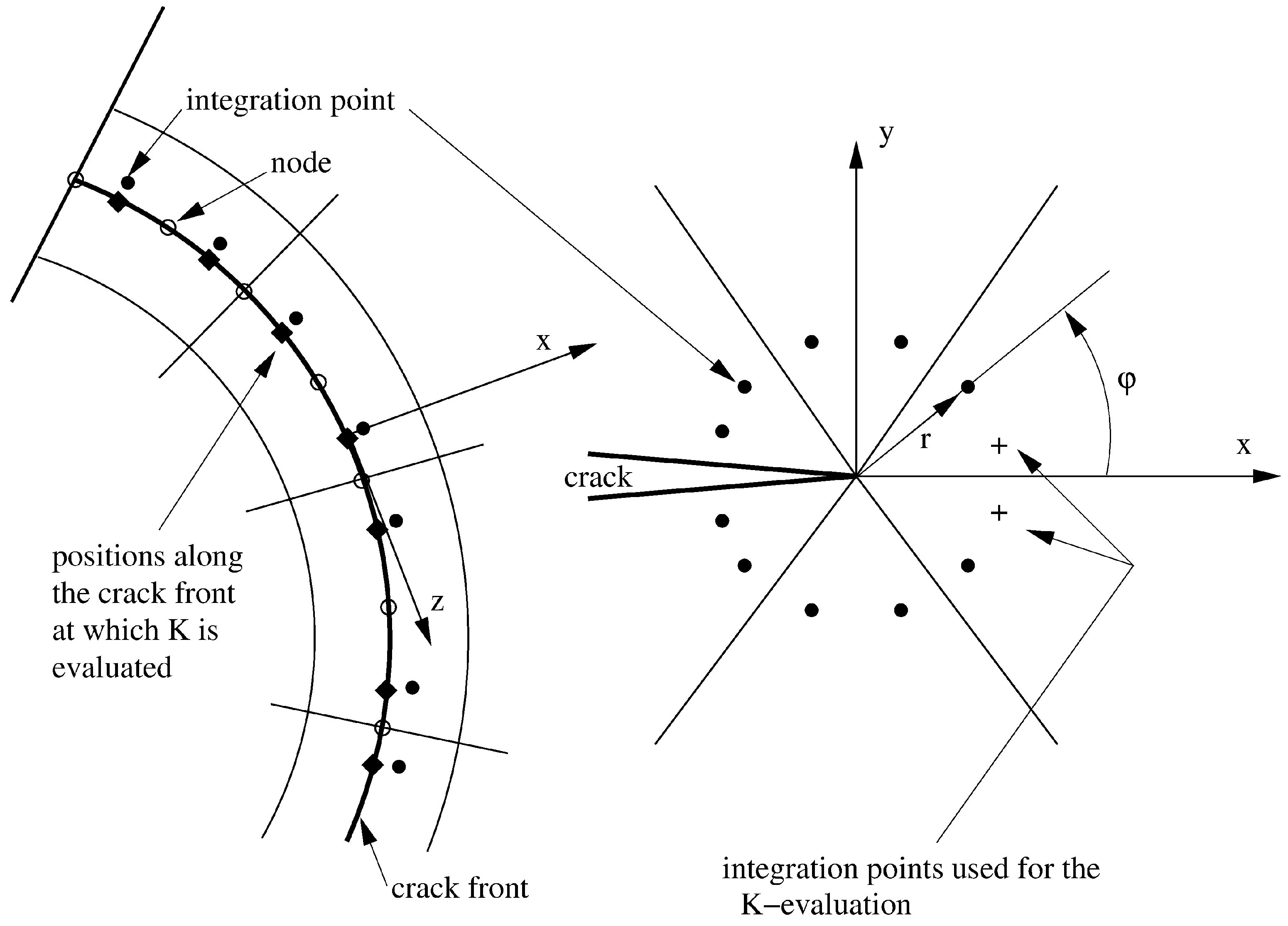
and similar for the other stress components. Here, the x-y-z coordinate system is a local coordinate system at the crack front: the y-axis is locally orthogonal to the crack plane; the x-axis is in the local crack plane and locally orthogonal to the crack front in the direction of the propagation; the z-axis forms a positive coordinate system with the x and y-axis; see Figure 6. The left part of the figure gives a view of the crack plane. It shows the elements immediately adjacent to the crack front and the closest integration points ahead of the crack front (in the direction of the positive x-axis). Since the reduced integration point scheme in a 20-node brick element is a 2 × 2 × 2 scheme, there are two integration points along and ahead of the crack front at locations $\pm \frac{1}{\sqrt{3}}$ in a local coordinate range extending from −1 to 1. The right part is a cut parallel to the x-y plane. It shows the 6 collapsed quarter point elements containing the crack and the closest integration points to the front. Each integration point is characterized by specific values for r and $\phi$, where r and $\phi$ are cylindrical coordinates in the x-y plane.

At any location of the integration points along the crack front (symbolized by diamonds in Figure 6), e.g., at the location of the local axes in the left of Figure 6, any of the integration points on the right of the figure can be used to obtain the K-values at that location. Indeed, in each integration point, the finite element calculation yields 6 stress components, leading to 6 equations of the type in Equation (1) in the 3 unknown K-factors (r and $\phi$ are known for the integration point). However, a detailed analysis showed that not all integration points were equally accurate. More precisely, the integration points immediately ahead of the crack front and labeled by a + sign on the right of Figure 6 were most accurate. Furthermore, it proved advantageous to discard the use of the equation for ${\sigma }_{zz}$, to avoid the problem of whether plane stress or plane strain applies at the actual crack location (the asymptotic expression for ${\sigma }_{zz}$ is different for plane stress and plane strain). Therefore, we ended up with 5 equations in 3 unknowns for each of the locations marked with a +. Using the least squares method, this yielded a triple of K-values for the integration point at positive y and a triple for the integration point at negative y. Taking the mean yielded the final values for $K_I,K_{II},K_{III}$ at that crack front location. Acting in a similar way, the K-values can be obtained for all integration point locations along the crack front. To obtain the values at the nodes, linear interpolation along the crack front was applied. At the free surface, however, extrapolation was used. For a comparison for simple examples of the present method with other methods to determine the K-values, the reader is referred to [47].

Now, the K-values $K_I,K_{II},K_{III}$ were determined at any nodal location along the crack front. The aim was to obtain a crack propagation increment. To this end, the K-triple was transformed into an equivalent K-factor $K_{eq}$, which can be used in an appropriate crack propagation law. Furthermore, the crack propagation direction had to be determined, characterized by a deflection angle $\phi$ and a twist angle $\psi$. These values can be found by postulating that the crack propagation will take place in a plane orthogonal to the largest principal self-similar stress such that the crack tip is contained in this plane. The self-similar stress is defined as the asymptotic stress multiplied by $\sqrt{r}$. To explain this in more detail, let us have a look again at Equation (1). Now, $K_I,K_{II}$ and $K_{III}$ are known. The resulting asymptotic stress field is clearly a function of r and $\phi$. The dependency on r, however, is common to all stress components, so we can discard it. This leads to the self-similar stress ${\sigma }^{*}$ with components:

$${\sigma }_{xx}^{*}=f_{xx}(\phi ,K_I,K_{II},K_{III}),$$

(2)

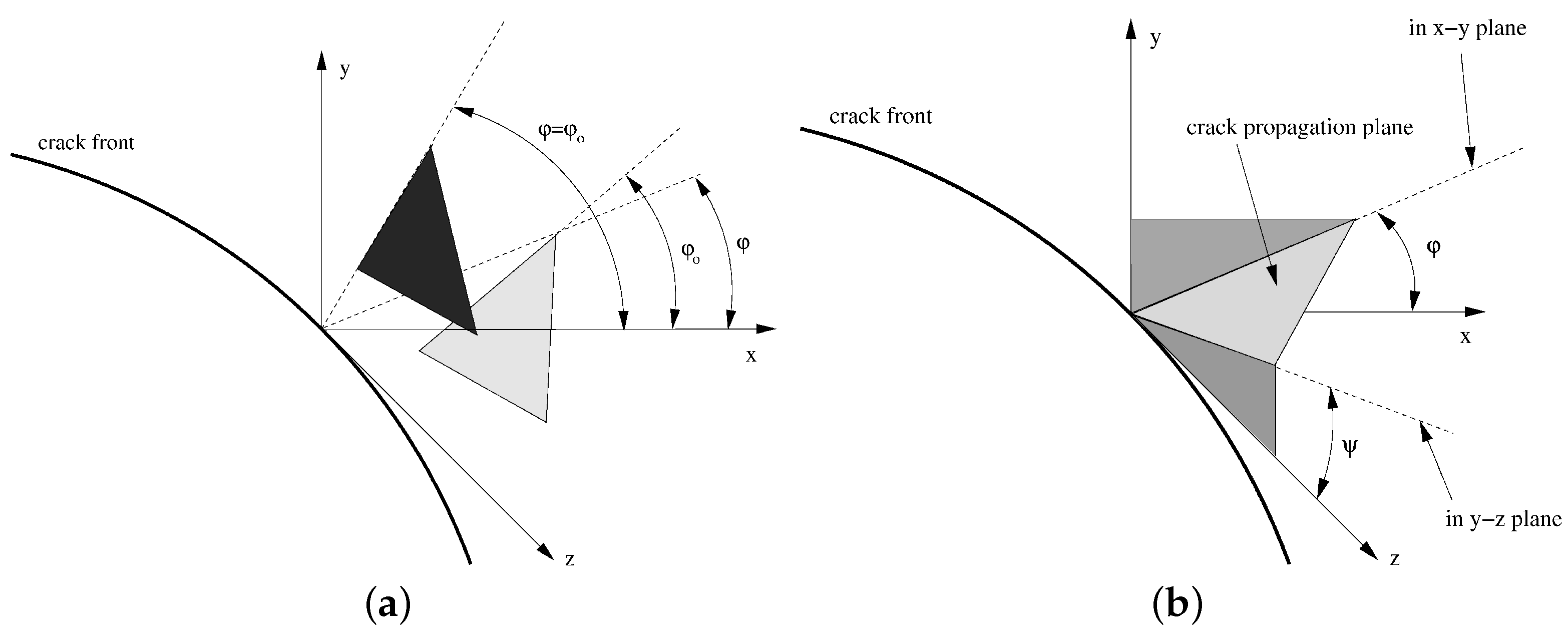
and similar for the other terms. The only variable left here is $\phi$. For a fixed value of $\phi$, the principal values and directions for this tensor can be determined. Let us assume that the cross-section of the principal plane (symbolized by the light gray triangle in Figure 7a) corresponding to the largest self-similar principal stress with the local x-y plane makes an angle with the x-axis of ${\phi }_o$. If $\phi \ne {\phi }_o$, this line does not go through the crack tip and cannot be a crack propagation direction. By varying $\phi$ between −90° and 90° until a value is found for which $\phi ={\phi }_o$, the crack propagation direction is found (symbolized by the black triangle in the figure). If more than one such value is found, the one corresponding to the largest self-similar stress value is taken. Once the correct value for $\phi$ is determined, the equivalent K-value $K_{eq}$ corresponds to the eigenvalue and the twist angle $\psi$ to the angle that the cross-section of the principal plane with the y-z plane makes with the z-axis (cf. Figure 7b). The deflection angle corresponds to $\phi$. The criterion discussed here is straightforward and clearly relies on physical principles. The results were very similar to other criteria such as the criterion by Richard [3], and a comparison with that criterion can be found in [11].

By the use of $K_{eq}$, $\phi$, and $\psi$, the crack propagation increment can be determined. The size of the increment is obtained by substituting $\mathsf{\Delta }K=K_{eq}$ into a crack propagation law (since right now, there was only one loading step, a 0-max cycle was assumed; the extension to several loading steps follows later in the article). Here, the crack propagation law discussed in [48] was used. It is a multiplicative law separating the Paris, threshold, and critical range in the form:

$$\frac{da}{dN}=\left[{\left(\frac{da}{dN}\right)}_{ref}{\left(\frac{\mathsf{\Delta }K}{\mathsf{\Delta }{K}_{ref}}\right)}^m\right]\frac{f_R·f_{th}}{f_c},$$

(3)

where the Paris range is in square brackets. One of the parameters ${\left(\frac{da}{dN}\right)}_{ref}$ and $\mathsf{\Delta }{K}_{ref}$ can be freely chosen, e.g., ${\left(\frac{da}{dN}\right)}_{ref}$. Then, $\mathsf{\Delta }{K}_{ref}$ and m are fixed and can be derived from the Paris parameters C and m one usually finds in the literature. The present form has the advantage that the parameters have simple units and a clear physical meaning: $\mathsf{\Delta }{K}_{ref}$ is the value of $\mathsf{\Delta }K$ for which $\frac{da}{dN}={\left(\frac{da}{dN}\right)}_{ref}$. The traditional parameter C of the Paris law can be identified as:

$$C={\left(\frac{da}{dN}\right)}_{ref}{\left(\frac{1}{\mathsf{\Delta }{K}_{ref}}\right)}^m$$

(4)

The Paris range is now corrected for the R-influence ($R=K_{min}/K_{max}$) by a function $f_R\left(R\right)$; the threshold correction is described by $f_{th}(\mathsf{\Delta }K,\mathsf{\Delta }{K}_{th})$ and the crack propagation modification near the critical value $K_c$ by $f_C(K_{max},K_C)$. For details on the form of these functions, the reader is referred to [48].

The value of $\phi$ gives the propagation direction: it is the deflection angle in the local x-y plane. Finally, $\psi$ yields the warping or twist angle. In experiments with significant contributions of Mode III, warping was observed in the form of factory roofing: many small cracks were locally formed along the crack front growing together to yield a stair-like crack surface. This effect led to discontinuous crack surfaces and was not considered here.

The crack propagation law leads to the propagation due to just one cycle. Fracture mechanics calculations usually involve several thousand cycles and more. Furthermore, the propagation due to just one cycle is usually so small that the K-factors do not change significantly due to this cycle. Therefore, the same K-distribution is used for a cycle set consisting of several cycles. In order to guarantee that the K-factors do not change during this cycle set, an inverse approach is taken: the user specifies a maximum allowed crack propagation increment, and CRACKTRACER3D calculates the number of cycles needed to reach this increment somewhere along the front. The propagation at all other locations will be smaller. The maximum crack increment should be related to the actual crack size. In CRACKTRACER3D, $a/10\le \mathsf{\Delta }a\le a/4$ is advised. After determining the number of cycles, the loop is reiterated for the new crack shape.

4. Calculation of the Propagation Direction Due to a Mission

The previous section considered just one loading step and assumed a zero-max cycle. A mission, however, consists of many loading steps. For instance, in order to simulate one flight of an airplane (take-off, climb, cruise, descent, landing, trust reverse, shut down), several hundred loading steps may be necessary to accurately model the temperature and stress history during the flight. In addition, high frequency vibration steps may be interspersed in between the mission steps [49]. Each loading step is characterized by its own $K_I,K_{II},K_{III}$ mixture, leading to its own equivalent K-factor and deflection angle. Several questions arise. Since we are interested in cyclic crack propagation, we have to know how to obtain the cycles. What is the quantity on which we want to perform the cycle extraction? Since each loading step leads to its own deflection angle, how do we define the deflection angle for the complete mission?

Let us detail the approach taken by CRACKTRACER3D to cope with these questions. In a first phase, the mission is read as a composition of zero-max cycles, obtaining the equivalent stress intensity factor range $\mathsf{\Delta }{K}_{eq}=K_{eq}$ for each loading step. Then, a simplified form of the crack propagation law, taking only the Paris range into account, is applied:

$$\frac{da}{dN}=sgn\left(K_{eq}\right){\left(\frac{da}{dN}\right)}_{ref}{\left(\frac{|\mathsf{\Delta }{K}_{eq}|}{\mathsf{\Delta }{K}_{ref}}\right)}^m$$

(5)

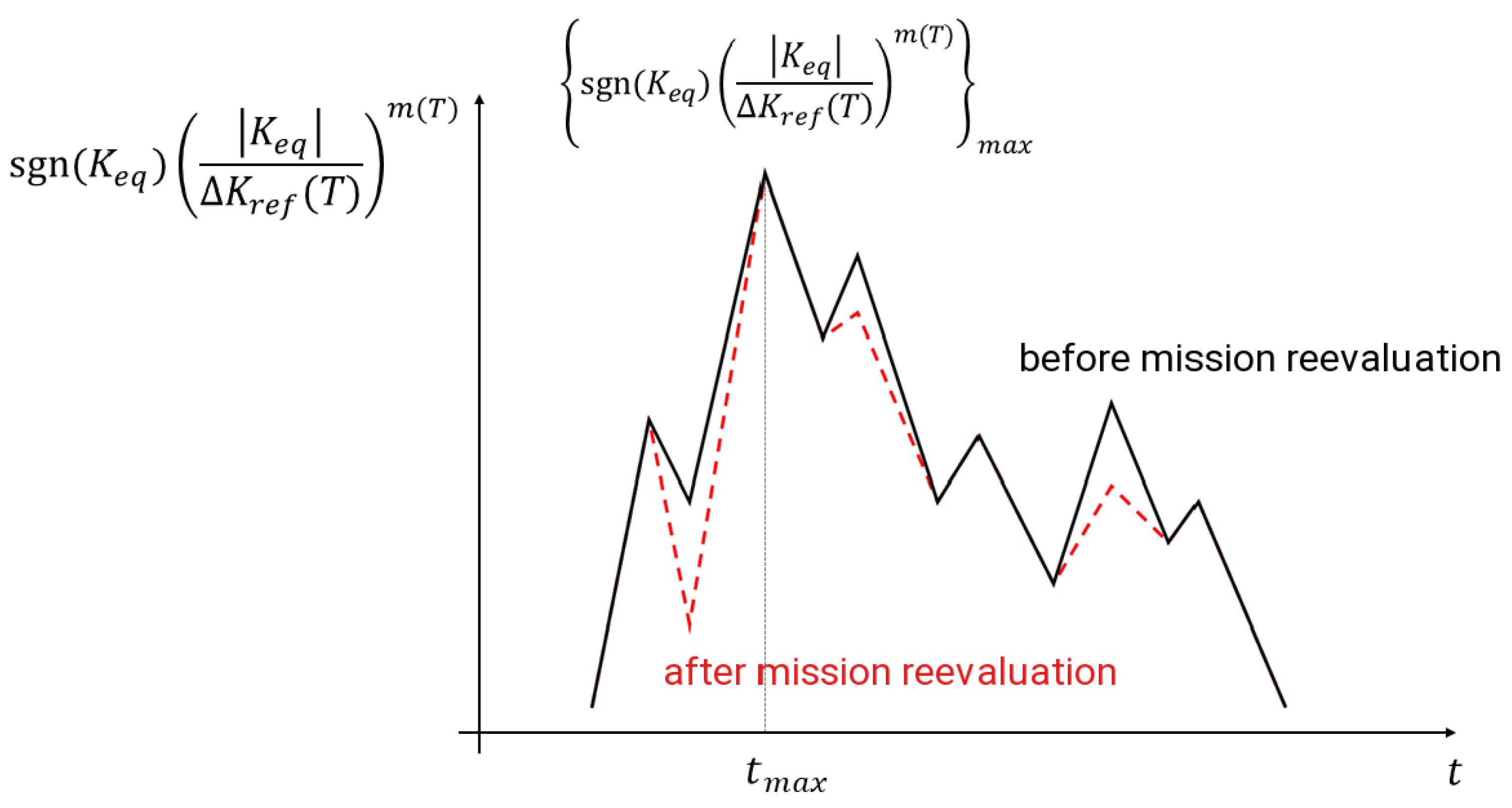
where m and $\mathsf{\Delta }{K}_{ref}$ are temperature-dependent material properties. Since for single loading steps, $K_{eq}$ may be negative (which happens in rare cases), the absolute value is taken under the exponentiation, and the sign is moved ahead of the brackets. Consequently, a fictitious negative $da/dN$ is assigned to a purely compressive load step. A hypothetical time distribution of the resulting values for $\frac{da}{dN}$ at a given crack front location is shown in Figure 8 (continuous black lines). Notice that this curve not only contains information on the loading, but also on the way the material reacts to this loading at the given temperature (through the Paris law). Subsequently, the dominant step is identified, defined as the step at which $\frac{da}{dN}$ based on Equation (5) is maximal (time $t_{max}$ in Figure 8). Now, the assumption is made that the crack propagation direction due to the mission corresponds to the deflection angle calculated based on the dominant step. Therefore, the step, which leads to the maximum crack propagation rate according to Equation (5), dictates the growth direction.

Once the crack propagation direction is determined, the next step consists of re-evaluating the crack growth rate contributions for each zero-max cycle. During a mission, the principal plane corresponding to the largest principal value of the self-similar stress at each loading point can largely deviate from the previously defined dominant direction, and therefore, its contribution to the crack growth rate may be incorrect. To avoid this issue, CRACKTRACER3D assumes that for all other mission instants, the crack propagates on the principal self-similar plane, which is as close as possible to the dominant direction [50], and it is the corresponding $K_{eq}$ that is used to calculate $da/dN$ through Equation (5) for the subsequent cycle extraction. This means that, except for the dominant loading step, $K_{eq}$ used for cycle extraction is not necessarily equal to the maximum principal self-similar stress; its value may be lower, generating a lower crack growth rate, as shown by the red dashed lines in Figure 8. For a concrete application of this procedure, the reader is referred to [2].

After mission reevaluation, cycle extraction is applied to the new crack propagation rate distribution (the red dashed line in Figure 8) with the rainflow counting algorithm described in [5]. The reasoning behind this is that cycle extraction should be performed on a quantity that is as close as possible to what the outcome of the process is: the crack propagation rate (due to the mission). Therefore, it is reasonable not to base the extraction on a stress intensity factor history, but rather the crack rate history, which includes the effect of the stress intensity factors on crack propagation through the temperature-dependent crack propagation parameters.

Each extracted cycle has a maximum and a minimum value of $K_{eq}$, leading to $\mathsf{\Delta }{K}_{eq}=K_{eq}^{max}-K_{eq}^{min}$. These two extremes are characterized by the temperatures $T_{K_{eq}^{max}}$ and $T_{K_{eq}^{min}}$, respectively. The propagation rate due to this cycle is now taken to be the maximum of $\frac{da}{dN}\left(T_{K_{eq}^{max}}\right)$ and $\frac{da}{dN}\left(T_{K_{eq}^{min}}\right)$, i.e., $da/dN$ for $\mathsf{\Delta }{K}_{eq}$ is once calculated at $T_{K_{eq}^{max}}$ and once at $T_{K_{eq}^{min}}$, and the maximum is taken. This approach allows remaining on the conservative side since there are some materials that show a decrease of the crack growth rate for increasing temperature in certain temperature ranges. In the end, the crack growth rate due to the mission is given by the sum of the crack growth rate for each extracted cycle.

The essence of the present method is the concept of a dominant loading step enforcing its crack propagation direction on the complete mission. Alternatively, one comes in the literature across concepts using the propagation direction of all loading steps in the mission [37]. The idea is to consider the deflection angle as a weighted average of the crack deflection angles of each step. One approach is to take the equivalent K-factors as weighting factors. However, here, the crack propagation rate in accordance to Equation (5) is proposed as the weighting factor, in agreement with the philosophy to use quantities related to the growth rate rather than the loading. Thus, the new deflection angle satisfies the following equation:

$$\phi =\frac{{\sum }_{i=1}^{Nstep}{\phi }_i{\left(\frac{da}{dN}\right)}_i}{{\sum }_{i=1}^{Nstep}{\left(\frac{da}{dN}\right)}_i}$$

(6)

where i is the i-th static step and $Nstep$ is the total number of static steps used to discretize the mission. This alternative approach to calculate the crack propagation direction will be compared with the dominant step approach in the following section.

5. Validation Using the Tension-Torsion Tests

Experimental and numerical results for the tension-torsion tests were compared to validate the accuracy of CRACKTRACER3D in predicting the crack propagation direction. To this end, the outside surface of the broken specimens was measured by a GOM ATOS machine using blue light scanning. The result was a very detailed triangulation of the fracture surface. This surface was compared with the triangulation of the propagated crack surface predicted by CRACKTRACER3D. In order to do that, a new software called CT3D_Validator [51] was developed at MTU Aero Engines AG. The basic concept is to find a parameter that measures the deviation between the numerical and experimental crack propagation directions. The two crack surfaces to compare are both meshed with triangles. The idea is to calculate the volume between these two triangulations and then divide it by the CRACKTRACER3D crack surface area. Thereby, the final result is a length called d that quantifies the global deviation between the two crack directions and satisfies:

$$d_{ax}=\frac{{\sum }_{i=1}^N{V}_i}{{\sum }_{i=1}^N{A}_i}=\frac{{\sum }_{i=1}^N{d}_i{A}_i}{{\sum }_{i=1}^N{A}_i}$$

(7)

where the subscript $ax$ indicates the direction along which d is measured. For this type of specimen, $ax$ represents the longitudinal axis (i.e., the tensile direction). The index i identifies the i-th element of the CRACKTRACER3D crack surface, and N is its total number of elements. The volume is approximated with a group of triangular prisms built taking as a reference the numerical triangulation. For each triangle, a prism is extruded along the axial direction as high as the distance $d_i$ between the center of gravity of the i-th reference triangle and the experimental surface. $A_i$ is the triangle area of the i-th element. A graphical representation can be observed in Figure 9.

The deviation $d_{ax}$ was calculated to compare the dominant step criterion (labeled “current”) with the averaged angle criterion (labeled “new”) for the tension-torsion test results. More specifically, the eighteen possible load combinations were simulated with the two different criteria and compared with the same experimental result. In

Table 4. Specimens load combinations and deviation results.

No.	Label	${\mathit{R}}_{\mathit{axial}}$	${\mathit{R}}_{\mathit{torsion}}$	Phase (°)	$\frac{{\mathit{\tau }}_{\mathit{N}}}{{\mathit{\sigma }}_{\mathit{N}}}$	${\mathit{d}}_{\mathit{ax}}$ (mm) (Current)	${\mathit{d}}_{\mathit{ax}}$ (mm) (New)	${\mathit{a}}_{\mathit{surf}}$ (mm)	${\mathit{d}}_{\mathit{ax}}$ (%) (Current)	${\mathit{d}}_{\mathit{ax}}$ (%) (New)
1	$0\_1\_00\_1$	0	−1	0	1.31	0.2881	0.3663	4.6695	6.17	7.84
2	$0\_1\_00\_2$	0	−1	0	1	0.3332	0.4129	5.0724	6.57	8.14
3	$0\_1\_00\_3$	0	−1	0	0.76	0.4120	0.4920	5.8457	7.05	8.42
4	$0\_1\_40\_1$	0	−1	40	1.31	0.3876	0.4979	3.9610	9.79	12.57
5	$0\_1\_40\_2$	0	−1	40	1	0.4894	0.6183	3.9556	12.37	15.63
6	$0\_1\_40\_3$	0	−1	40	0.76	0.5275	0.6212	3.0564	17.26	20.32
7	$0\_1\_90\_1$	0	−1	90	1.31	-	-	-	-	-
8	$0\_1\_90\_2$	0	−1	90	1	0.0827	0.0694	0.5843	14.15	11.87
9	$0\_1\_90\_3$	0	−1	90	0.76	0.0932	0.0908	0.7967	11.70	11.40
10	$1\_1\_00\_1$	−1	−1	0	1.31	0.0973	0.0971	4.9594	1.96	1.96
11	$1\_1\_00\_2$	−1	−1	0	1	0.2289	0.2307	5.0346	4.55	4.58
12	$1\_1\_00\_3$	−1	−1	0	0.76	0.0998	0.1010	5.8481	1.71	1.73
13	$1\_1\_40\_1$	−1	−1	40	1.31	0.3133	0.3460	3.9614	7.91	8.73
14	$1\_1\_40\_2$	−1	−1	40	1	0.1326	0.1732	3.9414	3.36	4.39
15	$1\_1\_40\_3$	−1	−1	40	0.76	0.0694	0.0577	3.8992	1.78	1.48
16	$1\_1\_90\_1$	−1	−1	90	1.31	-	-	-	-	-
17	$1\_1\_90\_2$	−1	−1	90	1	0.0600	0.0578	0.4978	12.06	11.60
18	$1\_1\_90\_3$	−1	−1	90	0.76	0.1545	0.1106	3.7642	4.11	2.94

, the first six columns show the load conditions, and in the next two columns, the results for $d_{ax}$ are summarized and compared for the two methods. Moreover, $d_{ax}$ was also calculated as a percentage of the crack propagation length $a_{surf}$ measured on the specimen free surface. In this way, it was possible to compare all eighteen cases. The main goal was to verify the crack propagation next to the notch tip, where it can easily be identified on the experimental surface. Therefore, for each specimen, CRACKTRACER3D stopped the propagation, trying to keep the crack progress within this region (before the final rupture). To achieve a proper comparison, the numerical analyses were run trying to keep the same $a_{surf}$ for both methods. For some load conditions, multiple test results were available. In such cases, the result with the clearest crack propagation surface was chosen for the comparison (the actual specimen number in that case is listed in

Table 5. Experimental deflection angle and numerical deviation (current).

No.	Label	Specimen Number	${\mathit{R}}_{\mathit{axial}}$	${\mathit{R}}_{\mathit{torsion}}$	Phase (°)	$\frac{{\mathit{\tau }}_{\mathit{N}}}{{\mathit{\sigma }}_{\mathit{N}}}$	$\mathit{\phi }\left({}^{°}\right)$	$\mathsf{\Delta }\mathit{\phi }\left({}^{°}\right)$
1	$0\_1\_00\_1$	61	0	−1	0	1.31	44.5	2.5
2	$0\_1\_00\_2$	63	0	−1	0	1	39.8	2.9
3	$0\_1\_00\_3$	62	0	−1	0	0.76	31.6	3.4
4	$0\_1\_40\_1$	85	0	−1	40	1.31	55.6	3.2
5	$0\_1\_40\_2$	73	0	−1	40	1	48.3	4.7
6	$0\_1\_40\_3$	75	0	−1	40	0.76	44.9	6.9
7	$0\_1\_90\_1$	-	0	−1	90	1.31	-	-
8	$0\_1\_90\_2$	65	0	−1	90	1	0.0	8.1
9	$0\_1\_90\_3$	60	0	−1	90	0.76	12.3	6.5
10	$1\_1\_00\_1$	87	−1	−1	0	1.31	41.2	0.8
11	$1\_1\_00\_2$	67	−1	−1	0	1	37.6	2.1
12	$1\_1\_00\_3$	81	−1	−1	0	0.76	23.3	0.9
13	$1\_1\_40\_1$	94	−1	−1	40	1.31	48.4	3.0
14	$1\_1\_40\_2$	71	−1	−1	40	1	34.7	1.6
15	$1\_1\_40\_3$	97	−1	−1	40	0.76	28.4	0.9
16	$1\_1\_90\_1$	-	−1	−1	90	1.31	-	-
17	$1\_1\_90\_2$	70	−1	−1	90	1	18.1	6.5
18	$1\_1\_90\_3$	83	−1	−1	90	0.76	0.0	2.4

.

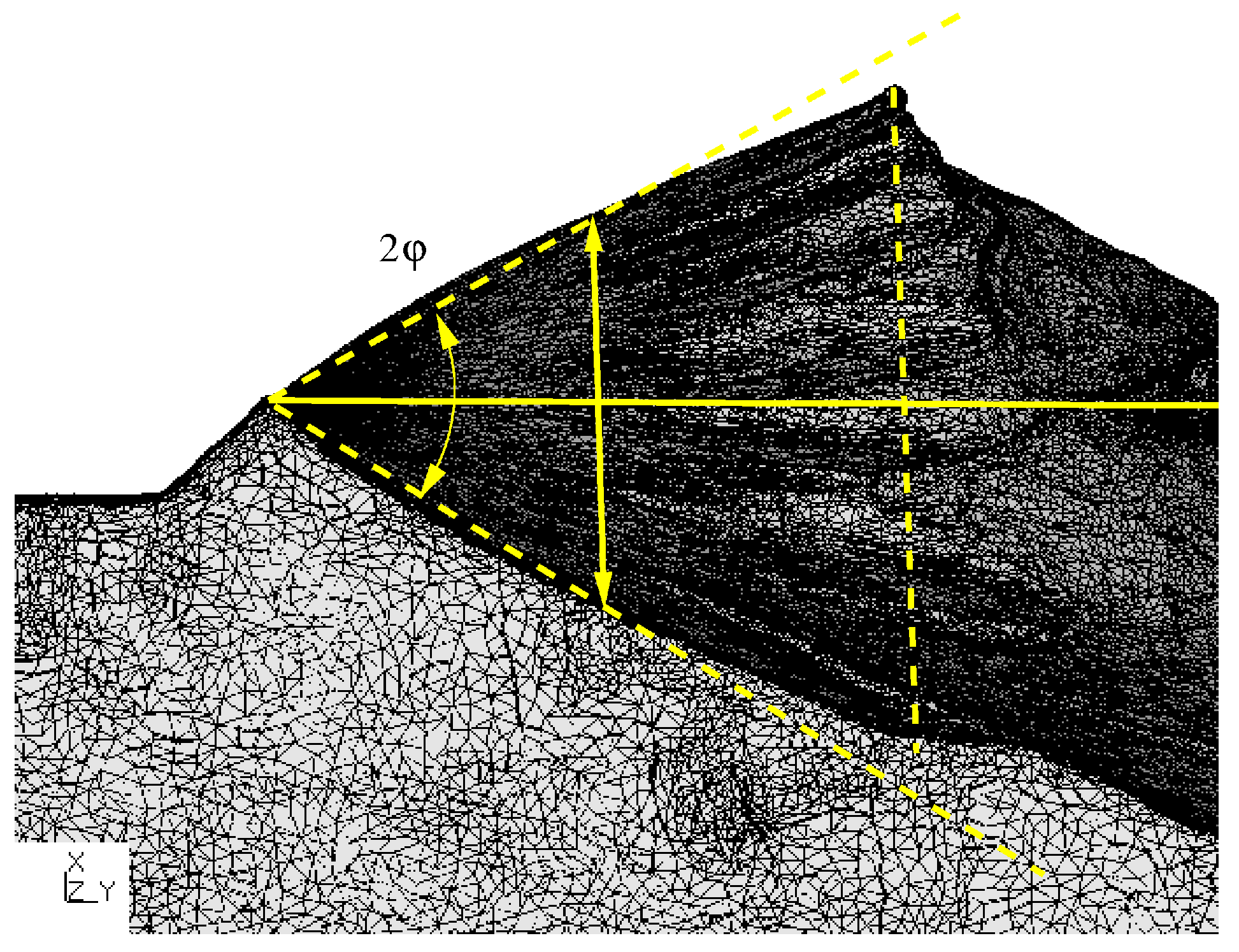
For the dominant step criterion, the relative deviation (second, but last column in Table 4) was converted into an approximate deflection angle by $\mathsf{\Delta }\phi ={tan}^{-1}(d_{ax}[\%]cos\left(\phi \right))$. It is listed in Table 5 together with an estimate of the absolute deflection angle $\phi$ based on the experimental results. This estimate was obtained by orienting the triangulation of the fractured specimens in the thickness direction (Figure 10). The torsion applied to the specimens led to a positive deflection angle on one face of the specimen and a negative one on the other face. By looking in the thickness direction, both are superimposed. Then, the propagation range of interest was identified (from the notch tip up to the dashed vertical line in the figure). At half this distance, the angle $2\phi$ was measured and divided by two. This procedure worked well except for the specimens with a 90° phase shift, as will be explained next.

Before looking at the comparison between the experiment and numerical prediction, it is worthwhile to have a more detailed look at the experimental results themselves in the form of the deflection angle. For pure tension, the deflection angle was zero; for pure torsion, one ends up with a deflection angle of $\pm 62°$, taking the K-values published in [38] and the deflection angle formula by Richard [3]. For the tension-torsion loading, the values should be somewhere in between. Looking at the column for $\phi$ in Table 5, one can conclude for phase shift 0° and 40° the following:

• For fixed $R_{axial}$ and a fixed phase shift, the deflection angle increases with increasing torque. This is to be expected since the torsion leads to the nonzero deflection.
• Changing $R_{axial}$ from zero to −1 leads to a decrease of the deflection angle. This also seems logical since the crack opening function by Newman [52] decreases for R decreasing from zero to −1. This means that for decreasing R in that range, the effective stress intensity range due to the tensile force increases, leading to less deflection. The increasing friction between the crack surfaces for $R=-1$ may also play a role.
• In nearly all cases, a switch from a 0° to a 40° phase shift leads to an increase of the deflection angle. This indicates that the time at maximum tensile force, which corresponds to a higher tension/torsion stress ratio compared to zero phase shift, is not dictating the crack propagation direction. To the contrary, the time at which the tensile to torsion stress has decreased must be dominant for a phase shift of 40°.

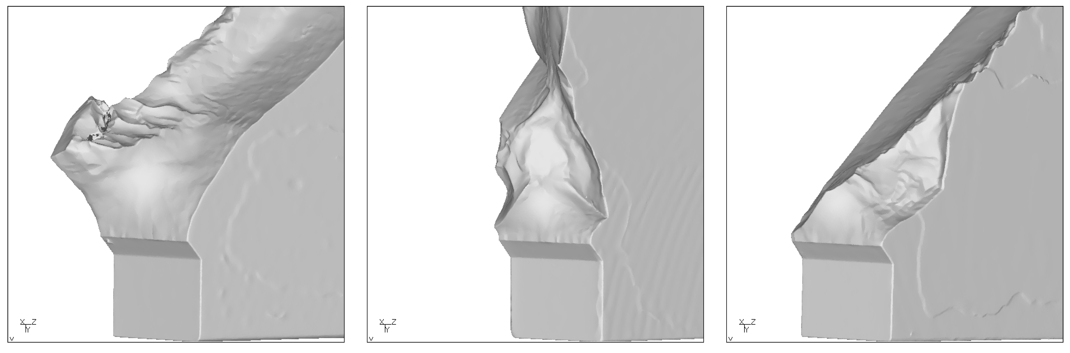
For a phase shift of 90°, the picture is much more difficult. For the specimens 0_1_90_1 and 1_1_90_1 ($\frac{{\tau }_N}{{\sigma }_N}$=1.31), the experimental results are not consistent. This is illustrated in Figure 11 and Figure 12. The figures show three different results for three different specimens with the same loading conditions. Therefore, a deflection angle could not be determined.

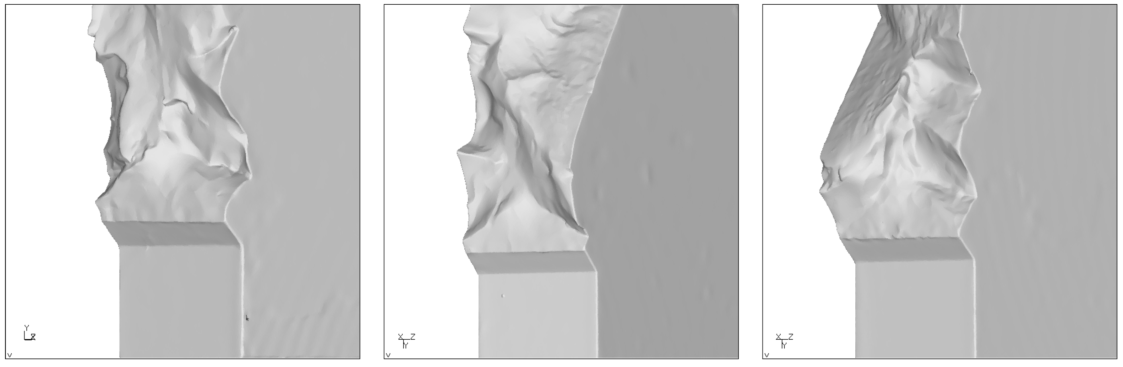
Specimens 0_1_90_2 and 1_1_90_2, for which $\frac{{\tau }_N}{{\sigma }_N}$ = 1, are shown in Figure 13. Specimen 0_1_90_2 in Figure 13a (the view angle for this specimen was chosen differently from the other specimens, in order to have a better view on the crack surface) shows propagation in the same direction at both free surfaces; only at crack front positions immediately underneath the right free surface, a local area with propagation in the opposite direction can be noticed. Specimen 1_1_90_2 (Figure 13b) shows a more or less flat crack surface across the complete thickness of the specimen. Only very near the free surface, some wavy deflection can be noticed. Therefore, determining a deflection angle is difficult and was only done for $R_{axial}$ = −1.

Finally, for specimens 0_1_90_3 and 1_1_90_3, for which $\frac{{\tau }_N}{{\sigma }_N}$=0.76, the crack surface was more or less flat, with some wavy behavior at the free surfaces. Here also, it was very difficult to measure any deflection angle. Summarizing, the results for a phase shift of 90° are ambiguous for a high torsion/tension ratio and tend to very low deflection angles the smaller this ratio is.

The last column in Table 5 shows the deviation of the deflection angle for the dominant step criterion. The following observations can be made:

• The deviation is generally quite low, which means that the underlying physical phenomena are well covered.
• The deviation increases for increasing phase shift. It is only for nonzero phase shift that steps in the mission really start to compete. Therefore, more deviation is expected.
• The deviation for $R_{axial}$ = −1 is less than for $R_{axial}$ = 0. In the latter case, the tensile loading is less dominant (higher value of the crack opening function, i.e., smaller effective $\mathsf{\Delta }K$ range; furthermore, there is less friction between the crack faces, leading to a higher effect of the torsional loading), leading to a higher competition between the loading steps.
• For the in-phase and 40° out-of-phase cases with axial traction ($R_{axial}=0$), it is evident that the higher the torsional moment, the more precise the numerical results are. When the axial force is applied with tension and compression ($R_{axial}=-1$), this is not so.

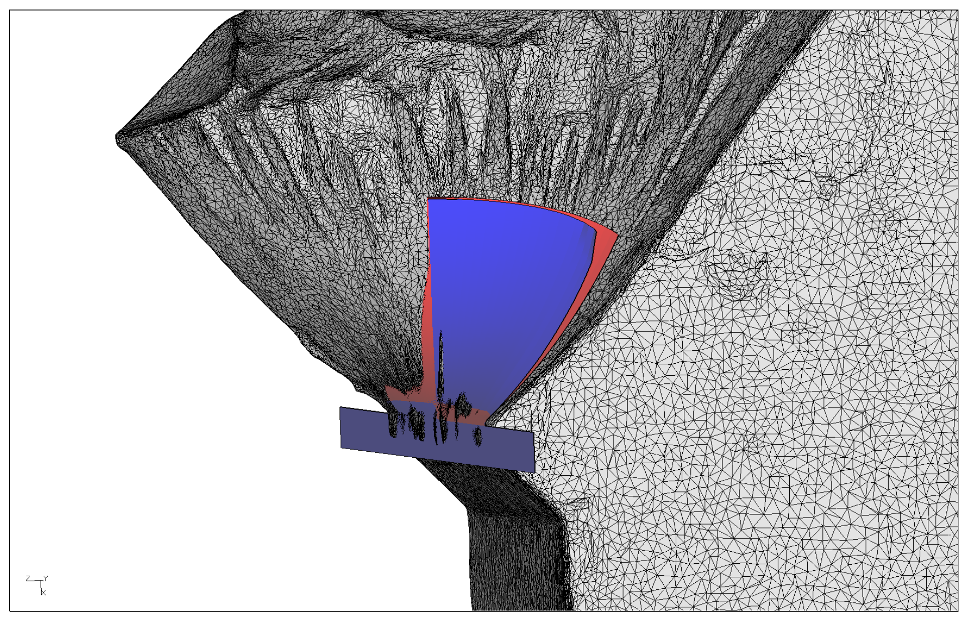
In order to judge the potential of the dominant step versus the averaged angle criterion, the last two columns in Table 4 should be looked at. In the case of $R_{axial}=0$ and a 0° phase shift, the current method generates a numerical prediction with a lower $d_{ax}$ (%) than the new one. Indeed, as shown in Figure 14, the crack surface computed with the current criterion (in red) evolves nearer to the experimental surface (black triangulation) than the numerical prediction by the new approach (in blue). In this and subsequent figures, the right half of the broken specimen is shown. In the lower part of the figure, one notices the V-shaped starter notch. The blue rectangle represents the initial crack introduced by Mode I controlled fatigue. The (red and blue) numerically calculated crack propagation surfaces are only visible if they lie in front of the experimental surface. Since both the numerical, as well as the experimental surfaces are antisymmetric across the thickness due to the torsional loading, this is the case for half of the crack front (in the actual case, for the half that is closest to the observer).

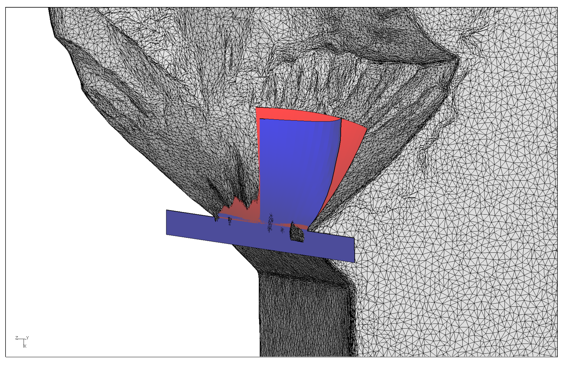
Analogously, the same findings can be observed for $R_{axial}=0$ and a 40° phase shift. Figure 15 provides the reader with a graphical representation of specimen 0_1_40_2. Although the numerical crack behavior replicates the real surface trend evolution, the deviations are higher than for the in-phase cases.

The difference between the dominant step and the averaged angle method becomes less significant for $R_{axial}$ equal to −1. For the specimen 1_1_00_1, $d_{ax}$ (%) rounded to the second decimal digit is totally the same, as also graphically visible in Figure 16, where the two methods have almost identical predictions. For a 0° and a 40° phase shift, the current method is slightly more precise.

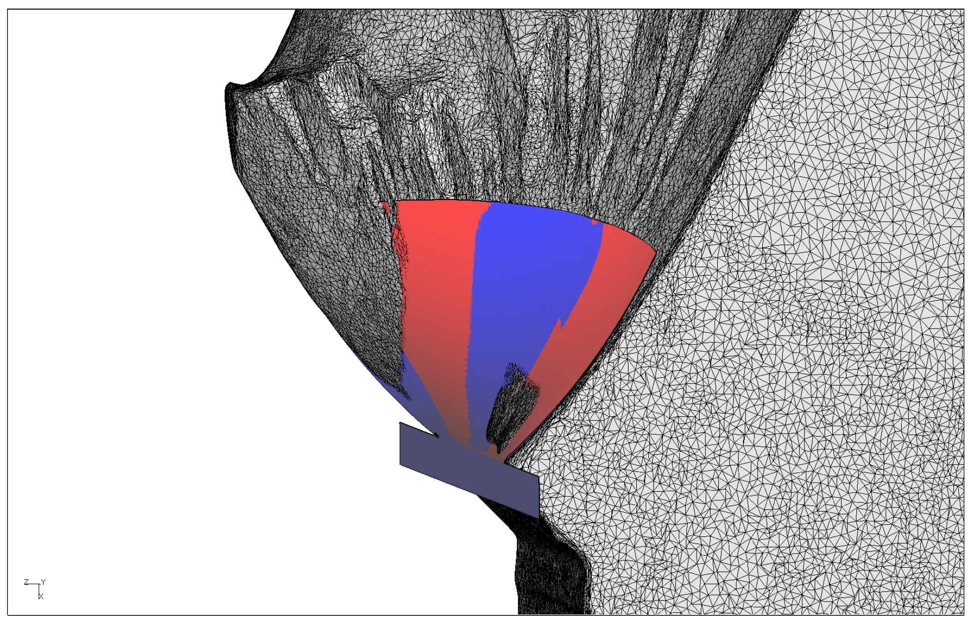
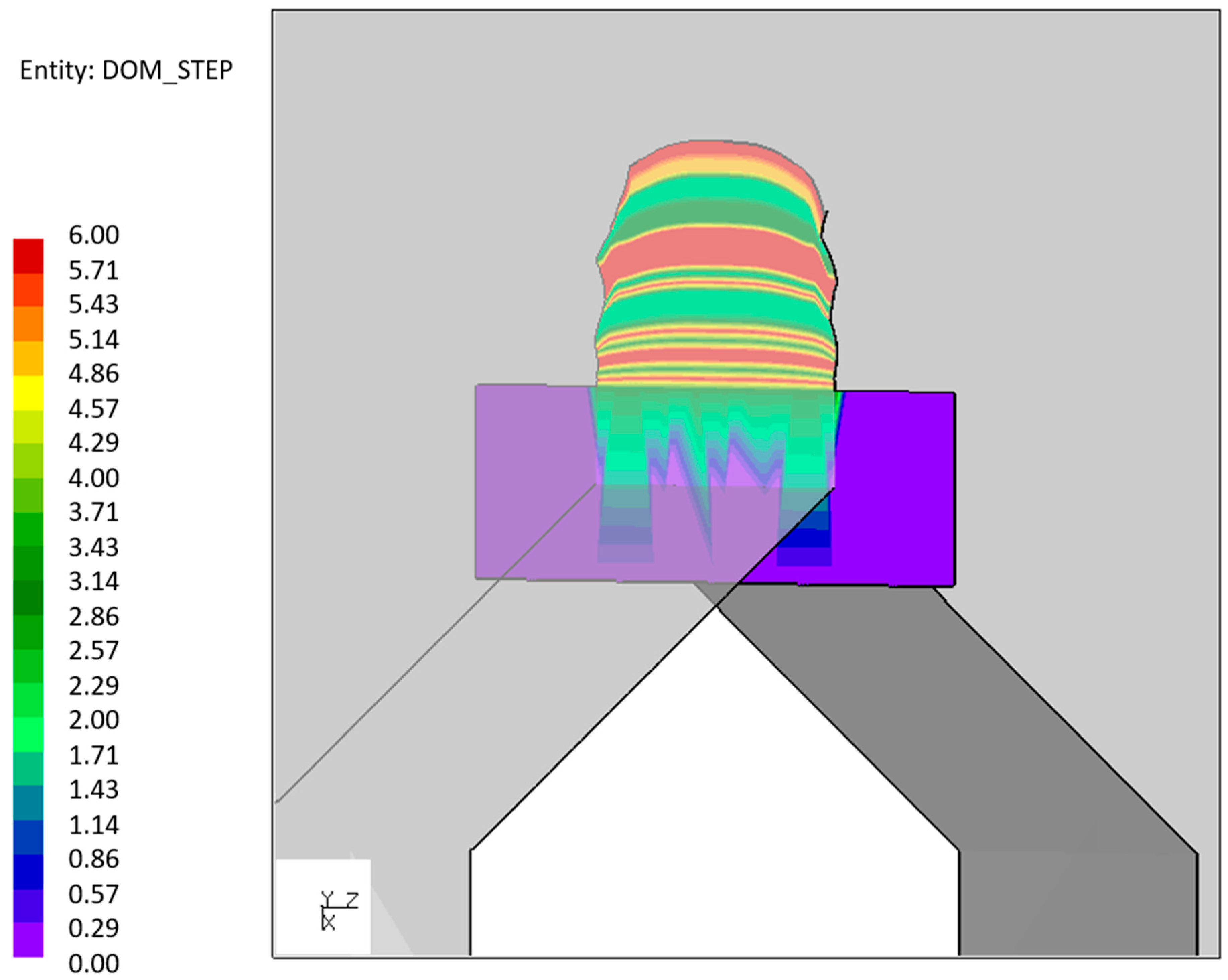
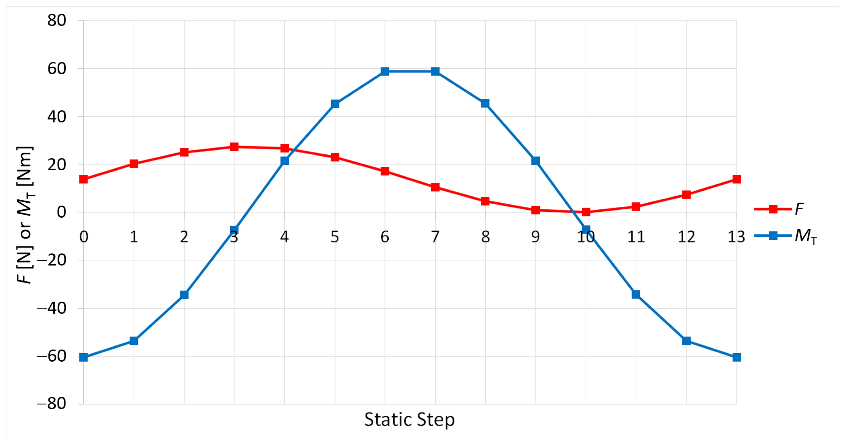
When the phase shift is equal to 90°, the current method leads to a wavy behavior of the crack propagation surface due to the dominant step identification procedure for the crack deflection angle. For instance, the dominant step on the crack surface for specimen 0_1_90_3 is shown in Figure 17, whereas Figure 18 shows its load sequence versus step number. The result in Figure 17 shows a continuous switch of the dominant step in the step range 2–6. These are the steps in the neighborhood of the maximum F and increasing $M_T$. This phenomenon does not occur with the new method because of an intrinsic smoothing due to the weighted average in the crack deflection angle definition. The values of $d_{ax}$ from Table 4 result in being more precise for the new method. Nevertheless, the experiments for a 90° phase shift showed large variability and a tendency to grow in-plane, which seem to match the idea of a steadily shifting dominant step.

6. Conclusions

Through experimental results, the CRACKTRACER3D numerical prediction is compared for crack propagation analyses in mixed-mode missions. To choose the crack propagation direction, a new approach based on an average deflection angle criterion is implemented in the post-processor. To identify the crack propagation accuracy of the numerical solution with respect to the experimental one, a measure based on the average distance between the experimental and numerical crack surface is defined. The results show a lower accuracy for virtually all 0° and 40° phase shift tests analyzed by the average angle implementation, proving the validity of using the dominant step to choose the crack propagation direction. The cases with 90° out-of-phase loads result in slightly lower deviations with the average angle criterion. However, since in these tests, some doubt arose about the reproducibility of the experimental crack surface, these findings have to be considered with care. Either way, the results encourage further experimental investigations with different loading missions.