Article

Jupyter Notebooks in Undergraduate Mobile Robotics Courses: Educational Tool and Case Study

by
Jose-Raul Ruiz-Sarmiento
*,
Samuel-Felipe Baltanas
and
Javier Gonzalez-Jimenez
Machine Perception and Intelligent Robotics Group (MAPIR), Department of System Engineering and Automation, Biomedical Research Institute of Malaga (IBIMA), University of Malaga, 29071 Málaga, Spain
*
Author to whom correspondence should be addressed.
Appl. Sci. 2021, 11(3), 917; https://doi.org/10.3390/app11030917
Submission received: 3 December 2020 / Revised: 12 January 2021 / Accepted: 15 January 2021 / Published: 20 January 2021
(This article belongs to the Special Issue Advances in Artificial Intelligence Learning Technologies)

Abstract

:

Featured Application

A novel tool to successfully bolster underpinning concepts and techniques in robotics courses in the context of STEM education.

Abstract

Jupyter notebooks are recently emerging as a valuable pedagogical resource in academy, being adopted in educational institutions worldwide. This is mainly due to their ability to combine the expressiveness of traditional explanations from textbooks, with the interaction capabilities of software applications, which provides numerous benefits for both students and lecturers of different fields. One of the areas that could benefit from their adoption is such of mobile robotics, whose recent popularity has resulted in an increasing demand of trained practitioners with a solid theoretical and practical background. Therefore, there is a need of high quality learning materials adapted to modern tools and methodologies. With that in mind, this work explores how the introduction of Jupyter notebooks in undergraduate mobile robotic courses contributes to improve both teaching and learning experiences. For that, we first present a series of (publicly available) educational notebooks encompassing a variety of topics relevant for robotics, with a particular emphasis in the study of mobile robots and commonly used sensors. Those documents have been built from the ground up to take advantage of the Jupyter Notebook framework, bridging the typical gap between theoretical frame and interactive code. We also present a case study describing the notebooks usage in undergraduate courses at University of Málaga, including a discussion on the promising results and findings obtained.

1. Introduction

Jupyter notebooks are documents combining in the same place narratives with texts, equations, figures, videos, links to additional resources, etc., as well as executable code with visible outputs [1]. Notebooks’ primitives are cells containing narratives formatted using different markup languages like HTML, Markdown, SVG, or LaTeX, or code written in a variate of languages such as Python, R, C++, Java, etc. [2]. As a result, they allow for the fast prototyping and development of contents of diverse nature [3] (see Figure 1). They are designed using the Jupyter Notebook application, a web-based development framework part of the Project Jupyter initiative [4]. The early popularity of this tool (back in 2014) was due to its virtues as an ecosystem for doing data science. However, nowadays it is standing out for the creation of teaching material, since it promotes the achievement of typical learning objectives posed by teaching plans worldwide (acquisition of basic knowledge, ability to evaluate and create, etc.) [3,5]. One of the main reasons for that is the ability of Jupyter notebooks for proposing challenging contextualized problems, where students have at their disposal the narratives and code needed for successfully address them. In this way, Jupyter notebooks are considered valuable resources for enhancing students engagement, participation, and understanding, which results in an increased performance and preparation for their carriers. They also provide instructors with mechanisms to gradually develop publishable and interactive material for lab assignments, in-class demos, auxiliary materials, etc. [3]. These documents are also called computational narratives or living documents, since students can interact with them to explore or focus on questions of interest for their learning, i.e., they can converse with a problem surrounded by relevant explanations, prose and code (experiments). From the educators side, Jupyter notebooks permit them to bring concepts to live during lectures.
One of the fields that can greatly benefit from the inclusion of Jupyter notebooks is such of the teaching of mobile robotics. Specifically, mobile robots are increasingly landing in fields like education, health care, surveillance, etc. [6,7,8], and might be as diverse as drones, autonomous cars, or warehouse robots, among others [9,10]. Nowadays, it is clear the commitment of public entities for advancing in this respect, as shown by the European Union through the H2020 Research and Innovation programme [11], United States or Japan [12]. Large, international companies like Google or Facebook are also aware of the possibilities of robots, showing a clear interest in mobile robotics-related companies and applications. As a consequence of this interest, the number of professionals and enthusiasts in the mobile robotics field is growing considerably, which demand a quality training in robotics-related topics. Indeed, the number of courses addressing such topics is also growing in universities as well as in online learning platforms like Coursera (https://www.coursera.org/) or Udacity (https://www.udacity.com/).
Mobile robotics courses integrate abstract concepts from diverse areas like algebra, probability, statistics, calculus, discrete mathematics, programming, or artificial intelligence [13], all of them present in STEM education programs [14,15]. The acquisition and understanding of such concepts by the students is essential to appropriately address varied topics in this field, including: robot motion, perception, localization, environment mapping, motion planning, and robotic control architectures among others [13,16,17]. The utilization of techniques from the artificial intelligence field is also ubiquitously present in most of those topics, e.g., they permit a robot to build a map of its workspace, localize itself within it, or even navigate through it, infer high-level information from sensory data, etc. In this way, to achieve such a quality training, they are needed both: to obtain a solid background about the theory behind these topics, as well as to put them into practice. Hands-on exercises are usually structured as lists of issues to be faced by the student, also relying on auxiliary or skeleton code if needed. Although it is a perfectly reasonable methodology in some fields, it might hampers the connection between complex theoretical concepts and practical assignments. This is the point where Jupyter notebooks can show their potential, since they pose the exploration and strengthening of theoretical concepts in an interactive and contextualized environment. However, educators entering the Jupyter Notebook ecosystem might get lost in the enormous amount of available resources (tutorials, blog posts, videos of talks, etc.) when looking for the best adoption practices. A simple search for the words “Jupyter Notebook tutorials” in Google returns 1,700,000 results.
In this work we explore the utilization of the Jupyter Notebook technology in undergraduate mobile robotics courses to enhance the experience of both students and lecturers. Its contribution is twofold. First, it describes a collection of Jupyter notebooks that have been devised to cope with the aforementioned issues, which coherently interweave narratives and interactive programming for contextually posing problems. Then, we present a case study addressing its usage by students and lecturers at an undergraduate course from the Computer Science degree at the University of Málaga (Spain), discussing the obtained results and findings as rigorously as possible.
The provided notebooks serve as an introductory resource for the field of mobile robotics, since they cover its typical topics: probability fundamentals, robot motion, sensor modeling, localization, map building, etc., [13,17]. Thereby, they can be directly adopted by educators, or edited to suit particular needs. By applying them to academia we obtain a tool to incrementally build reproducible exercises targeted at student consumption, i.e., being first and foremost accessible and easy to understand by them using rich text components, figures, code cells, etc. [4]. Each notebook comprises a number of related tasks that are put into theoretical context through computational narratives, yielding invaluable aid to the student in order to comprehend the underlying theory. Regarding the coding part of the exercises, the developed notebooks rely on the trending, general purpose programming language Python [18], given its seamless integration with Jupyter Notebook. Similarly to other pedagogical resources, we maintain two versions of the notebooks: the student version, which proposes a number of tasks for the student to complete, and the lecturer version that also includes their solutions. The former has been made publicly available at: https://github.com/jotaraul/jupyter-notebooks-for-robotics-courses, while the latter can be individually requested by any lecturer.
The remaining of this paper is as follows. Section 2 sets the theoretical framework of the paper. Next, Section 3 defines the purpose of the research as well as the research questions. Then, the methods followed in the work are described (see Section 4), including the participants, lecturers, and subjects in the spotlight, the contributed educational tool, and the data sources for measuring its impact. Then, Section 5 presents and discusses on the obtained results, while Section 6 draws conclusions from the work done.

2. Theoretical Background

For the purpose of defining the goals of a learning experience, the Bloom’s taxonomy [19] is one of the most referenced and applied resources in education [20]. Said taxonomy can be interpreted as a staircase where each step represents a certain cognitive level of thinking, subsuming each step the previous one [5]. Such (revised) steps are: remember, understand, apply, analyze, evaluate, and create. This way, they range from the elementary acquisition and recall of basic facts and concepts, to the more complex justification of positions and decisions or the production of new, original work. As a staircase, it requires the achievement of the prior skill or ability (step) before accomplishing the next one [21]. With these components, the taxonomy endows lecturers with a grounded framework for defining learning goals and the pathway to achieve them [22]. The design model of learning by problem solving is widely followed within this framework and considered the most effective one to take students to the top of the staircase [23,24]. Jupyter notebooks are a suitable tool to implement such paradigm, since they permit students to explore, analyze, synthesize and evaluate the teaching material in order to reach the pursued level of understanding [3,25]. Moreover, they also support the achievement of said goal promoting collaboration between students [4,26].
The aforementioned learning by problem solving design model is naturally aligned with others like project-based learning [27], inquiry-based learning [28], cooperative learning [29], or apprenticeship [30], to name a few, all of them under the umbrella of experiential learning [31,32]. Perhaps one of the most popular theorists in experiential learning is such of John Dewey, the precursor of the learning by doing concept [33,34]. These learning models are tightly related to constructivism in education: “an approach to learning that holds that people actively construct or make their own knowledge and that reality is determined by the experiences of the learner” [35,36], that is, learning is a result of an experiential process. Within that process—as promulgated by the Dale’s learning cone [37,38]—, it is well-established that students retain more information from direct, powerful experiences (what they do) than from what they see (videos, presentations), hear or read. Jupyter notebooks are well suited for designing such experiences, given their potential to create immersive material that place students in the context of a situation where their acquired knowledge can be enhanced and leveraged to solve significant problems [26,39].
Jupyter notebooks can be also considered as valuable software scaffolds, that is, software features that allow students to complete complex tasks being novice in them [40]. This is crucial for climbing steps in our learning staircase while starting from the basics facts and concepts. Indeed, they can naturally implement narratives presenting concepts, putting them into the problem context, challenging the student with incomplete code facing it, and motivating he/she to reason about results and draw conclusions [3,26,41]. This also slots with worked examples: “a step-by-step demonstration of how to perform a task or how to solve a problem” [42]. It has been shown that when dealing with complex concepts that can be difficult to understand, worked examples with high level of guidance can enhance learning to a greater extent than those with lower levels of guidance [43]. This is a consequence of effectively structured worked examples producing affordable cognitive loads to students, which is also known as the worked-example effect [44].
Jupyter Notebooks can be also successfully applied to training programs based on STEM education [14,15]. STEM is the abbreviation of Science, Technology, Engineering and Mathematics, while STEM education stands for the joint learning of those disciplines instead of addressing them in isolation, resulting in an enhance of systematic thinking and problem-solving abilities [45,46]. It follows an Engineering approach, developing theoretical concepts for their posterior practical application [15,47]. Thereby, STEM proposes the joint learning of concepts from those topics within a hands-on process of design and problem resolution, emulating how Engineering performs in the real world. Specifically, the field of mobile robotics demands the learning of concepts from areas like algebra, probability, statistics, calculus, discrete mathematics, programming, or artificial intelligence, which are common and inherent to the aforementioned disciplines [13,48]. Computational narratives put those concepts in their proper context and encourage students to solve problems, typically inspired in the real world, which aligns perfectly with the purposes of STEM [49,50].
In summary, the Jupyter Notebook technology is emerging as a framework for the development of valuable teaching material for successfully reaching teaching goals in a menagerie of educational paradigms. Its application has been explored in some fields [3]. For example, the authors in [39] designed computational notebooks to teach Artificial Intelligence (AI), presenting them as offering a new mode of teaching and learning for the AI classroom. In [41], it is proposed the utilization of the Jupyter Notebook technology for setting an interactive learning environment for the introduction to process model discovery in the context of a course entitled “Process mining”. Regarding prerequisites of STEM subjects, the problem arising from the different levels of knowledge that students can exhibit is tackled in [49] by using Jupyter notebooks. Concretely, Jupyter Notebook was used to create an interactive, self-study course addressing Linear Algebra as a prerequisite for a Machine Learning course. The authors in [51] also resorted to this technology to develop dozens of Jupyter notebooks for training in seismology. In the field of mobile robotics, there are notebooks dealing with the Robot Operating System [52] (e.g., [53]), as well as works discussing the utilization of pedagogical tools, like code snippets in Matlab, in the scope of the traditional problem-solving approach [17,54]. However, to the best of our knowledge, this is the first work motivating and describing novel teaching material designed in the Jupyter Notebook framework and covering the fundamentals of mobile robotics, as well as a case study illustrating its application in academia.

3. Purpose of the Research

Mobile robotics courses encompass a wide range of complex and abstract concepts from different disciplines, which may hamper the learning process. This paper relies on experiential learning to orchestrate such process in undergraduate courses. Specifically, it studies how the pose of contextualized problems to be solved by the completion of worked examples may impact students’ performance. For that, it has been devised a novel educational tool consisting of a collection of Jupyter notebooks. Said notebooks aim to empower the students’ climbing of the steps in the Bloom’s taxonomy towards the achievement of the pursued learning goals. In mobile robotics courses, such goals are the understanding, design, and development/implementation of basic robotics skills such as robot motion, sensing, map building, localization, path planning, etc. Concretely, the learning programme of the courses in the spotlight (see Section 4.1) is targeted at the acquisition of the following knowledge/abilities by students:
  • To know and explain which are the fundamental problems so a robot can be considered autonomous.
  • To know the components of a robot (sensors, actuators, software, mechanical components, etc.) and how they operate in isolation and as components of a system.
  • To understand how the most used sensors for gathering information from the environment work, as well as their associated probabilistic models.
  • To comprehend the localization and map building process for a mobile robot.
  • To understand and develop motion planning algorithms.
  • To program a mobile robot so it navigates a 2D environment.
Thereby, the specific research questions addressed in this work are:
RQ1. 
Do Jupyter notebooks enhance learning in mobile robotics undergraduate courses?
RQ2. 
Do they represent an improvement over the traditional problem posing approach?
RQ3. 
Are they a suitable framework for designing hands-on sessions from the lecturers point of view?

4. Methods

4.1. Procedure

This study was carried out in the scope of the innovative education project Development of Interactive Documents to Empower Learning in Robotics-related Subjects. It comprises three consecutive academic courses of the Robotics subject (from 2017/2018 to 2019/2020), mainly devoted to mobile robots and common sensors in the field (e.g., odometers, cameras, laser scanners, sonars, etc.). This is a compulsory subject taught in the last of the four academic years of the Computer Engineering degree of the University of Málaga. It corresponds to six European Credit Transfer System (ETCS) [55], that is, to 150 h of student work. It spans over 15 weeks from October to January, where students attend to theoretical and practical lessons, and carry out two exams. Table 1 illustrates the course syllabus, which was the same during the three courses conforming this study (besides the number of sessions, which suffered minor changes). It is divided into 4 blocks entitled: Introduction to robotics, Mobile Robots, Mobile robot localization, and Motion planning. Regarding the courses’ teachers, the lecturer in charge of the theory lessons was the same in all of them, while for the practical lessons they were two: one for the 2017/2018 academic course, and another lecturer for 2018/2019 and 2019/2020 ones. However, 2017/2018 and 2018/2019 courses shared hands-on material and grading strategy.
During the last two academic courses, a Jupyter Notebook based approach has been developed to replace the traditional problem-solving one (see Section 4.2), which was finally introduced in the last course (2019/2020). As shown in Table 1, each theory topic is followed by a lab session to consolidate concepts and put them into practice (both theory and lab sessions last 2 h). In those hands-on sessions, students are given a Jupyter notebook. Such notebook is first introduced by the lecturer to explain its parts, which follow a worked example philosophy. Then, students start working on it while the lecturer is available to answer questions. Given that it is only needed a web browser to work with notebooks, they could work with the computers available in the classroom or bring their own laptops. A deadline was set (typically one week after the lab) for the students to submit a report including the completed notebook as well as a (guided) discussion about the work done and interesting findings. This submission was graded by the lecturers, which also provided feedback about possible issues/strengths. The grading scheme gave marks according to: (a) correctness of the solution, (b) elegance and originality of the solution, (c) correctness of the discussion, and (d) additional code/discussion cells added by the own student.
The traditional problem-solving approach replaced by the Jupyter Notebook based one relied on code snippets in Matlab along with problem definitions [54]. Concretely, students in the courses 2017/2018 and 2018/2019 faced hands-on sessions with skeletons of code addressing the same typical robotic problems as those included in the notebooks. Such skeletons exhibited parts where the code was removed, containing relevant concepts which understanding by the students was especially important in the course. However, we found that this approach has difficulties when contextualizing said code snippets and providing a comprehensive view of the addressed problems, being these the strengths of Jupyter notebooks. The reports’ submission and grading scheme were the same as previously described for the 2019/2020 course.
The study involved a total of 55 students, divided into 49 males and 6 females (a common ratio in STEM undergraduate subjects [56]). As Robotics is a subject in the last year of the degree, students have background knowledge about calculus, algebra, statistics, programming, etc., that is, in STEM related subjects. In this way, the subject offers an opportunity to combine previous concepts and tools from different STEM areas with new ones, and apply them to solve contextualized problems. This allows students to consolidate such background knowledge by using it in practice. Students’ previous knowledge and skills remain the same during the three academic courses in the scope of this work.

4.2. Educational Tool

One of the major contributions of this work is a novel educational tool, consisting of a collection of Jupyter notebooks addressing mobile robotics fundamental problems. Such notebooks permit students to face them and improve their skills by consolidating their knowledge, enhancing their understanding, implementing algorithms and reasoning and commenting on the obtained results. Next sections describe the technologies that we have resorted to in their development (see Section 4.2.1), as well as the notebooks themselves (Section 4.2.2).

4.2.1. Used Technologies

Jupyter Notebook

Jupyter Notebook [1] provides a platform to easily blend rich text elements and executable code in the same document. It is the work of Project Jupyter, an award winning [57] non-profit project, dedicated to the creation of open-source tools for interactive data science and scientific computing. The Jupyter Notebook framework is one of its most popular developments, and it is composed of a series of tools:
  • Notebook format. It organizes the code in a number of cells, which can be modified and run on demand. The outputs generated by these executions are displayed just beneath the code cell. Not only they can display text, but plots, graphics or mathematical formulas. Besides the code cells, there are text cells written using Markdown markup language (more information on that below).
  • Web application. It works as both a text and code editor and a computing platform. Its web application nature allows a lecturer to set up a server in order to give ready access to the platform if needed, although it can be easily installed in a local machine, e.g., using Anaconda (https://www.anaconda.com/distribution/).
  • Kernel. Language backend designed to execute code on request, using a common documented protocol. Initially, only a kernel for the Python programming language was available, yet the incredible popularity of the platform and its open-source nature has encouraged the development of an increasingly amount of kernels, now embracing over 50 additional languages (https://github.com/jupyter/jupyter/wiki/Jupyter-kernels).
Regarding the text cells provided by the notebook format, its support for Markdown (https://www.markdownguide.org/getting-started) provides powerful formatting options. It allows the inclusion of rich elements, such as mathematical formulas, tables, lists, images, links, static code, etc. Another benefit in comparison to other markup languages such as Applsci 11 00917 i001 or HTML, is Markdown’s rather minimal syntax, which allows newcomers to readily work without experiencing a heavy learning curve. Nonetheless, if a greater amount of control over the content of the document was needed, HTML can be also used within a text cell. This could be a really powerful tool, as most of the capabilities of HTML translate directly to the Jupyter Notebooks, such as embedding a video within them. Next section describes the programming language used in the code cells.

Python

The programming language of choice for the elaboration of the practical assignments is Python, one of the most popular languages nowadays, ranking just bellow C and Java [58]. Some of the reasons for such a popularity are its clean and concise syntax and a breadth of libraries for most use cases. This makes the language a great tool for prototyping and experimenting without the boilerplate coding conventions or significant compile time of other, more efficient, programming languages. Concretely, the practical exercises make use of the following libraries:
Numpy. 
The de facto library for matrix and array computation in Python. It provides a large collection of high-level mathematical functions, such as matrix multiplication, trigonometric functions, etc.
Scipy. 
A library for mathematical computation, which was originally Numpy’s parent project. It brings additional utilities for statistics, linear algebra and signal processing which are basic building blocks in the developed notebooks.
Matplotlib. 
Visualizing the problem pays a huge part in the learning process, specially in the domain of mobile robots. Matplotlib is a 2D plotting library that permits us to create different data visualizations along our exercises. It has native support in Jupyter notebooks, displaying and updating the figures inline.
In the context of robotics courses, we must also remark that Python is one of the two supported languages of the Robot Operating System [52], also known as ROS. ROS is a widely used robotic architecture, and provides utilities and libraries necessary to create modular robot applications. In this way, the student can gain insight into a general purpose programming language that can be used within a robotics-specific framework.

4.2.2. The Collection of Jupyter Notebooks

This section describes the contributed collection of Jupyter notebooks for mobile robotics courses, covering labs 1 to 7, and categorized according to their tackled topic. Most of the notebooks follow a common structure:
  • Introduction. Description of the topic to be addressed in the notebook, including relevant theoretical concepts introduced as text, figures, equations, etc. This section also put the notebook in the context of a real problem (e.g., robot localization in a shopping mall).
  • Imports. Code cell importing all the external modules needed to complete the assignment.
  • Utils(optional). Depending on the complexity of the exercise, some code can be provided to the student to assist the implementation.
  • Issues. Each exercise will be comprised of a number of issues or points to be solved, each one made up of some text cell describing it and some incomplete code cells.
  • Demos. In order to test the correctness of the assignment and illustrate the concepts of the exercise, there will be mostly complete code cells to create visualizations.
This structure implements the worked example approach [3,42,43,44], so inexpert students can end up developing an algorithm for, for example, localizing the robot within a map of its workspace. Next sections describe these notebooks and the topics they address with more detail. Notice that they are referenced as Lab. X, being X the session index as provided in Table 1.
It is also worth mentioning the content of the GitHub repository containing the notebooks’ collection. It is organized as follows:
  • images: directory containing the figures used in the notebooks’ narratives (see Figure 1 for an example).
  • utils: directory grouping together a number of utilities (Python .py files) that ease students’ implementations if needed, so they can focus on more relevant parts of the algorithms addressed in the notebooks (recall the third point in the previous list). Examples of these utilities could be a function for drawing a triangle representing a robot at a certain position and with a given orientation, a method for plotting the uncertainty about robot/landmarks localization by means of ellipses, a method for composing poses, another one building complex Jacobian matrices, etc.
  • .ipynb files: the Jupyter notebooks themselves.
  • LICENSE: a file describing the notebooks’ public license (GNU General Public License v3.0).
  • README: a file briefly describing the notebooks and their high-level dependencies.
  • requirements: a text file containing the packages on which the designed notebooks depend. It can be used to automatically install such dependencies by means of pip or Anaconda.

Lab. 1: Probability Fundamentals

Problem description. A solid, base knowledge of statistics is a must in courses dealing with mobile robots, sensors, and their inherent uncertainty [59,60]. In contrast to most industrial robots, which usually operates in controlled environments and do repetitive works (e.g., an assembly line), a mobile robot faces a wider range of workspace configurations and situations that lead to uncertainty in both the robot and world state. Mobile robots operate in environments where not everything is known a priori, making intelligent decisions based on sensory data. Among the most common sources of uncertainty we can find: dynamic environments, sensor disturbances, or unreliable movement systems. Thus, the field of mobile robotics found in the utilization of probabilistic approaches a principled way to handle this uncertainty, which have had great success as of late [13,61]. Such approaches are used to manage probabilistic models of the robot localization, the maps of its environment, the uncertainty in sensors’ observations and actuators’ actions, etc [17]. The core principle of this probabilistic robotics is to explicitly represent the uncertainty in the form of probability distributions, so it is needed some notions of probability to understand upcoming methods based on them.
Proposed notebook. The first series of notebooks focuses on this topic, with an special interest in the Gaussian distribution, given its ubiquitous use throughout the rest of the course. To reinforce the concepts there are three notebooks for practicing this topic, which are also meant to introduce the labs’ workflow:
  • Gaussian distribution. This notebook introduces the student to some basic concepts of interest, for instance: how a Gaussian distribution is defined and the generation of random samples from it (see Figure 2).
  • Properties. It serves to illustrate different properties and operations of Gaussians like the central limit theorem, sum, product, linear transformation, etc., letting the student to experiment with different distributions.
  • Multidimensional Distributions. It mirrors similar issues from the previous two parts, using multidimensional distributions instead.
In some cases, it is useful to visualize how the Gaussian changes with respect to some of its parameters. For this endeavor Jupyter notebooks provide ways to interact with the cells, such as the slider in Figure 2. This kind of widget will refresh the figure on change, passing its value to the underlying function. In addition to sliders, there are a wide array of widgets, most of them mirroring tools also available in HTML like buttons, selectors or text inputs. All of them are integrated into the Python environment and can be used to create more dynamic demonstrations.

Lab. 2: Robot Motion

Problem description. A fundamental aspect of robotics is the locomotion of wheeled robots [62]. This is not a trivial matter, since most wheeled robot kinematics have non-holonomic constraints, that is, they can not freely move in the space. In contrast to holonomic systems, which have absolute degree of freedom, non-holonomic wheeled robots move in circular trajectories. Most robots exhibit a differential drive motion system, characterized by having two independent wheels, one per actuator, although more complex configurations like those of cars of bicycles can be also modeled by the Ackermann steering motion system. These systems are of interest to understand how the position of the robot is affected by sending velocity commands to its motion controller. Compositions of robot poses can be used to track the global robot position after each of these motions.
The robot motion can be affected by errors due to wheel slippage, inaccurate calibration, limited resolution during integration (time increments), measurement resolution, unequal floor, etc [62]. These errors result in a final robot position that can differ from the expected one as set by the provided motion commands. To handle this there are probabilistic motion models that characterize the robot motion in probabilistic terms, being the most popular:
  • Velocity-based. Motion model where the robot is controlled using a pair v , w of linear and angular velocities, respectively, during a certain amount of time.
  • Odometry-based. This model abstracts the complexity of the robot kinematics, being most useful when wheel encoders are present, although other sensors like laser scanners can be used to compute the required pose increments [63]. In this case, the motion commands are expressed as an increment of the pose: [ Δ x , Δ y , Δ θ ] .
Using any of these two models, the result of executing a motion command is a probability distribution (a Gaussian one) modeling the new robot pose.
Proposed notebook. The goal of this series of notebooks is to familiarize the student with different aspects of robot motion and control commands, concretely:
  • Composition of noisy poses. The first assignment is to implement robot movement using pose composition and Gaussian noise, then generating a number of movement commands to traverse a square route, something which will become a familiar routine in the following tasks.
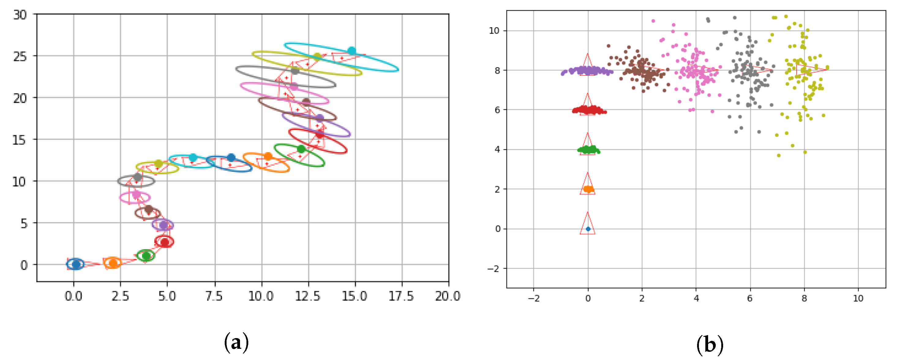
  • Differential motion with velocity commands. The following notebook introduces the equations for the differential motion model. Then asks the student to use velocity commands to move the robot in a serpentine trajectory as seen in Figure 3a.
  • Differential drive with odometry commands. Lastly, in order to reinforce the concepts of odometry commands the students apply them in both the analytical form ( x ¯ t , Σ x t ), and the sample form. The latter one is of special interest because of its utilization in particle filters [59]. It also better represents the real movement of a robot base (see Figure 3b).

Lab. 3: Robot Sensing

Problem description. The gathering of information from the environment, along with the movement models explained in the previous notebooks, comprise the essential basis for mobile robots (recall Mobile robots block in the course syllabus, Table 1). It is an incredibly broad topic, given the variety of sensors there exist, which can be roughly grouped into:
  • Proprioceptive sensors: those measuring the internal status of the robot: battery, position, acceleration, inclination. Some examples are: optical encoders, heading sensors (compass, gyroscopes), accelerometers, Intertial Measurement Units (IMUs), potentiometers, etc.
  • Exteroceptive sensors: sensors gathering information from the environment, like distance and/or angle to objects, light intensity reflected by the environment, etc. Examples of these kind of sensors could be range sensors (sonar, laser scanner [64], infrared, etc.) or vision based (cameras or RGB-D cameras [65]).
Real sensors do not deliver the exact truth of the quantities they are measuring, but a perturbed version. Thus, their operation is modeled through a probabilistic sensor model defining the function p ( z | v ) , where z is the variable representing the measurement and v the ground truth. For example, when dealing with a laser scan measuring distances, such a model is defined as p ( z | x , m ) , being x the sensor pose in the map m of the environment. To illustrate the basic concepts of this topic, we mainly focus on landmark observation models dealing with range-bearing sensors (e.g., stereo cameras, features in a scan, etc.). Such models consider that the map of the environment is a collection of landmarks m = { m i } , i = 1 , , N , hence simplifying problems like data association.
Proposed notebook. Students are challenged to implement a simulation of a range-bearing sensor and manipulate the information in a number of instances. Although it may seem rather plain in comparison to some of the latter exercises, this topic introduces some core concepts applied in latter stages such as: transforming an observation from the robot p.o.v. to the world frame and vice versa, transforming an observation to another robot’s p.o.v., or combining the information of different observations. It also reinforces some concepts that, until now, were mentioned only in passing. Moreover, the student has also to implement and compute the interesting inverse composition of poses and the Jacobians of the range-bearing model.

Lab. 4: Robot Localization

Problem description. Mobile robot localization is the problem of determining the pose of a robot relative to a given map of the environment by using sensory information [13,59]. It arises from the fact that a robot is unable to sense it directly, it ought to infer the pose from external information. Most mobile robot tasks revolve around movement, e.g., an unmanned vehicle needs to reach a destination, a vacuum cleaner has to traverse all areas of a house, etc. Therefore, it needs to know its position within the specified environment. Some of the problems faced in real world robot localization are: dynamic environments, indistinguishable locations, unreliable sensors, etc. Once again, a probabilistic approach helps to mitigate these issues to a great extent. Typical techniques addressing this problem are the Extended Kalman Filter (EKF) [66], map registration, Least Squares Localization [67], or Particle Filters [59].
Proposed notebook. This lesson revolves around pinpointing the pose of a robot, given a set of known landmarks (beacons), whose real-world counterpart could be WiFi or GPS signals for example. The students are meant to implement some localization algorithms to solve this problem and analyze their results. The suggested algorithms are the popular Extended Kalman Filter (EKF) and Least Squares Localization. Afterwards, they can test them in the demos provided in the notebook, which are similar to the ones in the previous lab (see Figure 4a).

Lab. 5: Mapping

Problem description. Mapping is another fundamental topic in the field of mobile robots, being a prerequisite for robot localization, motion planning, etc. In the previous labs it was assumed that the robot had perfect knowledge of the environment—i.e., a map is provided. However, in real world applications such a map can be missing or, if provided, it could contain obsolete information (e.g., a chair changed its location). Thus, the ability to map working environments has become a core necessity for autonomous robots [68,69]. There exist different map representations, being the most common geometric maps, topological maps, and semantic maps [70]. The choice of the map representation ultimately depends on the application where the robot will be used.
The creation of reliable maps is a complex problem, being one of the main concerns its dimensionality. The real world is a continuous space containing an infinite amount of detail. Even when trying to reduce said dimensionality (i.e., using a grid approximation) the performance of the methods can easily degrade proportionally to the environment’s space. Fortunately, there are mapping methods that have proved their suitability under certain circumstances [62], including Least Squares, the Extended Kalman Filter, and Occupancy Gird Maps [71].
Proposed notebook. This lab tasks the student to create a map of an environment composed by a number of unique landmarks, which the robot is able to distinguish (see Figure 4b). While building the map, and in contrast to the previous sessions, the location of our robot is assumed to be perfectly known during its whole operation. The selected algorithm to accomplish this endeavor is the familiar EKF algorithm, which was introduced to the students in a previous notebook. While the core concepts of the algorithm remains the same, it presents some relevant differences when it is applied to mapping. For example, the state vector in the localization problem consists of the robot pose ( x , y , θ ) , while now comprises a series of ( x , y ) coordinates, each pair corresponding to a distinct landmark. This state vector can grow during the execution (each time it observes a new landmark), as the robot does not posses any previous knowledge of the environment.

Lab. 6: SLAM

Problem description. The Simultaneous Localization and Mapping problem (SLAM) is a cornerstone of most modern robotic applications, since it enables the robot to operate within an environment without having any information of it, that is, in a truly autonomous way [72,73]. Concretely, SLAM consists in the concurrent building of a model of the environment (that is, the map), as well as the estimate of the robot state (that is, its location within the map). As repeatedly discussed during the subject, the challenging aspect of this problem is that the information being managed, in the form of observations coming from proprioceptive and exteroceptive sensors, has a certain level of uncertainty [59].
To manage this uncertain information, most reliable solutions are based on probabilistic techniques [13]. Dealing with uncertainty, to provide an exact model of the environment is unfeasible, but these approaches are able to produce good approximations of it. Depending on the information estimated in each step of the SLAM method, these methods solve two different problems: full SLAM, which estimates the map and the full path of the robot, and online SLAM, which focuses on the map and the last robot pose. Perhaps the most popular methods for doing online SLAM are EKF and its variants, while for full SLAM particle filters (sequential Monte Carlo) and graph-based methods like GraphSLAM are widely used [59,72]. Pose Graph is also a popular method that simplifies the previous one by optimizing only the robot full path by keeping fixed previous observations of the environment already incorporated to the map.
Proposed notebook. The hands-on sessions are targeted at putting in practice the concepts of SLAM in a familiar sight at this point of the course, since the designed notebook has a similar structure to the one in the mapping lab. As previously discussed, in the SLAM problem the robot cannot use any previous information such as the real map nor its true position. In this case, the purpose of the notebook is to gain insight into the EKF when applied to SLAM. For that, after completing the EKF algorithm using the corresponding Jacobians, the students must evaluate the behavior of the algorithm, logging performance indicators such as the absolute error and the covariance matrix of the robot pose and each landmark in the map.

Lab. 7: Motion Planning

Problem description. During the execution of its commanded tasks, a mobile robot needs to navigate its workspace [74]. Motion Planning presents us with the problem of finding a series of movements to achieve its goal. [75]. This planning should consider facts like the geometry of the robot itself, the variability of the obstacles in the environment or the non-holonomic movement’s inherent limitations.
It is divided in two sub-problems:
  • Reactive navigation. It handles obstacle avoidance in the environment, relying in a constant flow of information from the sensors. Virtual Force Field (VFF), Vector Field Histogram (VFH) or PT-Space are commonly used techniques for dealing with this problem.
  • Global navigation. It is the optimization problem designed to search the best viable path to accomplish the current goal. It mostly relies on the information from the available map. Examples of techniques addressing this problem are Visibility graphs, Voronoi diagrams, cell decomposition, or Probabilistic roadmaps, among others.
Proposed notebook. The last living document challenges students with implementing a reactive algorithm that allows a mobile robot, given an user selected starting position, to navigate a field full of obstacles to ultimately arrive at a goal position. The proposed implementation for this lab is the Potential Fields algorithm [76] as a simple and elegant method for obstacle avoidance. The fundamental idea of this algorithm is the generation of a repulsive force generated from the sensory data of obstacles in the immediate environment. In juxtaposition, the available goal generates an attractive force. After completing the implementations the students are encourage to ponder and experiment using the provided demo (see Figure 5), in order to find the inherent limitations of the algorithm and the possible ways to mitigate them. Such a figure shows an example where students must reason about the behavior of the algorithm they have implemented and its parameters, hence ensuring a proper understanding of it in their learning process.

4.3. Data Sources

The data managed in this study, targeted at answering the research questions RQ1RQ3 (recall Section 3), were collected in three academic years (2017/2018, 2018/2019, and 2019/2020). They comprise two main sources of information: i) the final exam of the subject, and ii) the survey they fulfill once the course is over. Regarding the exam—which is the major resource for assessing the students’ learning performance and for addressing research questions RQ1 and RQ2-, it provides objective information in the form of grades ranging from 0 to 10. It consist of a test with 70 multiple-choice questions designed by two lecturers. Such a design was carried out paying special attention to the Bloom’s taxonomy [3,5,19], so the test truly reflects the students’ achievement while climbing the learning staircase, that is, their acquired knowledge and skills as defined in the course goals (see Section 3). For that, the test includes questions concerning both, the given theoretical concepts, and the developed notebooks/reports. An effort has been made to keep the difficulty of the exam similar during the three studied academic courses. For that, the tests were based on interchangeable questions addressing the same concepts but slightly changing the answers, as well as on modifications of the configuration parameters of questions regarding algorithms behavior.
As for the second source of data, the survey fulfilled by students, it was designed to collect their subjective perceptions about the learning experience in the subject. It was completed once the course is over, hence becoming a good resource for tackling questions RQ1 and RQ2. The questions composing the survey are listed in Table 2, where questions Q1Q2 are answered with the scale: 0 (null)–10 (absolute), while questions Q3Q6 follows the scale: 0 (totally disagree)–10 (totally agree). Additionally, the opinion of the lecturers about the utilization of the Jupyter Notebook technology in hands-on sessions was also collected. Said opinion addressed the RQ3 research question.

5. Results and Discussion

5.1. Learning Performance According to Students Grades

As previously discussed, a valuable resource for objectively measuring students learning performance is their final exam grades. Figure 6a illustrates the obtained grades by the students in the group formed by the 2017/2018 and 2018/2019 courses (that is, previously to the implementation of the Jupyter Notebook technology), and in the 2019/2020 one. In such a figure, for each group, the lowest, horizontal line represents the minimum value in the data distribution (Q1- 1.5 x IQR [interquartile range]), the lower part of the box the first quartile (Q1/25th Percentile), its inner horizontal line the median (Q2/50th Percentile), the higer part the thrid quartile (Q3/75th Percentile), and the highest horizontal line the maximum value (Q3 + 1.5xIQR). At a first glance, we can observe that the grades obtained improved with the usage of the notebooks.
To statistically underpin this, we have resorted to the Welch one-way analysis of variance (ANOVA) [77]. Although standard ANOVA is the de facto method to compare two means and decide if they are equal, i.e., statistically they are not differences between them, it is not suited in scenarios with unbalanced data (the number of students in the two groups differ) and heteroskedastic (non-homogeneous variances among the groups) [78]. This test returned an equivalent p-value of 0.068 ; hence confirming that considering a significance of α = 0.1 , the two groups show significant statistical differences regarding their means. This is, the null hypothesis stating that both means are the same can be safely rejected.
These results support the fact that the academic results of students are positively correlated with the application of the Notebook technology in the subject. In this way, they help to positively answer research questions RQ1 and RQ2, that is, notebooks enhance learning in mobile robotic undergraduate courses, and also represent an improvement over traditional problem posing approaches. This also motivates their usage in STEM education programs [14,15].

5.2. Analyzing Students and Lecturers Output

Another data source worth exploring is the survey that the students of the 2019/2020 course filled out. This information, although subjective, gives additional support for analyzing the influence of the computational stories in student’s learning. The survey questions were listed in Table 2, while Figure 6b shows the (averaged) reported results. Notice that the dispersion of the retrieved data is reduced. The answers to the first two questions, Q1 and Q2, indicates that students highly value the utilization of Jupyter Notebook in the lab sessions, considering that it helps to achieve a better understanding of the topics in the course. This is in line with the research question R Q 1 . Students also considered that the workflow with Jupyter notebooks empowered their learning to a greater extent that traditional approaches, as reflected by the average score of question Q3 (9.07, the highest one). This outcome gives strength to the RQ2 research question. In addition, students also consider that the notebooks helped them to pass the final exam (question Q4), with an score of 8.6.
As for questions Q5 and Q6, they were introduced to collect information about the current usage of the notebooks in the subject. The obtained feedback was positive, since students consider adequate the learning curve of the notebooks in the subject, and appreciate the utilization of Python as programming language to complete hands-on exercises. Summarizing, through the survey the students have placed a high value on the usage of the collection of Jupyter notebooks.
In order to keep improving the collection of notebooks, in addition to the previous questions, students were also asked to freely express their opinions about a number of aspects of interest. To the question What do you think about the utilization of computational narratives in practical lessons? most students agree that they were useful, permitting them to consolidate their concepts and facilitating the learning. They also appreciate the fact that theoretical concepts and their application to real problems share the same place (the notebook), and expressed their usefulness for illustrating how to work in projects in a professional manner. Regarding their preferred Lab sessions, they enjoyed Lab. 2: Robot Motion the most, where they experienced for the first time how a robot moves. On the contrary, Lab. 3: Robot Sensing was not that popular, since the concepts therein are complex to visualize. Students also provided feedback on how notebooks could be improved. Although most of them agree that they are adequate, they also proposed: the addition of which are the expected results from the execution of the code cells they have to complete (this is already provided after many cells, but not all of them); the inclusion of a guide for writing the report; the addition of more diverse optional parts; or to improve the navigability through the notebooks.
Finally, lecturers were also questioned about their teaching experience. On the one hand, when developing the notebooks, lecturers pointed out the benefits of the Jupyter Notebook technology for quickly having a prototype for each lab session. Such prototypes were evolved and tested to shape comprehensive documents weaving theory and practice, targeted at fulfilling with the course learning goals (recall Section 3). They also noted that spending a little time improving the material have a high impact in the quality of such material. This is due to the possibility that notebooks offer to perform an iterative incremental development. On the other hand, when using notebooks in lab sessions, lectures highlighted the ease when explaining the work to be done, given the assignments are contextualized with narratives. However, since notebooks could be long, they would appreciate the implementation of a side menu to easily navigate the notebook while answering students doubts. Regarding the grading of the students reports, lecturers expressed that having the opportunity to review both the implemented code as well as students’ discussions considerably eases said task.

5.3. Limitations of the Study

The previous sections discussed the results obtained from two different measures, students’ grades (objective results) and surveys’ responses (subjective results), in order to answer the raised research questions RQ1RQ3 as rigorously and thoroughly as possible. Regarding the size of the study, although the number of academic courses analyzed is in accordance with those typically considered in the literature, the number of students in those courses could be slightly reduced. In this way, the continuation of the data collection process in next academic courses could help to further validate the trends and findings reported in this work. This would permit us to obtain stronger statistical results, as well as to identify other possible factors that affect those results, such as the subjects previously studied or the traits of a particular group.

6. Conclusions

This paper has explored the utilization of the Jupyter Notebook technology in undergraduate mobile robotics courses. For that, after setting its theoretical background and defining the purpose of the research, it has described the contributed collection of educational notebooks, which is publicly available for learners (students’ version) and lecturers (complete version). Such notebooks combine in the same place the expressiveness of narratives (including text, equations, figures, videos, etc.) with the interactivity of software applications. In this way, they have been used to design worked examples that were applied in the Robotics course at the University of Málaga. The collection of notebooks is complete, that is, it fully covers basic mobile robotics topics as robot motion, sensing, localization, etc., so robotics courses can employ it without the necessity of relying on other material to compensate for lacking topics. It is also easy to setup and use. Nowadays there are distributions, like Anaconda, that through a simple installation process permit the user to setup both the Jupyter Notebook framework and Python. They can be installed in each individual computer, or in a server to provide access to different students. Also handy are online services like Binder (https://mybinder.org/), which turn a Git repository, like the one containing the presented notebooks, into a collection of interactive notebooks. This does not require any installation in the local computer. These simple and easy to follow setup and usage alternatives ensure the straightforward utilization of the tool.
The paper also presents a case study based on the application of the developed material during the 2019/2020 academic course in the Robotics subject, comparing the students learning performance with those from the students in the 2017/2018 and 2018/2019 courses. From that comparison, based on students’ grades in the final exam, we can conclude that Jupyter notebooks notoriously enhanced learning in said subject, also showing an improvement over traditional problem posing approaches (e.g., a list of issues to be solved by the student). This case study also presented the results of a students’ survey, which permit us to draw positive conclusions about the tool usage in the practical sessions and its impact in their learning experience. Lecturers also saw value in their utilization, highlighting the quality of the resultant material, and its great contribution towards fluid lab sessions. The valuable feedback from students and lecturers, which also pointed out some shortcomings to address, will permit the incremental improvement of the educational tool.
In the future we plan to keep collecting data from upcoming courses in order to give greater strength to the trends and findings discussed in this work. We also pretend to investigate the role that Jupyter notebooks could have in virtual or online lessons which, as posed by the current pandemic situation, will be of special interest in next academic courses.

Author Contributions

Conceptualization, J.-R.R.-S., S.-F.B. and J.G.-J.; Formal analysis, J.-R.R.-S.; Funding acquisition, J.G.-J. and J.-R.R.-S.; Investigation, S.-F.B. and J.-R.R.-S.; Methodology, J.-R.R.-S. and J.G.-J.; Project administration, J.-R.R.-S. and J.G.-J.; Software, S.-F.B. and J.-R.R.-S.; Supervision, J.G.-J. and J.-R.R.-S.; Validation, J.G.-J. and J.-R.R.-S.; Writing—original draft, J.-R.R.-S. and S.-F.B.; and Writing—review and editing, J.G.-J. All authors have read and agreed to the published version of the manuscript.

Funding

Work partially funded by the WISER project ([DPI2014-55826-R]), financed by the Spanish Ministry of Economy, Industry and Competitiveness, by a postdoc contract from the I-PPIT-UMA program, financed by the University of Málaga, and by the Innovative Education Project PIE19-165 financed by the same university.

Conflicts of Interest

The authors declare no conflict of interest. The funders had no role in the design of the study; in the collection, analyses, or interpretation of data; in the writing of the manuscript, or in the decision to publish the results.

References

  1. Kluyver, T.; Ragan-Kelley, B.; Pérez, F.; Granger, B.E.; Bussonnier, M.; Frederic, J.; Kelley, K.; Hamrick, J.B.; Grout, J.; Corlay, S.; et al. Jupyter Notebooks-a Publishing Format for Reproducible Computational Workflows; IOS Press: Clifton, NJ, USA, 2016; pp. 87–90. [Google Scholar]
  2. Klever, N. Jupyter Notebook, JupyterHub and Nbgrader. In Becoming Greener—Digitalization in My Work; The Publication Series of LAB University of Applied Sciences; LAB University of Applied Sciences: Lahti, Finland, 2020; pp. 37–43. [Google Scholar]
  3. Barba, L.A.; Barker, L.J.; Blank, D.; Brown, J.; Downey, A.; George, T.; Heagy, L.; Mandli, K.; Moore, J.K.; Lippert, D.; et al. Teaching and Learning with Jupyter. 2019. Available online: https://jupyter4edu.github.io/jupyter-edu-book/ (accessed on 22 June 2020).
  4. Perez, F.; Granger, B.E. Project Jupyter: Computational narratives as the engine of collaborative data science. Retrieved Sept. 2015, 11, 108. [Google Scholar]
  5. Forehand, M. Bloom’s taxonomy. Emerg. Perspect. Learn. Teach. Technol. 2010, 41, 47–56. [Google Scholar]
  6. Robins, B.; Dautenhahn, K.; Te Boekhorst, R.; Billard, A. Robotic assistants in therapy and education of children with autism: Can a small humanoid robot help encourage social interaction skills? Univ. Access Inf. Soc. 2005, 4, 105–120. [Google Scholar] [CrossRef]
  7. Broadbent, E.; Stafford, R.; MacDonald, B. Acceptance of healthcare robots for the older population: Review and future directions. Int. J. Soc. Robot. 2009, 1, 319. [Google Scholar] [CrossRef]
  8. Song, G.; Yin, K.; Zhou, Y.; Cheng, X. A surveillance robot with hopping capabilities for home security. IEEE Trans. Consum. Electron. 2009, 55, 2034–2039. [Google Scholar] [CrossRef]
  9. Zhou, T.T.; Zhou, D.T.; Zhou, A.H. Unmanned Drone, Robot System for Delivering Mail, Goods, Humanoid Security, Crisis Negotiation, Mobile Payments, Smart Humanoid Mailbox and Wearable Personal Exoskeleton Heavy Load Flying Machine. U.S. Patent Application No. 14/285,659, 11 September 2014. [Google Scholar]
  10. Bogue, R. Growth in e-commerce boosts innovation in the warehouse robot market. Ind. Robot Int. J. 2016, 43, 583–587. [Google Scholar] [CrossRef]
  11. Horizon. 2020. Available online: https://ec.europa.eu/programmes/horizon2020/ (accessed on 3 July 2020).
  12. Hanson Robotics Research. Available online: https://www.hansonrobotics.com/research/ (accessed on 10 July 2020).
  13. Thrun, S. Probabilistic Robotics. Commun. ACM 2002, 45, 52–57. [Google Scholar] [CrossRef]
  14. Sanders, M. STEM, STEM Education, STEMmania. Technol. Eng. Teach. 2008, 68, 20. [Google Scholar]
  15. Byhee, B. Advancing STEM education: A 2020 vision. Technol. Eng. Teach. 2010, 70, 30–35. [Google Scholar]
  16. González-Jiménez, J.; Galindo, C.; Ruiz-Sarmiento, J. Technical improvements of the Giraff telepresence robot based on users’ evaluation. In Proceedings of the 2012 IEEE RO-MAN: The 21st IEEE International Symposium on Robot and Human Interactive Communication, Paris, France, 9–13 September 2012; pp. 827–832. [Google Scholar]
  17. Newman, P.M. C4B—Mobile Robotics. An Introduction to Estimation and Its Application to Navigation. 2004. Available online: http://www.robots.ox.ac.uk/~pnewman/Teaching/C4CourseResources/C4BMobileRobotics2004.pdf (accessed on 5 August 2020).
  18. Python Software Foundation. Python Language Reference, Version 3.X. Available online: https://www.python.org/ (accessed on 3 July 2020).
  19. Bloom, B.S. Taxonomy of Educational Objectives; Longmans, Green Co.: New York, NY, USA, 1964; Volume 1. [Google Scholar]
  20. Masapanta-Carrión, S.; Velázquez-Iturbide, J.A. A Systematic Review of the Use of Bloom’s Taxonomy in Computer Science Education. In Proceedings of the 49th ACM Technical Symposium on Computer Science Education; Association for Computing Machinery, SIGCSE ’18, New York, NY, USA, 16–22 February 2018; pp. 441–446. [Google Scholar] [CrossRef]
  21. Anderson, L.W.; Krathwohl, D.R.E. A Taxonomy for Learning, Teaching and Assessing: A Revision of Bloom’s Taxonomy of Educational Objectives: Complete Edition; Longmans: New York, NY, USA, 2001. [Google Scholar]
  22. Armstrong, P. Bloom’s Taxonomy; Vanderbilt University Center for Teaching: Nashville, TN, USA, 2016. [Google Scholar]
  23. Chen, J.C.; Huang, Y.; Lin, K.Y.; Chang, Y.S.; Lin, H.C.; Lin, C.Y.; Hsiao, H.S. Developing a hands-on activity using virtual reality to help students learn by doing. J. Comput. Assist. Learn. 2020, 36, 46–60. [Google Scholar] [CrossRef]
  24. Burbaite, R.; Stuikys, V.; Marcinkevicius, R. The LEGO NXT robot-based e-learning environment to teach computer science topics. Elektron. Elektrotechnika 2012, 18, 113–116. [Google Scholar] [CrossRef]
  25. Baltanas-Molero, S.F.; Ruiz-Sarmiento, J.R.; Gonzalez-Jimenez, J. Empowering Mobile Robotics Undergraduate Courses by Using Jupyter Notebooks. In Proceedings of the 14th Annual International Technology, Education and Development Conference, Valencia, Spain, 2–4 March 2020. [Google Scholar]
  26. Yaniv, Z.; Lowekamp, B.C.; Johnson, H.J.; Beare, R. SimpleITK image-analysis notebooks: A collaborative environment for education and reproducible research. J. Digit. Imag. 2018, 31, 290–303. [Google Scholar] [CrossRef] [PubMed] [Green Version]
  27. Chen, C.H.; Yang, Y.C. Revisiting the effects of project-based learning on students’ academic achievement: A meta-analysis investigating moderators. Education. Res. Rev. 2019, 26, 71–81. [Google Scholar] [CrossRef]
  28. Chu, S.K.W.; Reynolds, R.B.; Tavares, N.J.; Notari, M.; Lee, C.W.Y. 21st Century Skills Development through Inquiry-Based Learning; Springer: Singapore, 2017; Volume 1007, pp. 978–981. [Google Scholar]
  29. Munir, M.; Baroutian, S.; Young, B.R.; Carter, S. Flipped classroom with cooperative learning as a cornerstone. Educ. Chem. Eng. 2018, 23, 25–33. [Google Scholar] [CrossRef]
  30. Vaughan, K. The role of apprenticeship in the cultivation of soft skills and dispositions. J. Vocat. Educ. Train. 2017, 69, 540–557. [Google Scholar] [CrossRef]
  31. Moon, J.A. A Handbook of Reflective and Experiential Learning: Theory and Practice; Psychology Press: Hove, East Sussex, UK, 2004. [Google Scholar]
  32. Kolb, D.A. Experiential Learning: Experience as the Source of Learning and Development; FT Press: Upper Saddle River, NJ, USA, 2014. [Google Scholar]
  33. Dewey, J. Experience and Nature; Courier Corporation: North Chelmsford, MA, USA, 1958; Volume 471. [Google Scholar]
  34. Beard, C. Dewey in the world of experiential education. New Dir. Adult Contin. Educ. 2018, 2018, 27–37. [Google Scholar] [CrossRef]
  35. Elliott, S.; Littlefield, J. Educational Psychology: Effective Teaching, Effective Learning; WCB: Edmonton, AL, Canada; McGraw-Hill: New York, NY, USA, 1995. [Google Scholar]
  36. Taber, K. Constructivism in Education: Interpretations and Criticisms from Science Education. In Early Childhood Development: Concepts, Methodologies, Tools, and Applications; IGI Global: Hershey, PA, USA, 2019; pp. 312–342. [Google Scholar] [CrossRef]
  37. Dale, E. Audiovisual Methods in Teaching; Dryden Press: New York, NY, USA, 1969. [Google Scholar]
  38. Lee, S.J.; Reeves, T.C. Edgar dale and the cone of experience. Foun. Lear. Instruct. Des. Technol. 2017, 47, 56. [Google Scholar]
  39. O’Hara, K.; Blank, D.; Marshall, J. Computational notebooks for AI education. In Proceedings of the The Twenty-Eighth International Flairs Conference, Hollywood, FL, USA, 18–20 May 2015. [Google Scholar]
  40. Jacko, J.A. Human Computer Interaction Handbook: Fundamentals, Evolving Technologies, and Emerging Applications; CRC Press: Boca Raton, FL, USA, 2012. [Google Scholar]
  41. Rebmann, A.; Beuther, A.; Schumann, S.; Fettke, P. Hands-on Process Discovery with Python-Utilizing Jupyter Notebook for the Digital Assistance in Higher Education. In Proceedings of the Modellierung 2020 Short, Workshop and Tools & Demo Papers, Vienna, Austria, 19–21 February 2020; pp. 65–76. [Google Scholar]
  42. Clark, R.C.; Nguyen, F.; Sweller, J. Efficiency in Learning: Evidence-Based Guidelines to Manage Cognitive Load; John Wiley & Sons: Hoboken, NJ, USA, 2011. [Google Scholar]
  43. Chen, O.; Kalyuga, S.; Sweller, J. The worked example effect, the generation effect, and element interactivity. J. Educ. Psychol. 2015, 107, 689. [Google Scholar] [CrossRef] [Green Version]
  44. Sweller, J. The worked example effect and human cognition. In Learning and Instruction; APA: Washington, DC, USA, 2006. [Google Scholar]
  45. Merrill, C.; Daugherty, J. STEM education and leadership: A mathematics and science partnership approach. J. Technol. Educ. 2010, 21, 21. [Google Scholar]
  46. Fan, S.C.; Yu, K.C. How an integrative STEM curriculum can benefit students in engineering design practices. Int. J. Technol. Des. Educ. 2017, 27, 107–129. [Google Scholar] [CrossRef]
  47. Capraro, R.M.; Capraro, M.M.; Morgan, J.R. STEM Project-Based Learning: An Integrated Science, Technology, Engineering, and Mathematics (STEM) Approach; Springer: Berlin/Heidelberg, Germany, 2013. [Google Scholar]
  48. Nehmzow, U. Mobile Robotics: A Practical Introduction; Springer: Berlin/Heidelberg, Germany, 2012. [Google Scholar]
  49. Grabarnik, G.; Kim-Tyan, L.; Yaskolko, S. Addressing Prerequisites for STEM Classes Using an Example of Linear Algebra for a Course in Machine Learning. In Proceedings of the 12th International Conference on Mobile, Hybrid, and On-Line Learning, St. Maarten, The Netherlands, 10–16 February 2020; pp. 21–26. [Google Scholar]
  50. Kennedy, T.; Odell, M. Engaging students in STEM education. Sci. Educ. Int. 2014, 25, 246–258. [Google Scholar]
  51. Krischer, L.; Aiman, Y.A.; Bartholomaus, T.; Donner, S.; van Driel, M.; Duru, K.; Garina, K.; Gessele, K.; Gunawan, T.; Hable, S.; et al. seismo-live: An Educational Online Library of Jupyter Notebooks for Seismology. Seismol. Res. Lett. 2018, 89, 2413–2419. [Google Scholar] [CrossRef]
  52. Quigley, M.; Conley, K.; Gerkey, B.; Faust, J.; Foote, T.; Leibs, J.; Wheeler, R.; Ng, A.Y. ROS: An open-source Robot Operating System. In Proceedings of the ICRA Workshop on Open Source Software, Kobe, Japan, 12–17 May 2009; Volume 3, p. 5. [Google Scholar]
  53. Cervera, E. Interactive ROS Tutorials with Jupyter Notebooks. In Proceedings of the 2018—European Robotics Forum 2018 Workshop Teaching Robotics with ROS, Tampere, Finland, 15 March 2018; pp. 1–11. [Google Scholar]
  54. Ruiz-Sarmiento, J.; Galindo, C.; Gonzalez-Jimenez, J. Experiences on a Motivational Learning Approach for Robotics in Undergraduate Courses. In Proceedings of the IATED, 11th International Technology, Education and Development Conference, Valencia, Spain, 6–8 March 2017; pp. 3803–3811. [Google Scholar] [CrossRef]
  55. Users’Guide, E. European credit transfer and accumulation system and the diploma supplement. In Directorate-General for Education and Culture; European Commission: Brussels, Belgium, 2004; Volume 45. [Google Scholar]
  56. Peers, S. Statistics on Women in Engineering; Women’s Engineering Society: London, UK, 2018; pp. 1–19. [Google Scholar]
  57. ACM. ACM Software System Award. 2017. Available online: https://awards.acm.org/about/2017-technical-awards (accessed on 3 July 2020).
  58. TIOBE Index. TIOBE-The Software Quality Company. 2020. Available online: https://www.tiobe.com/tiobe-index/ (accessed on 30 June 2020).
  59. Fernández-Madrigal, J.A.; Blanco, J.L. Simultaneous Localization and Mapping for Mobile Robots: Introduction and Methods; IGI Global: Hershey, PA, USA, 2012. [Google Scholar] [CrossRef]
  60. Siegwart, R.; Nourbakhsh, I.R.; Scaramuzza, D. Introduction to Autonomous Mobile Robots; MIT Press: Cambridge, MA, USA, 2011. [Google Scholar]
  61. Monroy, J.; Ruiz-Sarmiento, J.R.; Moreno, F.A.; Melendez-Fernandez, F.; Galindo, C.; Gonzalez-Jimenez, J. A semantic-based gas source localization with a mobile robot combining vision and chemical sensing. Sensors 2018, 18, 4174. [Google Scholar] [CrossRef] [PubMed] [Green Version]
  62. Choset, H.M.; Hutchinson, S.; Lynch, K.M.; Kantor, G.; Burgard, W.; Kavraki, L.E.; Thrun, S. Principles of Robot Motion: Theory, Algorithms, and Implementation; MIT Press: Cambridge, MA, USA, 2005. [Google Scholar]
  63. Jaimez, M.; Monroy, J.; Lopez-Antequera, M.; Gonzalez-Jimenez, J. Robust Planar Odometry based on Symmetric Range Flow and Multi-Scan Alignment. IEEE Trans. Robot. 2018, 1623–1635. [Google Scholar] [CrossRef]
  64. Ruiz-Sarmiento, J.R.; Galindo, C.; González-Jiménez, J. Olt: A toolkit for object labeling applied to robotic RGB-D datasets. In Proceedings of the 2015 European Conference on Mobile Robots (ECMR), Lincoln, UK, 2–4 September 2015; pp. 1–6. [Google Scholar]
  65. Zuñiga-Noël, D.; Ruiz-Sarmiento, J.; Gomez-Ojeda, R.; Gonzalez-Jimenez, J. Automatic Multi-Sensor Extrinsic Calibration for Mobile Robots. IEEE Robot. Autom. Lett. 2019, 4, 2862–2869. [Google Scholar] [CrossRef] [Green Version]
  66. Julier, S.J.; Uhlmann, J.K. Unscented filtering and nonlinear estimation. Proc. IEEE 2004, 92, 401–422. [Google Scholar] [CrossRef] [Green Version]
  67. Doğançay, K. Bearings-only target localization using total least squares. Signal Proc. 2005, 85, 1695–1710. [Google Scholar] [CrossRef]
  68. Gonzalez-Jimenez, J.; Galindo, C.; Melendez-Fernandez, F.; Ruiz-Sarmiento, J. Building and exploiting maps in a telepresence robotic application. In Proceedings of the 10th International Conference on Informatics in Control, Automation and Robotics (ICINCO), Reykjavik, Iceland, 29–31 July 2013. [Google Scholar]
  69. Ruiz-Sarmiento, J.R.; Galindo, C.; González-Jiménez, J. Robot@home, a robotic dataset for semantic mapping of home environments. Int. J. Robot. Res. 2017, 36, 131–141. [Google Scholar] [CrossRef] [Green Version]
  70. Ruiz-Sarmiento, J.R.; Galindo, C.; Gonzalez-Jimenez, J. Building multiversal semantic maps for mobile robot operation. Knowl.-Based Syst. 2017, 119, 257–272. [Google Scholar] [CrossRef]
  71. Thrun, S. Learning occupancy grid maps with forward sensor models. Auton. Robot. 2003, 15, 111–127. [Google Scholar] [CrossRef]
  72. Cadena, C.; Carlone, L.; Carrillo, H.; Latif, Y.; Scaramuzza, D.; Neira, J.; Reid, I.; Leonard, J.J. Past, present, and future of simultaneous localization and mapping: Toward the robust-perception age. IEEE Trans. Robot. 2016, 32, 1309–1332. [Google Scholar] [CrossRef] [Green Version]
  73. Younes, G.; Asmar, D.; Shammas, E.; Zelek, J. Keyframe-based monocular SLAM: Design, survey, and future directions. Robot. Auton. Syst. 2017, 98, 67–88. [Google Scholar] [CrossRef] [Green Version]
  74. Moreno, F.A.; Monroy, J.; Ruiz-Sarmiento, J.R.; Galindo, C.; Gonzalez-Jimenez, J. Automatic Waypoint Generation to Improve Robot Navigation Through Narrow Spaces. Sensors 2020, 20, 240. [Google Scholar] [CrossRef] [PubMed] [Green Version]
  75. LaValle, S.M. Planning Algorithms; Cambridge University Press: Cambridge, UK, 2006. [Google Scholar]
  76. Koren, Y.; Borenstein, J. Potential field methods and their inherent limitations for mobile robot navigation. In Proceedings of the 1991 IEEE International Conference on Robotics and Automation, Sacramento, CA, USA, 9–11 April 1991; pp. 1398–1404. [Google Scholar]
  77. Welch, B.L. On the comparison of several mean values: An alternative approach. Biometrika 1951, 38, 330–336. [Google Scholar] [CrossRef]
  78. Maxwell, S.E.; Delaney, H.D.; Kelley, K. Designing Experiments and Analyzing Data: A model Comparison Perspective; Routledge: London, UK, 2017. [Google Scholar]
Figure 1. Excerpt of a Jupyter notebook addressing robot motion. It shows how narratives including text, equations, figures, etc. can be combined with interactive code in the same document. In it, the student is challenged with implementing a robot moving according to a square trajectory.
Applsci 11 00917 g001
Figure 2. Part of a notebook computing the histogram of random samples from a Gaussian distribution.
Applsci 11 00917 g002
Figure 3. Example of demos in notebooks from the second lab, covering robot motion. (a) Simulation of ideal robot motion (red triangles), along with confidence ellipses representing the uncertainty associated with the motion and points stating for sampled positions. (b) Demo of how the pose of a robot is represented in sampling form. The expected pose of a robot is represented by the triangle in red. The point clouds are the pose samples at each step.
Applsci 11 00917 g003
Figure 4. The Extended Kalman Filter (EKF) in action. (a) Demo using the EKF algotithm for robot localization. The contents of the figure represent: the expected pose in red, the true pose in blue and the estimated pose and confidence (using EKF) in green. The cyan squares are the different landmarks to be observed. (b) Execution of the EKF algorithm for Mapping. The green stars represent the real pose of each landmark. The different points and ellipses are the estimated poses and their associated uncertainties in the generated map.
Applsci 11 00917 g004
Figure 5. Part of the motion planning notebook. The figures represent different executions of the Potential Fields algorithms, with a series of obstacles in red, a goal in green and a robot in blue. Looking for a proper understanding of the algorithm, students are encouraged to play with its parameters and discuss their findings.
Applsci 11 00917 g005
Figure 6. Results from the conducted study. (a) Box plot representing the grades obtained by students in the final exam of the subject according to the academic course when they took it. (b) Results of the survey carried out by students after the end of the 2019/2020 course (see Table 2).
Applsci 11 00917 g006
Table 1. Syllabus of the subject Robotics.
LessonTopic#Sessions
Theory 1Introduction to Autonomous Robotics1
Theory 2Probability and Statistics Bases for Robotics3
Lab. 1Probability fundamentals (Gaussian distribution)2
Theory 3Robot Motion3
Lab. 2Movement of a robot using velocity and odometry commands2
Theory 4Robot Sensing2
Lab. 3Landmark-based models for sensing1
Theory 5Robot Localization2
Lab. 4Least Squares and EKF for localization2
Theory 6Mapping1
Lab. 5EKF for robot mapping2
Theory 7SLAM1
Lab. 6EKF for Simultaneous Localization and Mapping1
Theory 8Motion planning1
Lab. 7Motion planning by means of Potential Fields1
Theory 9Robot Control Architecture + ROS2
Lab. 8Implementing a robotic explorer using Python and ROS2
Table 2. Survey for retrieving students’ subjective perception about items of interest.
IdQuestion
Q1Indicate your degree of understanding about the topics in the subject after theory sessions.
Q2Indicate your degree of understanding about the topics in the subject after lab sessions.
Q3I consider that the utilization of Jupyter notebooks in hands-on sessions empowered my learning to a greater extent that following a traditional approach (e.g., statement-solution).
Q4I consider that the provided Jupyter notebooks have helped me to pass the final exam.
Q5I consider that the Jupyter Notebook learning curve in the subject is appropriate.
Q6I consider that the Python programming language is suited for completing the practical sessions.
Publisher’s Note: MDPI stays neutral with regard to jurisdictional claims in published maps and institutional affiliations.

