Abstract
Current intelligent information systems require complex database approaches managing and monitoring data in a spatio-temporal manner. Many times, the core of the temporal system element is created on the relational platform. In this paper, a summary of the temporal architectures with regards to the granularity level is proposed. Object, attribute, and synchronization group perspectives are discussed. An extension of the group temporal architecture shifting the processing in the spatio-temporal level synchronization is proposed. A data reflection model is proposed to cover the transaction integrity with reflection to the data model evolving over time. It is supervised by our own Extended Temporal Log Ahead Rule, evaluating not only collisions themselves, but the data model is reflected, as well. The main emphasis is on the data retrieval process and indexing with regards to the non-reliable data. Undefined value categorization supervised by the NULL_representation data dictionary object and memory pointer layer is provided. Therefore, undefined (NULL) values can be part of the index structure. The definition and selection of the technology of the master index is proposed and discussed. It allows the index to be used as a way to identify blocks with relevant data, which is of practical importance in temporal systems where data fragmentation often occurs. The last part deals with the syntax of the Select statement extension covering temporal environment with regards on the conventional syntax reflection. Event_definition, spatial_positions, model_reflection, consistency_model, epsilon_definition, monitored_data_set, type_of_granularity, and NULL_category clauses are introduced. Impact on the performance of the data manipulation operations is evaluated in the performance section highlighting temporal architectures, Insert, Update and Select statements forming core performance characteristics.
1. Introduction
Data management is a core element of almost any information system. The robustness and intelligence of the information system are mostly covered by the data reliability provided in the suitable form and time. To get the relevant decision, it is inevitable to get not only the current data image, as it is stored in the database, but also the data correctness must be ensured, supervised by the transaction integrity. Historical data, as well as future valid object states, play an important role in creating prognoses and getting robust outputs. Input data to the system can originate from various sources with various sensitivity and quality. The main advantage of the relational systems is defined by the transaction processing defined by ACID (Atomicity, Consistency, Isolation and Durability) factors, ensuring atomicity, consistency, isolation, and data durability. Log files are crucial for the security to get the data image after the instance failure and to construct the database image dealing with the isolation factor. Thanks to that, the durability aspect of the transaction can be always reached by getting the opportunity to reconstruct transactions by executing restore and recovery. Transaction log files can be used in data evolution monitoring, as well. Active logs cannot be rewritten, otherwise the consistency aspect would be compromised.
Log files play an important role during the data retrieval, as well. Isolation of the transaction should ensure that the consistent data image is always obtained, thus any data change, even approved, cannot influence already running operation. To provide relevant data, the current state is obtained, followed by the transaction log analysis to get the undo image of the defined timepoint or system change identifier respectively. Shifting the processing into the temporal layout brings additional demands. The data amount is rising, forcing the system to get fast and reliable results as soon as possible.
This paper deals with the efficiency of temporal data processing. In each section, state of the art is discussed, highlighting the performance limitations, followed by introducing our own proposed improvements or new architecture. Namely, Section 2 deals with the temporal database architecture with emphasis on the granularity levels. Core solutions are delimited by the object, and attribute oriented approaches. Group synchronization brings additional benefits, if multiple data changes are always done in the same time. Proposed improvement is done by using spatio-temporal grouping levels. Section 3 deals with the transaction support and integrity. Contribution of the section is covered by the data reflection model, by which the transaction reflects multiple data models, which evolve over time in the temporality sphere. Existing conventional log rules are extended to cover the four-phase architecture model forming Extended Temporal Log Ahead Rule. Section 4 deals with the existing approaches for the indexing in the first part. Then, the undefined values are discussed by proposing NULL_representation module. Proposed architecture deals with the Index module, Management handler, and Data change module located in the instance memory. Thanks to that, undefined values can be part of the currently often used B+tree index structure. Secondly, Master indexing and partitioning is discussed. The provided Master indexing technique can locate relevant data blocks in case of data fragmentation limiting the necessity to scan all data blocks associated with the table object sequentially. Finally, that section proposes a complex solution of the autoindexing technology available in the Oracle autonomous database cloud, by which the available index set is supervised, new indexes are added dynamically based on the current queries [1,2]. In this section, we also extend the technology of the post-indexing introduced in [3,4].
To cover the efficiency of the whole temporal environment, it is necessary to not only provide additional methods located internally in the database system itself. Therefore, we propose various clauses extending the temporal Select statement definition (Section 5). The defined result set is delimited by the timeframe covered by the Event_definition clause. The Spatial_poistions clause defines relevant positional data regions Whereas the data model can evolve over time, the Model_reflection clause is available to reference. The Consistency_model clause similarly analyzes multiple time spectrum, covering the whole transaction processing by using timestamps. The Epsilon_definition can limit the result set by removing non-relevant data changes or changes, which do not reflect defined importance, respectively. Finally, the structure of the result set can be delimited by using Monitored_data_set, Type_of_granularity, and NULL_category denotation. Section 6 deals with the performance analysis of all proposed solutions with regards to the existing solutions to declare the relevance and reached improvements. The limitations are discussed there, as well.
2. Temporal Database Architecture
2.1. Log Management
Log files consist of the database activity monitoring details and consist of the transaction data in the change vectors form. Undo image is used for rolling back the transaction or to get the snapshot of the data for another transaction to ensure that just committed data are provided. Vice versa, Redo images are used for reconstructing the data images of the confirmed transaction. By using these structures, the durability aspect of the transaction can always be reached by getting the opportunity to reconstruct transactions by executing restore and recovery—to place the data file as it existed in the past (obtained by the backup) followed by the process of reconstructing executed transactions from the Redo log parts. From that perspective, log files are requisite, if even one element of the log file is missing, just the incomplete recovery can be done, resulting in data loss [5]. Thus, log management and their distribution across the physical structure environment are necessary. The advantage of the current database system is the self-management of the logs, thus just the disc positions and level of the multiplex are defined, the copying and reflecting process is then done automatically by the database background processes.
Transaction log files can be used in data evolution monitoring, as well. The database system itself offers an additional mode called archive mode [6]. In that case, additional database background processes are launched—Archiver manager with Archiver worker processes. They are responsible for the archivation process of the log files. Physically, log files are delimited by the fixed number of files, which are overwritten cyclically. Although the size and log data amount can be increased, it is always a cyclical process. Data, which are no later used for the active transactions, can be removed from the log by rewriting the log file covering newer transactions, which are still present in the system. Data about the active transactions cannot be changed, at all, it would impair the database and it would not be possible to complete the transaction reconstruction after the failure, resulting in the total collapse of the database system. Inactive transaction logs can be used for the snapshot construction to get the consistent image of the data, mostly represented by the long transaction process, during which the obtained and referenced data can be changed. A typical example is the process of data retrieval, which does not apply locks, however, it must reflect the data as they existed at the start of the processing, either statement itself or the whole transaction based on the isolation level.
Figure 1 shows the transaction logging principle in terms of archiving. Note, that the online redo logs are defined by the groups, in which individual files are mirrored to ensure the recovery process possibility. Online logs are supervised by the Log Writer background process. The archiving itself is defined by the copying process before the online log is rewritten covered by the Archiver process. The destination is the Archive repository, extended either by the data duplication or by the physical RAID [7,8]. The architecture of the archivation is in Figure 1.
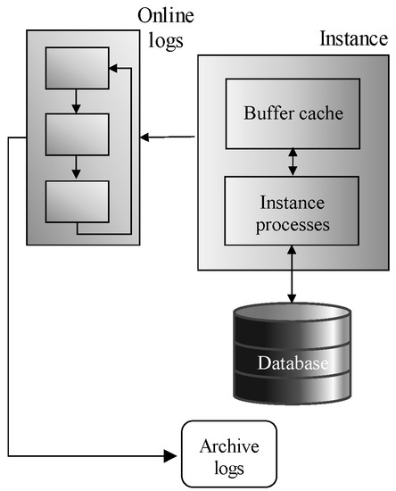
Figure 1.
Archivation architecture.
The reason for discussing log files is mostly associated with the usage in terms of temporality. The first solutions dealing with historical data were based on using log files to obtain historical data image. In principle, log files can be used to get the data image in the defined time point or even interval in the past. The prerequisite is just the completeness of the log files, otherwise, the reached object could be invalid, not covering the missing changes. If the log file list is complete, historical data can be obtained. Figure 2 shows the steps to get a historical image. The evaluation consists of four phases. In the first phase, the current data image is obtained. Then, online logs are applied to get the required time position (the second and third phase). They are operated by the instance background processes (Log Writer, Process Monitor, etc.). The process is physically modeled by two phases (second and third phase), whereas the log data are partially in the instance memory (for not approved transactions and in online log repository located in the physical the storage (for active and inactive transactions). Finally, an optional step is presented (the fourth phase), if the online logs do not cover the defined time point. In that case, archived log files are used, extracted, and applied to the objects. After processing, a historical data image can be obtained. The limitation is just the necessity to scan all log files sequentially, whereas individual states influence the consecutive state, it cannot be applied in parallel, directly. In [9,10], transaction operation precedency is discussed, by which just the most historical object is created, without the change monitoring. As the result, the historical image can be built sooner, and parallel data processing can be used, which dynamically improves performance. If the archive log mode is not enabled, historical data can be created in only a limited time manner [10]. Similarly, if any log file is not present, historical data cannot be obtained, at all. From the log header, it is not possible to detect, whether the particular transaction operates with the relevant object or not. Thus, all log files must be scanned in a time-ordered manner, even if they do not cover any change on the required object [8,10]. Even more, the particular object does not need to be part of the current data set, it could be removed sooner by the Delete operation [11]. In [12], another solution dealing with historical images was defined. The starting position does not need to be a current data image, any historical backup can be used, as well. The profit can be reached by reducing the amount of the logs to be applied promptly (logs are always sorted on time by the SCN value—System Change Number, which evolve sequentially). Figure 3 shows the processing data flow. In the first step, the nearest data image is obtained, provided either by the current image or the backup. If the backup is used, the whole data image has to be referenced (whole/complete/level 0 backup). In the third step, incremental backups can be applied, the preferred type is cumulative, however, incremental can be used, as well, but in that case, the individual object can be referenced multiple times by applying all changes over the time, which limits the performance strategy [13]. At last, individual logs are used—first archived and then online. Reflecting on the performance, there is an assumption, that the number of logs can be lowered by using backups. In [14], performance limitation is discussed, just with an emphasis on backup loading, which can be resource-demanding, as well. There are several enhancements of the log file management to cover historical images. Flashback technology can automate the process [10]. Extension to the Flashback data archive provides a robust solution by defining attribute sets, which have to be monitored over time. Thanks to that, the amount of the data to be parsed and evaluated is lowered. Principles are defined in [6]. Performance improvement of the Flashback data archive can produce object specification distribution, where the individual objects are divided into sets covering the range of attributes. From the performance point of view, it can bring noticeable performance improvements [15], however, a strong problem can arise there if the references across the distributive architecture have to be used, to ensure data consistency. In that case, several segments have to be notified to cover reliability and integrity. Note please, that the references can be created, reflecting the foreign keys. If any object created as the composition of other objects is changed, also the secondary objects need to be monitored, etc. [15,16].
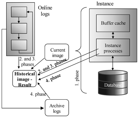
Figure 2.
Historical data obtaining process—the current image starting point.
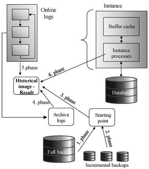
Figure 3.
Historical data obtaining process—the backup starting point.
Limitation of the above principles can be done by the temporal spheres. It is evident, that log files cannot cover the complexity of the temporal systems. Managing them requires parsing, which is too resource and processing time demanding. Moreover, if any log file is missing, the provided data can be compromised, providing incomplete and non-reliable data outputs [17]. Covering the possibility of data corrections, problems are even further [18,19]. From the temporal perspective, log management, not Flashback does not reflect the fullness of the temporality. Current valid data reflection is straightforward, they are directly present in the database. Historical data can be partially obtained by the logs, which are, however, stored in the file system, so the outside processes can manipulate them. The sharpest limitation is the impossibility to deal with the future valid data, prognoses, individual decisions influencing the objects in the future. Therefore, such models are mostly historical, not temporal in the whole perspective, the right part in the time spectrum is missing. Although some solutions dealing with future valid data management exist [20,21,22], the problem is just the relevance and up-to-date change reflection.
In this paper, we deal with the temporal data models in the various granularity levels based on the relational database form. It allows the use of relational algebra for the evaluation and processing, physical structure is delimited by the entities and relationships.
2.2. Temporal Database Architecture—Granularity Levels
The first conventional database approaches were released in the 1960s of the 20th century. It was clear from the solution that sooner or later it would be necessary to monitor changes in attribute values over time to create a temporal approach. The first solutions based on log file management do not provide sufficient power in terms of robustness, performance, and scalability. Historical images are stored in the log files as part of the database, but there is no direct access to them. Therefore, it is always necessary to process them sequentially and build a state valid in the past. From this point of view, history is stored externally, outside of effective management, and accessed by indexes. It is therefore clear that despite several improvements to historical databases [9,19,23] such a concept is unbearable in the long run. The essence of the temporal paradigm is the management of data in the entire time spectrum and the effectiveness of the process of building the image of the object, or the entire database within a defined time frame. The object-oriented temporal approach became the basis [10]. It was created by extending the primary key of an object. In this case, it is not enough to identify the object itself, as is customary in the environment of conventional systems, it is necessary to add information about the time expression. The representation of time can have several meanings, but typically as an expression of validity, the transactions, positions, etc., roles can be used, as well.
The architecture and principle of the system are shown in Figure 4. The first model represents a conventional—non-temporal model. Only current valid states are stored in it. If a change occurs, the individual versions are not reflected. The direct Update command is executed by which the original records are physically overwritten by the new ones. An overview of individual changes is thus lost. Individual data fixes and version control cannot be processed, at all. In terms of time, it is always just the current time image. The second model in Figure 4 is uni-temporal. The primary key is extended by a time interval modeled using the attributes BD (begin point of the validity) and ED (end of validity). Since the state identifier (primary key) is composite—it consists of the object identifier—ID (naturally, the object identifier itself can be composite) and the time limits—BD, ED, it is possible to record individual states positionally in time. The expiration date is often undefined from a logical perspective, but it is not physically possible to use a NULL value precisely because this attribute is part of the primary key and must hold real value. In principle, three solutions are used, either replacing an undefined value with another expression, usually a sufficiently large time representation (e.g., 31-12-9999 as the currently maximum modelable time point in the DBS) [10,14] or removing the expiration attribute from the identifier definition. In principle, this is technically possible, because the {ID, BD} pair itself must have a uniqueness property, as the time intervals for a particular object must not overlap. On the other hand, the time frame thus defined is not correct from a logical perspective. This is based on the original concept of the period data type. At present, the validity interval expressing the beginning and the end of validity is often modeled by two-time points, i.e., two attributes, but both are inseparable and interdependent. In the defined architecture, after removing the time attribute BD or ED, the temporality would lose its meaning. It would not be possible to define time positionally, nor to resolve collisions and undefined states [20]. The third solution was introduced in [3] and it is based on replacing undefined values with the specific pointers to the instance memory reflecting the data types. Thanks to that, particular values can be part of the index, and data retrieval efficiency can be ensured. In comparison with the default values replacing the undefinition, respectively in an unlimited time manner, there is no problem with the consecutive interpretation of the values. Moreover, such a concept can be used generally for any data type, which just limits the problem of designing a suitable value to replace an undefined value, both physically in the database and interpretation and indexing. Besides, it should be emphasized that using a different value to specify an undefined value requires additional disc requirements because these values must be physically stored in the database. The simplification of the second model in Figure 4 is a representation of a third object-oriented time model. Its representation is also shown in Figure 4 (last model). The time representation is expressed only by the beginning of the validity, and therefore each additional state automatically limits the validity of the direct predecessor. The primary key is again composite but consists of only two elements—the object identifier (ID) and the beginning of validity (BD). The advantage of the mentioned third model is the reduction of disk space requirements. On the other hand, in such a system, it is not possible to directly model and identify undefined states, these must therefore be defined explicitly [16,21]. Principles of undefined state management and identification are covered in [24,25] It must be stated either explicitly [16] or by pointing the state to the undefined memory locator [25] improving performance, whereas the whole state is grouped, whereas the object level granularity is used.
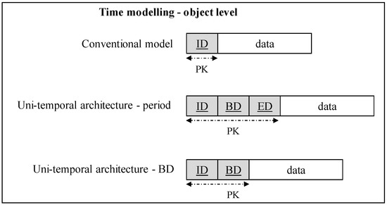
Figure 4.
Object-level temporal architecture.
Figure 4 shows only management in terms of the validity forming uni-temporal architecture. In general, multi-temporal systems can be used to model multiple time dimensions by allowing data corrections.
The attribute-oriented temporal approach is based on the mainstream system used within the temporal paradigm—object granularity, in which any change causes the creation of a new state, which may lead to the need to store duplicate values if some attributes do not change their values over time with each Update operation. This causes increased costs for disk space, processing, storage, and evaluation. In such a system, there are no direct links between the Update command and the attribute change. It requires the sequential comparison of individual values forming states, or versions of objects [26]. The aspect of value change also plays an important role here, with an emphasis on identifying a significant change. The minimum change in value may not be important for the system and may not need to be recorded in more detail [10,16,27]. In this case, it can be declared that the existing value expresses another state without change. The significant increase in the amount of data to be processed and its heterogeneity brought the need to create a new temporal architecture that could cover current trends, object volatility, sensory networks, and overall monitoring of object states throughout the time spectrum. The essence of the implemented solution is to move the granularity of processing to the level of the attribute. Thanks to this, individual changes are always associated with a specific attribute, the overall view of the object in a defined time is created by the composition of individual partial values of attributes. Principles are defined in [28]. Technology improvements of the temporal layer are defined [28] by correlating the same data type to the common group. The architecture consists of three layers. The first layer is conventional covering Current valid state images. Historical data and future valid images are in the third layer. Finally, the core element is supervised by the second layer (Temporal management). Any change is monitored and maintained by the temporal module. Each change of the attribute fires adding one extra row into the temporal table (located in the Temporal management layer). Architecture is in Figure 5. The left part of the figure shows the architecture and interconnection to the application. Blue arrows represent the data communication between individual layers. Whereas the whole communication is supervised by the Temporal management, future valid states cannot be routed to the current layer directly. Similarly, current states cannot be operated and marked as historical without the approval and acknowledgment of the temporal management layer. External applications can be mapped either into the temporal management (green arrow in the left part of the figure) or to the current valid states, as well (red arrows in the left parf of the figure). The reason to propose both techniques is based on the existing applications dealing with only current valid states. The aim is to offer the possibility to remain the original application without any change, only the flag to the temporal layer as the supervisor is done. Note, that the data provided is secured, thus the application cannot directly locate individual layers.
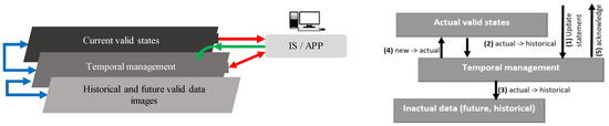
Figure 5.
Attribute oriented temporal model.
The right part of Figure 5 shows the data flow. If the new state is created, the system creates the Update statement of the existing state (1) by transforming existing state into the historical (by the assumption, that new state should be immediately valid). It is done by two phases—actual → historical (2) interconnecting current valid states and temporal management. The new state is inserted to the temporal layer. The original state is marked as historical and loaded into the third layer (3). Afterwards, the newly loaded state is denoted as current by the new → actual operation (4). Finally, the user or application gets the acknowledgement of the executed and approved operation (5).
By improving the structure, the way of manipulation, as well as the access methods, we found additional properties for optimization and thus increased performance. The next step was to create an extended approach for working with the extended attribute level temporal approach. The system is also based on the granularity of attributes (columns). The main difference is the modification of the temporal change table in the second layer—an explicit definition of the type of the executed command was added—the Insert, Delete, Update, or volatility methods. It is also necessary to think about the management of undefined states, their explicit definition, and transformation. In the case of the Update temporal statement, a numeric value for the data type category is also stored. Again, a three-level architecture is used, but only the first level remains unchanged, with the task of connecting to existing applications and accessing currently valid records. Historical data, resp. images of planned states are, in contrast to the previous solution, grouped based on the category of data types, the so-called basic types. Each category is assigned a table for storing attribute values. The primary key of this table is the numeric identifier (ID) obtained from the sequence and assigned by the trigger. The next attribute contains the value of the data type of the relevant category it represents. The overall system is managed using the proposed semantics—algorithms of triggers, procedures, and functions. Although additional attributes are added to the changing table, increasing the disk space requirement, the execution of the Select statement is significantly streamlined, simplifying the identification of the change made and the state construction process. The required number of tables for historical data is also significantly reduced. If the original columnar approach given as we stated were used, another (separate) table would be defined for each temporal attribute, in which case, 4–5 tables will often suffice, depending on the characteristics and structure of the stored temporal value. We use the term base core data type. It combines specific data types implemented in the data model into common categories. For example, numeric representations of Integer, Number, Float can be categorized together as type Number. The chain characteristics are covered by the basic type Varchar2 (max). Thus, for example, separate tables do not have to be defined for the real data types Varchar2 (20) and Varchar2 (30), the values of outdated states can be combined. In addition, the attributes expressing the date and time can be implemented together as a timestamp with the appropriate precision. The temporal layer on the second level consists of the following attributes:
- Id_change—primary key, the value of which is set using a sequence and a trigger.
- Id_previous_change—the value is obtained as the maximum value of the ID_change attribute for the object identified by ID_orig in the relevant table (ID_tab). If it is a new object, the attribute will be NULL.
- Statement_type determines the type of command executed:
- ○
- I = Insert.
- ○
- U = Update.
- ○
- D = Delete (physical deletion of the historical record from the system).
- ○
- P = Purge (removal of historical states in terms of their transfer to external archive repositories, extended by an optional transformation module (anonymization, aggregation, etc.)).
- ○
- X = Invalidate (creation of a complete undefined state of an object preceded by moving the object as such under the management of undefined objects).
- ○
- V = Validate (also known as Restore)—restoring an invalid object and replacing its state with an applicable one that meets all integrity restrictions.
- ID_tab—identifier of the table in which the change occurred.
- ID_orig—attribute that carries information about the identifier of the changed row.
- Data_type—an attribute that defines the basic data type of the changed temporal attribute (the real data type can be obtained from the image of the data model valid at the defined time instant):
- ○
- C = Char/Varchar2,
- ○
- N = numerical values (Real, Integer, …),
- ○
- D = date type Date,
- ○
- T = Timestamp,
- ○
- L = Lob,
- ○
- X = XML, etc.
- ID_column—refers to a temporal column whose values change.
- ID_row—associates the table with historical data (if the Update command was executed, otherwise it is NULL).
- BD—time value expressing the beginning of the validity of the new state.
2.3. Proposed Improvement
The limitation of the attribute level temporal system defined in the previous paragraph is correlated with the effectiveness of the Update statement. If multiple attributes are updated at the same time, each of them requests inserting a new row into the temporal layer, which creates performance limitation and the bottleneck of the whole system. Group level temporal architecture is based on synchronization groups detection. The managed granularity of the temporal layer can be either the attribute itself or the whole synchronized group, which is detected and managed automatically. Figure 6 shows the architecture. Black arrows show the data flow during the synchronization group detection. Input data are analyzed in the first phase. If any relevant synchronization is detected, the Group manager is contacted (2). In the third phase, the new group is created and its temporal definition is stored in the temporal management (4). The red arrow represents the input data stream to the system. In comparison with the attribute oriented solution, external systems cannot access actual valid states directly, whereas the group detection would be avoided.
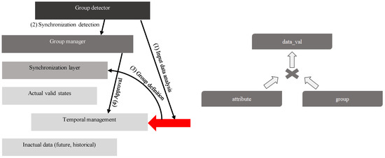
Figure 6.
Temporal data grouping—solution architecture.
In this paper, we propose the extension of the group level temporal architecture by shifting the processing to the second level. Data themselves are not synchronized only in a time manner, by the positional data are taken care of. Individual data are segmented into categories by the added layer specifying data positions. The defined area is divided into individual polygons, which form the non-overlapping regions. From the interface point of view, temporal and spatial data are managed either separately, or the whole spatio-temporal perspective can be used. Each attribute can be managed either separately or can be formed into the group by covering multiple attributes, which are updated synchronously. In that case, it brings the benefits, whereas the whole group (which is dynamic and its validity is temporal, as well) is referenced in the temporal layer, not just individual attributes. In principles, if the group is composed of 5 synchronized attributes, only one Insert statement is performed in the temporal layer, instead of adding 5 new rows. The temporal aspect, however, does not need to be the only layer of processing and data grouping. In the proposed solution, spatial architecture can be used, as well. Many times, namely, data are produced and transferred using the ad-hoc network with specific reliability, speed of the transfer, and failure resistance. Therefore, individual data can be grouped based on the positions forming the complex data image with the defined granularity and frequency.
Architecture is in Figure 7 extending the temporal concept by the spatial reference. In comparison with the core group level system, the interface is extended covering the spatial positions and categorization. Note, that the region definition can evolve and the temporal layer must reflect the structure changes.
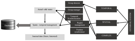
Figure 7.
Spatio-temporal grouping.
3. Transaction Support and Integrity
The essence of relational data processing is transaction ensuring the transformation of the database from one consistent state to another. After the processing operated inside the transactions, the stored values are correct and meet all defined rules and integrity constraints. Temporal reliability and consistency are essential elements of processing. As the characteristics and requirements of the temporal system evolve, individual transactions must reflect changes at the level of the current data model and integrity constraints.
The task of conventional databases is to process currently valid data, when changing them, the Update command is physically executed, after executing the Delete command, the relevant records are deleted from the database, and information about their existence is lost from the main structure, even though this information is partially available in backups and log files. In the case of temporal databases, individual changes are implemented using the Update and Delete commands only at the logical level, the data are physically updated in the form of creating new states. Therefore, if an event occurs in which the state of the object needs to be changed, the original record is bounded by validity and a new record is inserted. All changes are covered by relational theory and transaction management, which is characterized by the following properties defined for the conventional approaches. In this paper, we extend the defined rules (ACID) by the following representation for each category [4,29]:
- Atomicity—generally, the transaction manager must guarantee that the transaction will be executed either in its entirety (execution and approval of the transaction using the Commit command) or no part of it will be executed (Abort or Rollback command). In the temporal perspective, dealing with higher security demands, any state is stored into the database, even if it is consecutively rollbacked, removed, or corrected. Temporal dimension in the proposed solutions use the flags, so the transaction representation can be used widely.
- Consistency—this feature requires that confirmed changes are permanent, even in the event of an accident. This means that changes must not only be persistent but also renewable. This is ensured by the transaction manager using the Log Writer process, where each change is logged with an emphasis on the created image before and after the operation. Thanks to this, it is not necessary to apply the changes physically over the data blocks of the database, but it is enough to change the data in the memory (buffer cache) and at the same time, record the change physically in the log files in the database. At the same time, the temporal world emphasizes the speed of disaster recovery, so changes are cumulatively written from memory to the physical database to minimize time and technical complexity.
- Isolation—the requirement of isolation is based on the fact that the changes are published and available to all only if the transaction itself is confirmed. Therefore, it cannot happen that another transaction will access data that will later be canceled, as the transaction would be rejected. Another problem with isolation is the reconstruction of historical conditions. In terms of versions and transactional recovery, a Snapshot too old exception often arises in conventional systems [4]. This problem occurs when a transaction needs to obtain object state images before another transaction can commit the change. However, such original states may no longer be available and may not be recoverable from transaction logs. In a temporal database environment, the problem can be even more pronounced because the system contains a large number of changes covered by many transactions, and these changes are dynamic, updating the database with different time granularity, often down to the nanosecond level. Therefore, it is necessary to emphasize the possibility of restoring transactional versions.
- Durability or correctness in other words. Transactions must verify in the approval process that they are processed correctly and that they meet all integrity constraints, which may, however, change over time. The transaction manager, with the support of other instance processes, constructs a data model valid at a given time and applies integrity constraints to it, against which the inserted records are verified.
3.1. Proposed Extension—Data Reflection
The already defined types as the extensions of the conventional approach are not suitable for the temporal manner. During the research in the temporal sphere, we came to a significant problem, which is not covered by those categories complexly. Therefore, in this paper, we introduce the Data reflection category. Data in the temporal system are stored for a long time. The above principles, however, do not reflect the possible changes in the structure, as well as the evolution in the constraints definition. Multiple sources and data origins are consecutively added to the temporality, therefore the demand for the structural changes is present and required almost always. For the temporal evolution, just the changes in the data model can be placed, so the state must reflect the particular data model defined in the validity time frame. Note, however, that the data model can be changed during the valid data state itself. Similarly, the state can be defined with the future planned validity, however, data model reflection must be done directly during the transaction processing sooner in a timeline manner. As the result, the transaction only reflects states referencing the “AS-IS” data model, however, the validity is shifted to the “AS-WILL BE” model. Thus, the particular state can be approved with the temporal reflection. Physically, before getting the validity state mark, a particular model is checked, whether all constraints are there passed or not. For suitability and completeness, any change, even done automatically during the transaction shifting, is monitored and stored in the temporal layer by the flags. The state itself can hold the following status:
- Valid—the state is currently valid or has been planned in the past by moving the state into the valid representation currently.
- Corrected—the state was planned and later state values were corrected (mostly by using bi or multi-temporal architectural model).
- Transaction refused—the planned state was removed as the consequence of breaking any of the concerning integrity rules.
- User rollbacked—the whole transaction is user rollbacked.
- Refused—the state does not cover the already planned model in the future.
- Planned—the state is planned to be valid in the future, the particular model is not defined yet, or all conditions reflecting it are passed.
- Modified—this option reflects the transaction rules, by which the original state validity is changed, either shortened or shifted in a timely manner.
3.2. Conventional Log Ahead Rule (LAR)—Existing Definition
The database object can be modified only when the changes are recorded in the logical journal (log). This rule allows the transaction to execute an UNDO operation in the event of an interruption. Because all changes are recorded in the logical journal, it is always possible to return the database to its original state at the beginning of the transaction. Additionally, in the event of an incident, these transactions can be restarted. The change itself then takes place in the memory structures of the instance, specifically in the Buffer cache, the contents of which are then written to the database (by the Database Writer process).
3.3. Temporal Log Ahead Rule (TLAR)—Proposed Solution
In the environment of the temporal approach, however, this rule is not so complex and does not cover the specification precisely because of the need to resolve conflicts, which newly created states can cause. The state change request is stored in a logical journal, however, before the database itself is updated, a transaction and integrity rule check is required, which is based on the fact that any object can never be defined by more than one valid state. Therefore, if necessary, the transaction rules are applied and the validity period is adjusted for the existing or new status.
3.4. Extended Temporal Log Ahead Rule (ETLAR)—The Proposed Extension
In this paper, we propose an extended solution for the TLAR covering the particular data model, as well. Thus, in the first phase, data are logged regardless of the constraints. Thanks to which all changes are preserved, regardless of their correctness and applicability. Secondly, state overlapping is detected, covered by the TLAR, as well. As stated, any object can be defined by just one state anytime. The third phase evaluates the data model. The data model can evolve by extending, adding, or dropping existing constraints. Data attributes and integrity can be enhanced, as well. Thus, each database element is determined by the activity time frame, to which it belongs. Data model image is then composed as applying all data model segments, which are valid in the defined time positions. In conventional systems, the Two-Phase Commit protocol ensuring transaction durability and whole process reliability is used [10,11]. It is based on the logging, by which any data portion should be placed in the logs before the change itself. For the temporal environment, log management was extended by collision detection and management forming the Three-Phase Commit protocol. In this paper, we propose Four-Phase Commit protocol (4PCP) to manage the data model covering, as well. Figure 8 shows the data flow. The first step is associated with the transaction logging in the autonomous transaction, thus even after the main transaction refuse, objects are present in the temporal layer, however, just with the User rollback flag. Afterward, consistency reflecting the data model is measured. If the new state temporality reflects state immediately valid, respectively data correction to the historical data images, “AS-IS”, respectively “AS-WAS” model can be used, reflecting the data model valid in the defined time point or interval. Transaction control can evaluate, whether the states fulfill all the requirements and all constraints are passed, even if multiple data models are valid during the time interval. Dealing with future valid data is, however, far more complicated. First of all, the “AS-IS” approach cannot be used, whereas it must reflect conditions in the objective time frame denoted by the validity. In ideal conditions, the particular data model is available, thus the transaction can evaluate and reflect either data model, as well as all constraints. Thus, the “AS WILL BE” delimitation can be done. Vice versa, if the data model is not defined for that moment or time frame, evaluation cannot be done, transaction control cannot manage constraints, at all. In that case, the transaction has ended successfully and constraint management is shifted to the time, the data model is present and properly defined. By specifying a new data model or changing environment, the original transaction can be reopened to notify the data model. As the result, the originally conditionally approved transaction is reevaluated. Naturally, dependent objects can be identified in other transactions, thus the constraint checking does not need to cover only one transaction, however, the transaction chain can be necessary to be reevaluated. The temporal layer comes to the solution of the problem, which covers all the changes, even refused or corrected. By referencing time and transaction pointers, it is always possible to ensure data correctness and consistency, if any metadata characterizing conditions or environment is changed. Figure 8 shows the evaluation data flow in the UML diagram. The first phase is delimited by the logging until reaching the Ready to Log (RL) data point. The second phase deals with collision management. State overlapping is managed regarding the defined rules. The transaction timeline is bordered by the Ready to Transaction Collision (RT) point. Data model reflection checking is done in the third phase, ensuring that all constraints will be passed in the future valid model, if available. It is delimited by the Ready to Model (RM) point. Finally, in the fourth phase, data are shifted into the database, and the transaction is approved reaching Ready to Commit (RC) and the transaction is ended (EOT). Begin point of the transaction is denoted by the BOT.
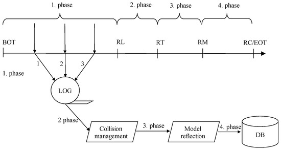
Figure 8.
Four-phase Commit protocol.
This paper extends the principles covered by the paper proposed in the conference FRUCT 27 placed in Trento (Italy) [16]. Such contribution aimed to deal with the transaction rules to ensure data state reliability. It must be always ensured, that each object is defined directly by one state. A collision occurs if multiple states of one object are to be valid at the same time. Such a situation is identified by the transaction manager and several rules can be used to limit such problems. In [16], several access rules were presented: complete reject (adding new state, which overlaps the existing or planned state is refused completely), complete approval (removes the impact of the already planned state by removing it totally), partial approval (delimits the new state and shortens its validity to remove overlapping problem), or reposition (moving planned state to another time dimension).
4. Indexing
A database index is an optional structure extending the table and data definition offering direct data location, whereas the data address locators (ROWID) are sorted based on the indexed attribute set. By using the suitable index, data can be located by examining the index first followed by the data location using ROWIDs. It is the most suitable and fast method, in comparison with the whole data block set scanning (Table Access Full (TAF) method), block by block sequentially until reaching the High Water Mark (HWM) symbol. It denotes the last associated block of the table. Generally, data blocks are not deallocated, even if they become empty, due to the management requirements, performance, and resource demands [30,31]. It does not have negative aspects in the terms of the storage and overall estimation, whereas there is an assumption, that the blocks will be used soon in the future, so they are already prepared. When dealing with Table Access Full, the empty block cannot be located directly, whereas the fullfillness is nowadays stored directly in the block itself. In the past, data blocks were divided based on the available size and split into particular lists, which were stored in the data dictionary. The limitation was just the necessity to get the data from the system table, which created the bottleneck of the system [9,32]. If the system was dynamic with frequent data changes and inserts, the problem was even deeper.
When dealing with the index, only relevant data blocks are accessed. They must be loaded into the memory using the block granularity and data are located, again by using ROWID values, which consist of the data file, particular block, and position of the row inside the data block. Thanks to that, data are obtained directly, however, one performance problem can be present, as well. In principle, data after the Update operation are usually placed into the original position in the database. Thus, the data ROWID pointer is not changed and remains still valid. If the data row after the operation does not fit the original block, the newly available block is searched for or even allocated forming a migrated row. It means, that the ROWID value remains the same, but inside the block, an additional reference to another block is present. As a result, in the first part, the data block, to which the ROWID points is memory loaded followed by getting another block, where the data resist. Thus, two blocks are loaded, instead of just one. Generally, data can be migrated multiple times, resulting in the performance drop caused by the huge amount of I/O operations. Although the index can be rebuilt even online, it does not provide sufficient power due to the problem of dynamic changes across the data themselves [33].
In the relational database systems, various types of indexes can be present, like B+tree, bitmap, function-based, reserved, hash, etc. [1,34]. The specific category covers string indexing and full-text options. Temporal and spatial indexes have the common index types, however, almost all of them are based on the B+tree indexing, which is also the default option, as well. B+tree index structure is a balanced tree consisting of the root and internal nodes sorting data in a balanced manner. In the leaf layer, there are values of indexed data themselves, as well as ROWID pointers. Individual nodes are interconnected, thus the data are sorted in the leaf layer across the index set. To locate the data, index traversing is done using the indexed set resulting in either obtaining all data portions needed or by obtaining ROWID values, by which the other data attributes can be loaded easily (executing Table Access by Index ROWID (TaIR) method. Reflecting the data integrity, it is always ensured, that any data change is present in the index after the transaction approval. There is, however, one extra limitation associated with the undefined values. They are commonly modeled by using NULL notation, which does not require additional disc storage capacity. Whereas NULL values cannot be mathematically compared and sorted, NULL values are not indexed, at all [24,35,36]. Although the database statistics cover the amount of the undefined values for the attribute, they do not reflect the current situation, just the situation during the statistics were obtained, thus they cover mostly background for the decision making in terms of the estimation. Management of the undefined values inside the index is currently solved by the three streams. The first solution is based on the default values, which replace the values, which are not specified [4,26]. The problem causes just the situation when the NULL value is specified explicitly. In that case, the default value cannot be used. The complex solution can be provided by the triggers [6], replacing undefined values. From the performance point of view, there are two limitations, first of all, it is associated with the trigger firing necessary, which must occur for each operation. In the temporal environment, where a huge data stream is present, it can cause significant delays and reliability issues. Second, default values are physically stored in the database, thus it has additional storage capacity demands. Finally, undefined values can origin from various circumstances, thus undefined values can be represented by the numerous default values expressing e.g., undefined value, delayed value, inconsistent value, non-reliable value, the value of the data type range, etc.
Function-based index removes the impact of the additional storage demands, on the other hand, there is still the necessity to transform the value regarding the reasoning resulting in non-reliable data if the categorization cannot be done. Therefore, the solution extends the attribute specification defining the reason and representation of undefined value. From the point of view of the physical solution, we finally come to the interpretation of default values [6] with no benefit.
Regarding the limitation of the existing solution, we propose another representation in this paper. Our proposed solution is based on the model of undefined value management covered in the index. The core solution is defined by our research covered in the MDPI Sensors journal [28]. It deals with various circumstances and models for dealing with undefined values. Several experiments are present, dealing with temporal, as well as spatial databases. Principles are based on adding a pre-indexing layer used as the filter. If the undefined value is located, its pointer is added to the NULL module connected to the root element of the index. Thus, the original index dealing just with valid defined data is still present, but undefined values can be located from the root, as well. The data structure for the NULL module representation was first defined as a linear linked list with no sorting, which brought the performance improvements in the Insert operation, whereas there was no balancing necessity, on the other hand, such data would be necessary to totally scan. In the next step, therefore, the module representation was replaced by the B+tree, in which the data were sorted in an either temporal or spatial manner. The final solution was based on the spatio-temporal dimensions formed by two-pointer stitched indexes, the first is temporally based, the second reflects the associated region, thus not the data positions are indexed, just the reference to the particular region. Another solution was based on the region of temporal dimension partitioning.
4.1. The Proposed Solution—NULL Value Origin Representation
The limitation of the already proposed definitions is just based on the NULL value notation. It is clear, that there are no additional size demands, however, there is a strict limitation of the representation. We, therefore, developed another solution proposed in this paper as an extension of the current solutions. As stated, the undefined value can be physically associated with the various circumstances, like delayed value, improper value, the value provided by the compromised network, etc. There is therefore inevitable to distinguish the reason, undefined value itself is not feasible. The architectural solution reflecting the model is the same in comparison with [28], thus the second level indexing for the temporality (first dimension) and spatiality (second dimension) is used. For this solution, undefined values are also categorized based on origin. Categories can be user-defined, or automatic segmentation can be used. To create a new category for the undefinition, the following command can be used. The name of the database object must be unique among the users. It is associated with the treating condition specified similarly as the Where clause of the Select statement is defined. Multiple conditions can be present for the representation, delimited by the AND and OR connections. Moreover, the same condition can be used in multiple definitions, as well. In that case, the undefined value is categorized by multiple types and present in the index not only once. Physically, it is modeled by using ROWID pointers, thus the object itself is used only once, but several addresses (similar to the standard indexing) can point to that:
- Create null_representation name defined as condition;
For dealing with the delayed data caused by the network, the following notation can be used:
- Create null_representation network_delay defined as sent_time—received_time > 3 s;
For dealing with the delayed data caused by the database system interpretation, the following notation can be used:
- Create null_representation network_delay defined as received_time—processed_time > 1 s;
The definitions are stored in the data dictionary—null_representation prefixed by the user (only objects created by the current user), all (created by the user or granted to him), or dba (covering all definitions across the database instance). They can be granted to multiple users via grant command:
- Grant usage on name to user_list;
After the NULL representation creation, the definition is put to the data dictionary, so they can be associated with the defined tables, respectively, attributes or the whole database can be used. The whole representation model unioning the set is used, thus, if the representation is defined for the whole table, it is automatically granted to each attribute, which can hold undefined value. Moreover, the definitions can be extended by the attribute reflection, as well. It is done by the following syntax:
- exec dbms_null.assoc_tab(table_name, null_representation_name);
-- for dealing with the table
- exec dbms_null.assoc_attr(table_name, attribute_name, null_representation_name);
-- for dealing with the attribute
- exec dbms_null.assoc_db(username, null_representation_name);
-- for dealing with the user
Note, that if the username is not defined in the last command, the current user executing the code is used, by default.
Figure 9 shows the proposed architecture consisting of three core internal elements. The Management handler is responsible for associating NULL representation, to interconnect undefined value categories (NULL_representation) stored in the data dictionary with table data by the definition. Any used category is created as the separate elements in the memory, (NULL_representation memory pointer layer) to which individual data can be directed. The second internal element is just the Index module storing the whole data set (even NULL values are there, in the separate storage segment in B+tree index stitching by the three layers—spatial, temporal, categorical). The categorical definition is based on the pointers to the NULL_representation memory pointer layer, by which the type and origin of the undefined value are present. If any change on the NULL_representation, either in the data dictionary or the table association is done, the Management handler becomes responsible for the change to apply it to the whole structure. Data input stream layer (Data change module) is the input gate for the data changes, it is modeled by the separate module, where the pre-processing, filtering, and other reliability and consistency operations can be executed. Data retrieval is done straightforwardly from the Index module, as well as the database itself. The architecture of the solution is in Figure 9. Core internal elements are gray colored. External modules are either represented by the database itself or by the data dictionary object. Green part represents database and external systems, to which the result set is provided. Dotted arrow separates the data dictionary from the instance itself.
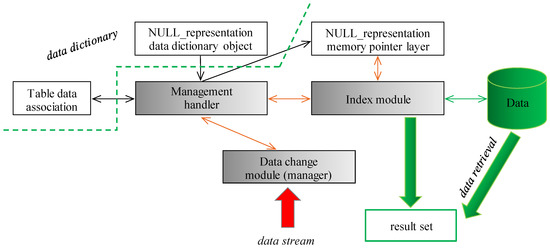
Figure 9.
NULL categorization model—proposed architecture.
4.2. Proposed Solution—Master Index Extension & Partitioning
When dealing with index structures, various access methods can be used to locate data. Index Unique scan (IUS) is used if the condition reflects the unique constraint by using an equality sign. If the multiple values can be produced, either as the result of the range condition or by using the non-unique index, the Index Range scan (IRS) method is used, naturally, if the order of the attributes in the index and reflecting the query is suitable. There are also many other methods, like Full Scan based on the fact that the data are already sorted in the leaf layer, so the ordering is not necessary to be performed, Fast Full scan, where all suitable data are in the index, however, the attribute order forming index is not suitable, thus the index is scanned fully. The specific access path is defined by the Skip Scan, which can be preferred if the query lacks the leading attribute of the index. It is based on the index in index architecture for the composite definition [16]. As stated, if the index is not suitable or even if there is no index covering the conditions, at all (e.g., supervised by the function call), the whole data block set associated with the table must be searched by executing the Table Access Full method. It can have many severe limitations and constraints, mostly if there is a fragmentation present if the associated block amount is higher in comparison with current real demands. All of these factors have significant performance limitations. The Master index was firstly defined in [24]. It uses the index just as the data locators. Generally, any index structure can be used, holding any data. By using the proposed techniques covering NULL values inside the index, any index type can be used. The spirit of the Master index is to locate data by extracting the block identifier from the ROWID values in the leaf layer. Thanks to that, just relevant data blocks are accessed. Migrated rows are secured, as well, although the ROWID pointers are not used to address them, however, there is a pointer inside the block, which is associated with the index itself, thus the security and whole data frame can be accessed forming a reliability layer. If at least one record is pointed to the block, it is completely loaded and the whole block is scanned for either data themselves or for locating migrated rows. It removes the limitation of the memory Buffer cache problem covered in [9]. Specific index structure can be used, as well, based on the B+tree data structure, however, it points only to the data block, not the direct row position. Leaf layer automatically removes the duplicate pointers by sorting the data based on the index set, as well as pointers. A proposed solution dealing with NULL can be used, as well, individual categories are used in the separate module, in which the block definition pointers can be used, as well. The architecture of the Master indexing extended by the NULL pointer module categorization is in Figure 10. Communication interconnection of the modules is black colored, data flow in individual phases is shown green. The processing consists of several phases. The first phase represents the query definition and its representation in the database system. Server process of the instance memory is contacted (first phase), where the syntactic and semantic check is done. In the second phase, the existing index set is processed to identify a suitable index to access the data. The third phase represents the decision. If the suitable index to cover the query exists, processing is shifted to the fourth phase, the particular index is used and result set is created. Vice versa, if there is no suitable index to serve the query, the Master index module is contacted to select the most suitable index. Such index is used for the relevant blocks holding data extraction in the fifth phase.
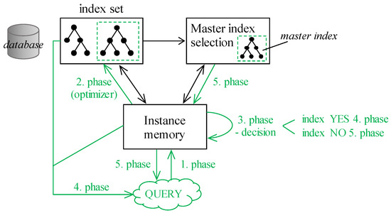
Figure 10.
Master indexing.
Partitioning enhances the performance, manageability, and availability of a wide variety of applications. It is useful in reducing the total costs of the ownerships and storage demands if a large amount of data across the temporal and spatial sphere is present. It allows you to divide tables, indexes, and index-organized tables respectively into smaller pieces, enabling you to manage these objects at a finer level of the accessing and granularity itself. When dealing with the data access using the proposed stitching architecture leveling data to the temporality, spatial dimension, and undefined value categorization, partitioning can provide a significant performance benefit. Generally, data reflecting the continuous time frame is required, thus particular data are either in the same partition fragment, or the neighborhood is contacted. Similarly, positional data are obtained by the same region. The partitioned model differentiates individual values into the partitions based on the data indexes, the supervising background process Partition_manager is launched, which is responsible for the changes and overall architecture. Note, that each data portion can be part of just one partition in the same level, except the undefined values themselves. As stated, by using the null_representation object, the undefined value can be categorized into several types, resulting in placing the object into multiple partitions. For ensuring performance, the undefined value is determined just by one state represented to the memory module, thus it does not impact performance, at all.
4.3. Complex Solution—Autoindexing and Post-Indexing
In [37], the concept of autoindexing is proposed. It is based on the autonomous evaluation of the individual queries, by analyzing statistics, impacts, with emphasis on the current index set. The principle is based on the invisible and virtual indexes analyzing benefits and costs, if dropped [38]. The aim is to balance the existing index set to provide robust and fast access to the data during the retrieval process, but it takes emphasis on the destructive DML operations (Insert, Update, and Delete) as well. Our defined solution covering undefined values, a master index, and partitioning can form the core part of the autoindexing, as well, mostly in cases of dynamic queries and dynamic data changes over time. By extending autoindexing with the proposed methods, just peaks during the evaluation can be dropped, whereas the Table Access Full method can be replaced by the Master index, undefined values are part of the index in the separate layer interconnected with the root element. Thanks to that, a complex environment can be created. A complete overview of the architecture is in Figure 11. The current index list is present for the optimizer evaluation. Indexes are enhanced by the modules representing undefined values by the categories, which can evolve. The Master index is responsible for limiting the TAF method, thus the data fragmentation does not bring any limitation, at all, whereas empty blocks are automatically cut from the processing by using block identifiers (BLOCKID) extraction. As present in the experiment section, all the modules can bring additional performance power, creating a complex environment covering data access to the physical location. In Figure 11, there is also a module dealing with post-indexing. The purple part of the figure expresses the database statistics obtained from the database and index set. It is the crucial part, whereas without non-current statistics, reliable performance cannot be ensured. The green part shows the autoindexing module. The autoindexing process is interconnected with the optimizer and DB statistics. It uses internal Query evaluation costs/benefit module responsible for creating and removing existing indexes (black arrow between index set and Query evaluation costs/benefit module. Blue part represents the post-indexing process modeled by the Notice list structure and the Post-indexing process itself. The dotted arrows represent the data flow and interconnection. Post-indexing process regularly (or based on the trigger) checks the Notice list and applies the changes by the balancing. It is connected to the optimizer.
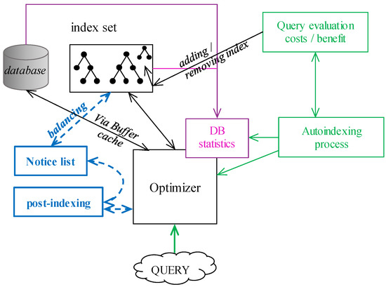
Figure 11.
Autoindexing + post-indexing module.
Transactions must deal with the logging to ensure ACID properties ensuring durability after the failure, but the aspect of the consistency and ability to rollback transaction is inevitable for the processing, as well. Data themselves are operated in the second phase, which covers the index management, as well. If any indexed object state is modified, change must be reflected in the index. Otherwise, the index set would be non-reliable and unusable in the result. Post-indexing is another architecture improving the performance of the destructive DML. B+tree index is namely always balanced, thus any change requires balancing operations, which can be remanding and form a performance bottleneck. In the post-indexing architecture layer, index balancing is extracted into the separate transaction supervised by the Index_balancer background process. In that case, individual changes are placed into the Index Notice list. Thanks to that, the transaction itself can be confirmed sooner. Although the balancing operation is extracted, it is done almost immediately. Moreover, it benefits from the fact, that changes done by the same objects can be grouped and operated together, although they originate from multiple transactions. Thanks to that, in total, performance benefits, multiple operations are applied to the index during one operation, followed by the balancing. Thus, balancing is not done for each change, they are bulked. Vice versa, data retrieval operations must deal not only with the index itself, but the Notice list must also be scanned, as well, to create a consistent valid object. Figure 12 shows the process of data retrieval. Note, that it can be done in parallel.
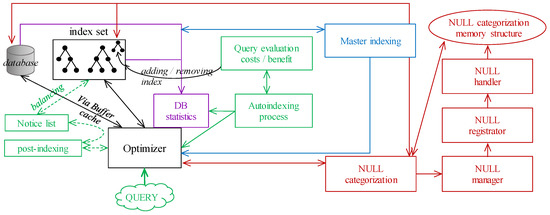
Figure 12.
Data retrieval—complex management.
5. Data Retrieval
The Select statement is considered to be the most important and most frequently used SQL statement, which is used to select records from the database, either from just one or more tables or views, respectively. The basic conventional syntax of the Select command consists of six parts—Select, From, Where, Group by, Having, and Order by [1,4]:
| [CREATE TABLE table_name AS] |
| SELECT [ALL|DISTINCT|UNIQUE] |
| {*|attribute_name|function_name[(parameters)]} [,...] |
| FROM table_name [table_alias] [...] |
| [WHERE condition_definition] |
| [GROUP BY column_list [function_list]] |
| [HAVING agg_function_conditions] |
| [ORDER BY column_list [function_list] [ASC|DESC] [,...]] |
Proposed Select Statement Definition
The temporal extension of the Select statement brings an important aspect of performance. It is a cross-cutting solution of all temporal models and is based on the temporal database paradigm, which requires that user perspective and result approaches to be the same, regardless of the physical internal architecture. The proposed solution extends the definition by the following clauses:
- Event_definition
This definition extends the Where clause of the Select statement, specifying the time range of data processed and retrieved, either in the form of a precise time instant (defined_timepoint) or a time interval (defined_interval), the definition of which contains two-time values—the start (BD) and end point (ED) of the interval. In the session or instance respectively, it is possible to set the type of interval (closed-closed, closed-open representation), but the user can also redefine the set access directly for a specific Select command. The second (optional) parameter is therefore the interval type used (CC—closed-closed, CO—closed-open). Note, that current database systems offer period definition by the name notation, it can be used, as well. It that case, the clause uses only one parameter, whereas the period data type always reflects CC representation:
- defined_timepoint (t)defined_interval (t1, t2, [CC|CO])defined_interval (period_def)
The output manages individual validity intervals, if at least one timepoint is part of the defined time frame, particular state is present in the result set. Figure 13 shows the representation and usage of the CC input validity interval (expressed by the period data type physically). Note, that the database states do not need to pass the CC interval definition, thus they are automatically transformed, by using Allen relationships and transformation principles [6]. Figure 14 shows the similar solution dealing with CO validity time frame. Specific type of the interval is denoted just by one timepoint. The following code shows the transformation of principles to the existing syntax, BD, ED express the inner database values, t1 and t2 represent validity intervals inside the Select statement definition:
| defined_timepoint(t) | where BD ≤ t AND t ≤ ED | CC internally |
| defined_timepoint(t) | where BD ≤ t AND t < ED | CO internally |
| defined_interval(t1,t2, CC) | where BD ≤ t2 AND ED ≥ t1 | CC internally |
| defined_interval(t1,t2, CC) | where BD ≤ t2 AND ED > t1 | CO internally |
| defined_interval(t1,t2, CO) | where BD < t2 AND ED ≥ t1 | CC internally |
| defined_interval(t1,t2, CO) | where BD < t2 AND ED > t1 | CO internally |
| defined_interval(period_def) | where BD ≤ t2 AND ED ≥ t1 | CC internally |
| defined_interval(periof_def) | where BD ≤ t2 AND ED > t1 | CO internally |
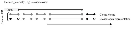
Figure 13.
Event definition—Closed-Closed model.
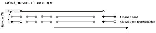
Figure 14.
Event_definition—Closed-Open model.
- Spatial_positions
When dealing with the spatio-temporal model, it is inevitable to cover the positional data and categorize them into the defined bucket set. When dealing with data retrieval, it is important to emphasize data correctness, relevance, and measurement precision. Missing data can be usually calculated by the neighborhood data positions, however, it is always necessary to mark such values and distinguish the measured data set from the assumed or calculated, respectively. Spatial_positions clause allows you to define an either polygon, which will delimit the data positions or radius. In this case, the data measurement frequency and precision are significant, whereas the data stream is not continuous, thus the object can be placed in the defined region just in a small term, however, such data should be placed in the result set, as well, to compose complex and reliable output. As stated in the previous chapter, the whole data map can be divided into several non-overlapping regions, which definition can be part of the proposed clause, as well.
- Spatial_positions (polymon_def)Spatial_positions (latitude_val, longitude_val, radius_val)Spatial_positions (region_def)
Definition of the region can be done for the whole database, user, or table association.
- Create region_representation name defined as {definition|polynom};
For the evaluation, the precision level can be specified holding the following options:
Precision_level:
- only measured data,
- measured and calculated (estimated) data,
- fuzzy classification of the assignment defined by the function.
Another relevant factor is delimited by the time duration (time_assignment), during which the object was part of the defined region, polygon, or point with radius delimitation, respectively. This clause can be extended by the optional parameter dealing with the time duration using Interval data type—Interval Day to Second (syntax is shown in Figure 15) or Interval Year to Month (syntax shown in Figure 16) [39]:
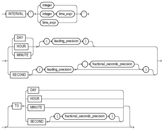
Figure 15.
Interval Day to Second—syntax [39].
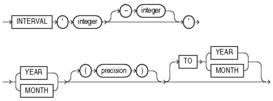
Figure 16.
Interval Year to Month—syntax [39].
The complex definition of the Spatial_positions clause is defined by the following structure. Note, that the data assignment to the defined region is different from the event_definition clause, in principle. In this case, namely, assignment granularity is used with the reflection to the spatial positions, whereas the event_definition deals with the whole time range of the data to be obtained:
- Spatial_positions(spatial_data_bordering [precision_level, time_assignment])
- Transaction_reliability
The purpose of the Transaction_reliability clause is to manage and retrieve individual versions of object states over time. The required architecture is bi-temporal, resp. a multi-temporal system that allows you to define, modify, and correct existing states using transactional validity. So it is not only the validity itself that is monitored, the emphasis is also on the versions and later data corrections. In principle, any change to an existing situation must result in the termination of its transactional validity. The new transaction validity is expressed by the transaction itself, its beginning is identical with the beginning of the transaction, the end of validity is unlimited because it is assumed that the inserted state is correct—we do not consider its correction at the time.
The transaction validity uses the so-called historical temporal system, from the point of view of transactions, it is possible to work only with the current validity and validity in the past (historical versions of states that were later changed). From a logical point of view, it is not important to define a change in the reliability of the state in the future (detected changes and version corrections must be applied immediately). Because states can be corrected, the Select command must have the option to delimit the specific version that the user wants to obtain. The proposed Transaction_reliability clause addresses the issue of versions concerning transaction time. Either a time point, time interval, or period can be defined.
- Transaction_rel_timepoint(t)Transaction_rel_interval(t1, t2, [CC|CO])Transaction_rel_interval(period_def)
Time frame principles remain the same as defined for event_definition clause, however, the processed time frame is not valid, but the transaction reliability or transaction definition perspective, respectively.
- Model_reflection
When dealing with the data modeling over time, the particular data model can be changed, individual constraints can be added, edited, or terminated, as well as the data structure and individual attribute set can evolve. To cover the data model definition, based on the problem specification and solution proposal in this paper, we introduce the following options. Model_reflection clause can hold either value AS-WAS, which forces the data result set to cover the conditions, as they existed in the time of the particular object state validity, which can be, however, later changed. AS-IS option looks at the data structure as it is currently expressed with the reflection on the validity of the given state of the object. AS-WILL-BE is specific and can be associated only with the future valid state. Model transformation by the constraint evolution can be defined sooner before its real usability. If the AS-WILL-BE option is used, future valid states are reflected by the model valid in the future. If there is no model for the specified time frame, either exception is raised or the AS-IS model is used. The behavior depends on the future_strictness parameter, which can hold either TRUE value (forcing the system to cover only future valid data model) or FALSE, which replaces undefined future data model by the current definition (AS-IS). Note, that the FALSE option is used, by default.
- Model_reflection({AS-WAS, AS-IS, AS_WILL-BE [(time_frame)]}
- Consistency_model
During the data monitoring and evaluation, the efficiency of the processing must be taken into emphasis, as well. Mostly in highly dynamic systems, input values can be delayed in a temporal manner, which can impact the complexity, decision making, and overall reliability reflection of the system. In general, three temporal timestamp signatures are used for the evaluation. Sent_time reflects the time of data production, either by the different system, sensor layer, etc. Received_time is a specification of the timestamp signature when the data were placed in the input queue for processing. The time costs of the data transfer are then reported as the difference between the Received_time and Sent_time. Finally, Processed_time delimits the time of the data processing directly by the database system. The difference between the Processed_time and Sent_time is crucial for the database system itself, whereas it reflects the adequacy of architecture, approaches, and robustness of database processing. The aim is to minimize such value so that the received data are ideally processed immediately. The time difference is important for efficiency, reliability with emphasis on the frequency of changes.
Optional time aspect definition can be covered by the signature of the transaction approval, which is relevant mostly in the systems containing long transactions. Just after reaching transaction commit (approval), processed data are widespread and can be used by any other session, respectively transaction. The time point of the transaction approval is denoted by the Transaction_approve_time.
The specification is based on adding additional flags for each row in the data output set reflecting the consistency_model and processing or transferring delays.
- Epsilon_definition—time/position precision placement
For monitoring developments and changes over time, it is possible to define rules that affect the size of the result set. Epsilon_definition is a determination of how insignificant changes can be filtered out, especially in sensory data. Each monitored temporal attribute can have a defined minimum value of the extent of a significant change—the value of Epsilon (ɛ). If the difference between two consecutive values of a given attribute is less than the value of the parameter defined for the corresponding temporal attribute, then this change will not appear in the resulting set returned by the Select statement. If this clause is not user-defined, the default value of the minimum change (ɛ = 0) will be used, in which case any change will be processed. To use this extension functionality, it is necessary to define a function that will map the values of non-numeric data types to numeric so that changes can be quantified. It is, therefore, necessary to define a mapping function for each data type (or use an implicit one), the input parameter of which is the value of the respective data type, the result is a numerical value (integer, float, longint, …). It can be managed on the temporal and spatial spheres. Note, that not only direct predecessor can be evaluated, the defined window can be used, as well. Epsilon_definition can be used for both the time and positional data:
- Epsilon_definition (time_value [Epsilon_value [window_frame]])Epsilon_definition (position_value [Epsilon_value [window_frame]])
- Monitored_data_set
Extending the Select statement with the Monitored_data_set clause allows you to define columns or synchronization groups in which changes need to be monitored and are relevant for further processing. The defined list does not have to be identical with the first part of the Select statement; in principle, it is possible to name any number of temporal attributes or groups of the given table, joined tables, or views, respectively. This part, unlike the first part of the Select statement definition, cannot contain non-temporal columns or function calls. Any change on the defined element forces the system to point state to the result set. Such property can be, however, too strict, resulting in providing a huge amount of data. Therefore, it is possible to extend the definition of the access approach for each element determined by the column itself, or composed from the group definition. As stated, by default, any change detection fires a new state to the output. Optional parameter extending each element determines the firing principles. The second parameter specifies the minimum number of attributes in the associated set that must change their values for such a changed state to be considered significant. This variable is specified for each element separately, if the value is not defined, the default used value representation is 1. The parameter can take any positive value, even greater than the number of attributes in the element. In this case, the entire set must be changed for the state to be considered important and directed to the output set of the Select statement. The syntax of the proposed solution is following. It is not necessary to differentiate the group and attribute itself, whereas each attribute can be considered as one element group set.
- Monitored_data_set (group1 [limit amount1, group2 [limit amount2] …)
The magnitude of the change may not always be an appropriate tool for representing the importance of change, relevance, or suitability. In the spatio-temporal environment, it may be appropriate to define a “trigger” by which the resulting change will be assessed. In the Monitored_data_set clause, we propose a clause extension, allowing you to specify a condition that must result in a bivalent value representing the status. Multiple conditions can be presently interconnected by the AND and OR evaluation.
- Monitored_data_set (trigger_condition1 [AND trigger_condition2, OR trigger_condition3] …)
- Type_of_granularity
The Type_of_granularity clause is placed in the proposed syntax extension after the Having clause, it is a way of formatting the result set. It defines the sensitivity and detail of displaying changes. It can take four values: OBJECT—defines granularity at the object level, it displays objects that have been changed in a defined time period. Thus, a projection of the times in which the complex state of the object has been changed is obtained—the value of at least one temporal attribute was changed. The changed values of temporal attributes of objects are obtained by setting the processing level to the type COLUMN, respectively GROUP. The difference is that the GROUP option allows you to aggregate multiple attributes into a common evaluation. In principle, the solution using the COLUMN option is a subset of the GROUP type—each attribute is a one-element set of the GROUP type. The CHANGES_MONITORING access mode displays comprehensive information about the change—a specific attribute (A1) as well as the original value (HA11) and the new value (HA12)—Figure 17.
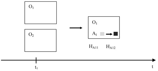
Figure 17.
Changes monitoring.
- NULL_category
Previous section deals with the undefined value categorization present in the index structure. It is modeled by the memory structure, to which individual segments of the index point. During the data retrieval, these values can be robustly obtained from the defined index. The NULL value itself does not have specific meaning and origin expression, therefore in the NULL_category can clause, you can specify the undefined value representation and categorization. You can enable or disable managing individual undefined value types in the result set by calling NULL_category clause parametrized by the name of the category, to which the index segment points. Note, that the name of the NULL_category is present in the null_representation data dictionary.
Syntax extension and clauses availability in a complex manner is the following:
| [CREATE TABLE table_name AS] |
| SELECT [ALL|DISTINCT|UNIQUE] |
| {*|attribute_name| function_name[(parameters)]} [,...] |
| FROM table_name [table_alias] [,...] |
| [WHERE condition_definition] |
| [EVENT_DEFINITION] |
| [SPATIAL_POSITIONS] |
| [TRANSACTION_RELIABILITY] |
| [MODEL_REFLECTION] |
| [CONSISTENCY_MODEL] |
| [EPSILON_DEFINITION] |
| [MONITORED_DATA_SET] |
| [GROUP BY column_list [function_list]] |
| [HAVING agg_function_conditions] |
| [TYPE_OF_GRANULARITY] |
| [NULL_CATEGORY] |
| [ORDER BY column_list [function_list,ASC|DESC] [,...]] |
6. Performance Evaluation
Performance characteristics have been obtained by using the Oracle 19c database system based on the relational platform. For the evaluation, a table monitoring 100 drivers was used, each row was delimited by the composite primary key—identification of the driver (driver_id) and spatio-temporal spheres (location_def, time_def). In the first phase, just data based on the smartphone sensors were used (5 sensors we used monitoring speed of the vehicle, eye-blinking, concentration, noise, and the number of people in the car). Data (5 sensors (s)) were obtained three times per minute (f) for 100 drivers (d) during three hours a day (t) (covering the transport to the office and back + going to the standard daily shops) monitored during one month—twenty working days (m). Thus, the total data amount in the table was (value of the t is expressed in minutes):
s ∗ f ∗ d ∗ t ∗ m = 5 ∗ 3 ∗ 100 ∗ 180 ∗ 20 = 5,400,000 data rows.
The total amount of the data in the table was 5.4 million. The main index was defined just for the driver and time-positional data definition, 10% of rows were delimited by at least partial undefinition (three categories were used for the undefinition). No other indexes were developed, therefore this main index was used for the Flower index approach as the Master index.
Experiment results were provided using Oracle Database 19c Enterprise Edition Release 19.3.0.0.0—64bit Production. Parameters of the used computer are:
- Processor: Intel Xeon E5620; 2.4 GHz (8 cores),
- Operation memory: 48 GB DDR 1333 MHz
- Disk storage capacity: 1000 GB (SSD).
To evaluate the performance, two approaches were used as the referencing. Model TAF does not deal with undefined values in the index definition, thus sequential scanning is necessary to be executed during the data retrieval. The second referential model can be named Model DEF, by which undefined values are transformed into the default values in the preprocessing layer outside the database. Thus, it is always ensured, that real data are present in the database, undefined values are modeled by using default value transformation. As evident from the results, it has additional demands on the disc storage. Data evaluation is more complicated, as well, whereas the default value has to be replaced during the result set composition and transport to the client.
A computational study dealing with the performance reflects processing costs delimited by the time demand aspect.
- Experiment 1—temporal architecture
As stated, the environment deals with data 5 sensors providing data for 100 drivers during three hours. In this evaluation experiment, 2 sensors were time-synchronized. In case of any Update operation, the random number of sensor values is changed, ranging from 2 to 4. This part deals with the temporal architecture with an emphasis on the processed granularity. Model Model_obj is delimited by the object architecture capturing the whole sensor image occurring during any Update statement. Model_column manages just separate sensors regardless of the synchronization of the 2 sensors. As evident, in this case, each changed attribute forces the system to load one extra row into the temporal layer. Model_group benefits from the synchronization group, which is defined and maintained automatically, based on the structure of the changes. If the group is changed, instead of managing individual sensors separately, data_val definition is used consisting of 2 physical sensor data, however, only one row for the whole group was inserted into the main temporal level. As evident, it proposes significant benefit during the Insert or Update statements, as well as during the data retrieval, whereas the result set should contain only actually changed values. Finally, model Model_group_ext is evaluated, which is based on synchronization based on the temporal data, as well as the positional data. In our case, we divide GPS data into 8 regions characterizing the map of our country. Note, that 10% of data portions are undefined, categorized into the 3 types randomly. Temporal, as well as spatial positions, can be undefined, thus such data are not indexed, by default.
Figure 18 shows the results of dealing with the data structure. To cover the complexity and reflection of the architecture, individual results are expressed in percentage. Based on the reached results, the most demanding architecture from the database structure point of view is the object architecture, which consists of several duplicates, if the attribute value is not changed. Therefore, we propose an additional model called Model_obj_imp, which does not store the original values multiple times, just the undefined value is used to handle it. In that case, the NULL categorization is extended by one element expressing data change. The limitation is just the necessity to evaluate the direct predecessor of the state to identify real change, which is not, however, size demanding. Column level architecture uses a preprocessing layer dividing the state into individual attributes. In that case, processing size demands are lowered to 46%. Attributes, which are not changed, are not stored in the new state, at all. Processing uses attribute granularity. Group solution separates individual attributes into the synchronization group, which is managed always as one module defined by the data_val value. Thanks to that, the number of requests to the temporal table is lowered. The total size demands are lowered to the value 38. In comparison with Model_obj, it reflects improvement using 62%. Comparing to the column architecture, it provides an 8% benefit in size demands. Model_group is based on temporality. Extending the model by the spatial positions is introduced in the model Model_group_ext. Individual data are categorized into 8 regions, which can be managed separately. In that case, processing demands in terms of the size are lowered to the value 34%, lowering the demands from 38 to 34% dealing with the group architecture. The benefit is based on the spatio-temporal categorization, thus the data can be obtained from the spatial, as well as temporal perspective. If internal partitioning is used, demands are almost the same, however, data retrieval is more straightforward, processing itself can be parallelized done on the internal partitions. Figure 18 shows the size demands.
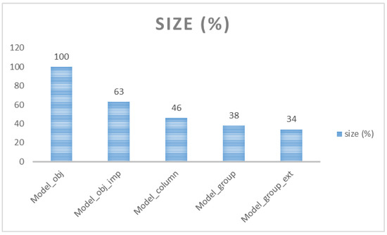
Figure 18.
Size demands.
- Experiment 2—data retrieval
Data retrieval process demands are based on the identification of the real change of the values. Thus, the most demanding architecture is Model_obj, in which individual rows must be sorted and compared to identify the change. If the data precision is not defined correctly, multiple phantoms can be present, which do not cover the changes, or vice versa, data values are considered as changed, which is not, however, true. Therefore, the reliability aspect is significantly inevitable in that solution. Column level architecture is optimal from the change identification requirement. Individual states are composed of the temporal layer directly. Group architecture is optimal regarding storage capacity. During data retrieval (changes monitoring), each group must be expanded into the individual column list, which requires additional 4% demands in comparison with column architecture. A slight benefit can be obtained by using spatio-temporality dealing with two layers grouping data separately. Thanks to that, the processing itself can be divided into the defined ranges formed by internal partitioning. Processing time demands are 40%. In comparison with object architecture, it lowers the demands using 60%, reflecting temporal group definition and spatio-temporal determination, it lowers the demands using 2%. Figure 19 shows the results in the graphical form.
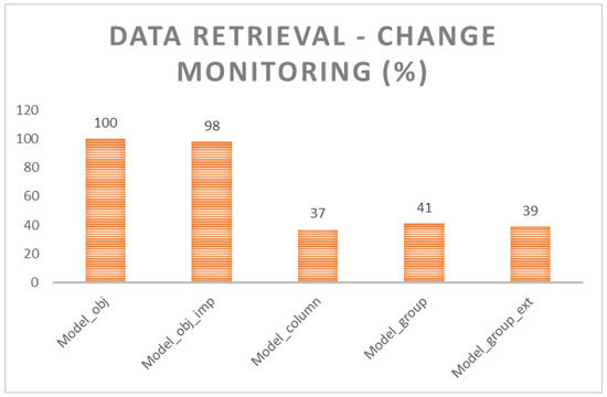
Figure 19.
Data retrieval (change monitoring).
Different order of efficiency is obtained, if the whole data image should be provided, regardless of the changes themselves. During the defined time frame or spatial regions, respectively, the whole data image should be part of the result set. In object-level architecture, the whole data image is present there, so it can be directly provided. Thus, from the size demands, requirements are significantly high, however, when dealing with the whole data image, particular data are directly in the database with no necessity for state composition and calculation. On the other hand, there is a relevant demand for the data loading from the database into the instance memory Buffer cache. Figure 20 shows the results. Reference model is Model_obj (100%). Improved model using object architecture dealing with the real change identification brings additional demands ranging 2%. The reason is based on the transformation necessary to the original form during the retrieval. It requires 10%, however, the demands are lowered using 8%, whereas the size of the structure is less, thus the number of blocks to be loaded is smaller. Attribute-oriented architecture, in comparison with object architecture, requires an additional 33%. The processing itself can be divided into two parts—object state composition from the individual attribute set—41% lowered by the block loading necessity—8%. Similar solutions are obtained by the group architecture, as well, additional necessity to decompose group is identified. Based on the results, it requires an additional 4 or 5%, respectively, in comparison with column granularity. Figure 20 shows the results.
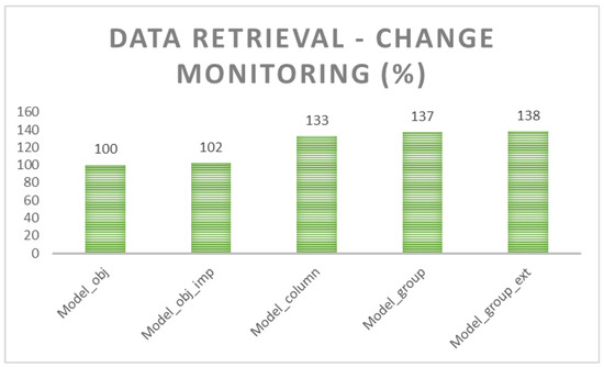
Figure 20.
Data retrieval (change monitoring).
- Experiment 3—adding new states
In conventional systems, individual changes are defined by the Update statement replacing the original state with the newer one. The new object is created by invoking the Insert statement. In a spatial environment, each object is delimited by the temporal scheme expressing validity, respectively of the period of occurrence. Thus, any change is physically modeled by the Insert statement, either in the case of adding a new state or the whole object definition, as well. This experiment aims to evaluate the demands of adding a new state into the database in terms of processing time. As defined, 5.4 million rows are present in the database after the operation by using various granularity levels. We compare the processing time to load the whole data set into the database with emphasis on the real change identification for the column level or synchronization detection used in group-level granularity. Each change is delimited by the separate transaction, data are logged and afterward stored in the database. No temporal consistency and model management is done, at all. Reference model is Model_obj (100%). If the same values are not stored physically, just the specific NULL category pointer is used, demands are 99% (Model_obj_imp). Physically, it requires additional demands in 7%, which is, however, lowered by the fewer size demands, whereas physically, the only pointer is used. By using column architecture, only real change is stored. In comparison with object architecture, a new row into the temporal layer is added only in the case of the real change. Object-level structure stores data values for each attribute. Column level architecture Insert statement demands are 64% in comparison with object architecture. When dealing with group management, demands can be lowered, slightly. Processing time value of the group architecture dealing with only time representation reflects 58%, spatial categorization into the regions 60%. It is the result of another processing layer and region management segmentation. Figure 21 shows the results.
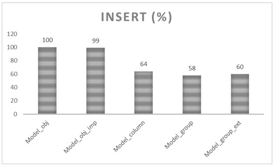
Figure 21.
Data loading (Insert statement).
- Experiment 4—LAR, TLAR, ETLAR
In the previous experiment, only a standardized conventional LAR approach was used. Particular data were logged and stored in the database based on the defined granularity. Data integrity, collisions, and model reflection were, however, not taken into emphasis. This section deals with the proposed rules TLAR and ETLAR referencing the current state of the art solution defined by the Log Ahead Rule. TLAR extends the definition by identifying and solving transaction rules to limit the overlapping states on the one object. Several rules can be applied to ensure consistency—a new valid state is either refused (REFUSE) or the validity of either the existing or new state is shortened (SHORTEN) or the states are moved in time (REPOSITION). This experiment evaluates the processing time demands or those three rules. The used architecture is group-oriented used as a reference model (100%). 20% of states to be added cause anomaly collision. If the REFUSE rule is used, the demands are even lowered, whereas the data themselves are not loaded into the database, only information about the temporal attempt to insert a new state is noticed. The SHORTEN rule is the most demanding, whereas the data themselves must be changed by locating existing and newly added rows. If the existing row must be updated, the total demands have risen to 109% reflecting the 9% of additional demands in comparison with the reference model LAR. In the newly inserted row, validity is changed, additional demands are 5%, whereas either begin point or end point of the validity must be shifted (shortened). In this criterion, defined states do not force the system to refuse the state completely, so there is only partial overlapping of the existing state. In this case, based on the data, we assume, that only one valid state is influenced. If multiple states are necessary to be evaluated, in general, approximately 0.5% for each state is added to the processing time demands. REPOSITION criterion influences the time positions, validity interval in terms of its length is not influenced, at all, however, the period placement into the timeline is enhanced. In that case, 3% of additional processing time costs are present, as the result of the placement identification. Similarly, we assume, that there is a collision with one state only. The ETLAR rule extends the previously defined criteria by covering the model relevance. If the particular model is not present, the newly added state can be either refused (ETLAR strict) or the current data model can be reflected (ETLAR ignore). Management of the integrity of the time-evolving data model and constraints require an additional 4% of the processing time, however, the consistency can be always ensured, no integrity constraint lacks can be later detected. In the case of using the Ignore option, additional demands are 6%, whereas the new state is always inserted with the specific flag regarding the particular model availability. Note, that by using the Strict rule, the state to be loaded can be refused completely, forcing the system not to insert data into the database, which has namely benefits in the disc operations.
Figure 22 shows the reached results for the 100 driver data sensor evaluation.
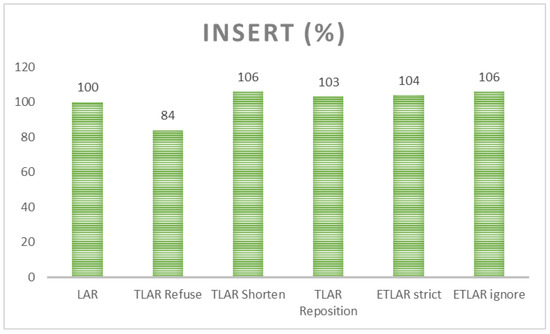
Figure 22.
Insert—Log Ahead Rule (LAR), Temporal Log Ahead Rule (TLAR), Extended Temporal Log Ahead Rule (ETLAR).
- Experiment 5—null management
Undefined value management forms a crucial aspect limiting the performance and evaluation process. As stated, NULL values are not part of the B+index structure. Furthermore, it does not have a specific meaning. We cannot state in the temporal sphere, whether such event will be in the future or not, even whether such events have not occurred yet, particular states cannot be sorted, mathematically treated, and evaluated by the origin of a given undefined value. Therefore, this experiment covers the performance definition protected by undefined value management. The core architecture uses the group granularity evaluated in experiment 1 (Model_group). The environment solution deals with the three models. The reference model (Model_no_null) is delimited by the pure spatio-temporal architecture, which cannot cover undefined values in the index structure, at all. Model_null covers only undefined values in one category with no origin reflection. It does not have any storage demands, whereas such NULL values are not treated physically. By adding an external module associated with the index root node, NULL values can be placed in the structure and located by the index itself. The demands, in comparison with Model_no_null, are lowered to the value 72%, as the result of the undefined value accessibility by the index by replacing Table Access scanning necessity by the index approach managing data range. Thus, it uses the Index Range Scan method or Unique Scan, respectively, if the condition is based on a unique value set. Model_null_cat reflects the memory structure NULL_representation as the pointer layer delimiting the meaning and origin of the undefined values. In this case, 3 categories for treating NULLs are used, however, based on the evaluation, it can be stated, that the number of categories has minimal impact on the performance. The difference is just the pointer destination, however, the size and principle reflection remains still the same. When dealing with the NULL categorization, reached performance results are 73% in comparison with Model_no_null. Comparing index structures dealing with undefined values inside the system (Model_null and Model_null_cat), there is only a slight performance difference, which is, however, fulfilled by obtaining more complex information regarding the undefined value origin and reliability of the data. If the Model_null is referential (treated as 100%), then the Model_null_cat requires additional power ranging 1.38%. Figure 23 shows the results reflecting group granularity with various NULL management definition principles.
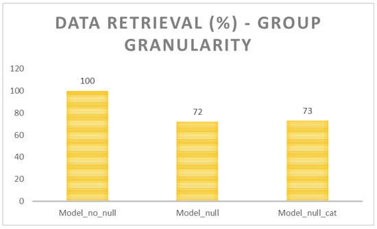
Figure 23.
Data retrieval—NULL management layer.
- Experiment 6—whole solution architecture
A specific feature of the spatio-temporal system is just the requirement for extremely fast and efficient processing. Input data are often obtained from sensory networks or systems themselves, where the emphasis is on the almost immediate processing with no delays. Data retrieval efficiency covered by the speed is a critical factor as the states of objects change dynamically. Experiment 6 focuses on the efficiency of obtaining data from the database, comprehensively monitors the process of identification and localization of individual object state records. It uses the modules defined in this paper, the benefits of which are evaluated in the retrieval process depending on their presence in the system. The first used module reflects the Epsilon definition covering just relevant data changes. We used the 0.1% threshold for shifting data into the database or reuse the original value, respectively. In principle, data are provided in the defined time frames, however, the input does not need to be stored in the database, if the significant change is not detected. In that case, the amount of data in the database is lowered with no impact on the data quality. Each data value is then extended by the 0.1% precision interval. The second module presence reference the Master indexing, which removes the impact of the whole table scanning, if no suitable index is used. In that case, block values are extracted from any suitable B+tree by scanning the leaf layer of the index. Master index selection used in this experiment was dynamic meaning, that the optimizer autonomously selects the best suitable index with minimal estimated costs reflected by the memory loading (I/O operations from the database), whole size, and costs of the scanning. Note, that the index must cover all data rows, otherwise it cannot be marked as Master. The third accessible module reflects NULL management directly in the index set. Thanks to the presence of this module, any index can be selected as Master. In this case, the existing index set does not been to be enhanced, but if the condition is based on the undefined or untrusted value, the existing index can be used, as well. By using the NULL management module, many times, the original index can be directly used with no necessity to block identification (BLOCKID) extraction. The fourth module uses range spatial partitioning using the defined regions. It follows the temporal data partitioning, as well, thus the data image valid at the defined timepoint or interval is placed in the same data partition, thus the evaluation is easier and significantly less demanding, whereas the number of searched data is minimized. Moreover, if the data interval is spread across multiple partitions, the background process launches more workers to process the data in parallel. Afterward, the result set is created by the unification of the sets (UNION ALL operation). The fifth module expresses the autoindexing option, by which the existing index set is dynamically analyzed, new indexes are created and removed autonomously with regards to the whole performance of the current states. By using the Master indexing module, peaks created by the autoindexing can be flattened. The reason is, that the autoindexing is just the reactive module based on the changed query types. Moreover, the index must be built to be usable, which demands additional processing time and system sources. If the system is so dynamic with really various query types evolving rapidly over the time, the autoindexing module does not even provide benefits, whereas the costs of the index set handling can be higher in comparison with the total contribution. In this case, based on the number of uses of the given index (provided by the statistics), the system evaluates that the benefit of the autoindexing module is minimal and is automatically deallocated. At the same time, however, the system is monitored and, if the benefits exceed the costs, it switches on automatically. The last module is post-indexing, which extracts the index balancing operation into a separate transaction. Thanks to that, a particular Insert operation can be ended sooner by reaching the transaction Commit earlier. Thus, the data are produced for the environment by lowering the processing delays. Figure 24 shows the architecture with the relevance of the individual modules. The experiment uses the assumption, that all preceding modules are present in the system. Thus, by introducing NULL management, Epsilon, and Master index modules are already there. Note, that index set consists of the spatial and temporal reflection only. There is no additional index present unless created by the autoindexing.
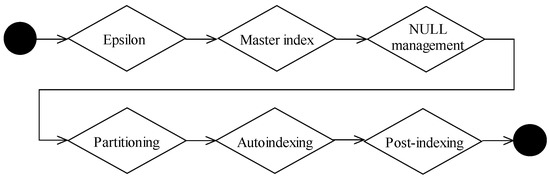
Figure 24.
Whole system modularization.
The reference model does not use any already defined modules (reference 100%). Reflecting the sensor-based data about the drivers defined in [28] reflecting principles covered in [40,41,42], Epsilon definition lowers the processing time demands to 87%. Evaluation is done in the preprocessing layer of the database system, individual background processes are contacted only if it reflects the relevant change. Master index extension requires only 81%. Its benefit is based on the fragmentation, which is present at 10%, of which 3% of the blocks are empty. Migrated row problem is not present, whereas there are not physical updates. NULL management module significantly improves the performance, first of all, the index can be always used, whereas pointers to the whole relevant data are there, secondly, the Master index portfolio set can be extended, as well, any index can be marked as Master. NULL module extension limits the demands to the value of 69% if there is no specific categorization of the NULL values. If the 3-type categorization is present, the demands are 73%. One way or another, there is always a 10% demand drop. Spatio-temporal partitioning, as stated, allows the process of data in parallel. Spatiality is covered by 8 regions. It requires 55%, which is mostly caused by parallel processing followed by the result set unification. Autoindexing module covers only 4% benefit in comparison with the already defined modules. Based on the analysis, there is no significant space for improvement. Master index and NULL management modules ensure, that the whole table scanning, block by block, is not executed at all. Vice versa, adding a new index dynamically benefits only if the query type set is relatively static, otherwise, the whole module is disabled, it cannot predict the future queries to handle indexes. The main advantage of the post-indexing is the extraction of the B+tree index balancing directly during the main processing. Thus, when dealing with data changes, the solution benefits. Vice versa, during the data retrieval process, it cannot be ensured, that all changes are already applied to the indexes, thus the evaluation must be two-phase—the index itself is evaluated and scanned to find relevant data directly or ROWID or BLOCKID, respectively. As stated, it does not need to cover all changed data, therefore the Notice list must be checked and relevant changes extracted. The total demands are 54% if the autoindexing is enabled. If it is disabled, it requires 57%. Figure 25 shows the results in the graphical form.
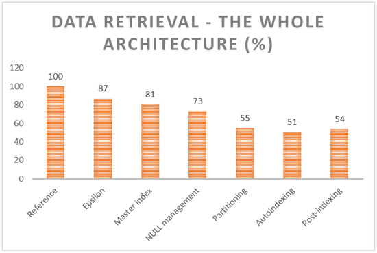
Figure 25.
Whole system modularization—data retrieval performance.
- Summary
Data retrieval is a complex staged process, each stage influences the performance. In principle, any incorrect decision done on any layer cannot be corrected later. The first level covers architecture. In this paper, we deal with sensor data management operated to monitor driver activity, over time forming temporal architecture. Based on the defined environment and 5.4 million rows, it is evident, that the data changes are not always present for each attribute synchronously. If the heterogeneity of the specification is present, the problem can be even deeper, whereas some data portions do not change their values at all forming the code list principles. Another problem is correlated with the data, which do not need to be monitored over time. Thus, in any environment, where such prerequisites are present, the proposed solution is relevant. Based on the results, the size of the whole structure can be reduced up to 66% for the group extension architecture. The data retrieval process can significantly benefit, as well, whereas the change identification is directly evident for the attribute (column) or group granularity. Reflecting the performance and environment, demands are lowered using 63% for attribute and 61% for the group, which is reflected by the group decomposition necessity.
Undefined values form another complex problem, whereas they are not located in the index structures. For data retrieval, therefore, sequential data block scanning is necessary to be done. By using proposed NULL modules and categorization, processing demands in terms of time can be lowered up to 27% or 28%, respectively. Finally, complex architecture is evaluated covering all the proposed segments summarized in Figure 24. The usage of the proposed solutions can be found in almost any environment necessary to monitor sensor data over time. In the industry environment, the individual manufacturing process needs to be monitored by the sensors, which produce relevant data with various granularity and precision. If the measured data value is provided with delay and the sensor is broken or the communication channel fails, even temporarily, undefined values are produced, which must be handled with care. The proposed solution can be, similarly, used for traffic monitoring, for the positional data processing of the vehicles, or flight efficiency and position monitoring. Area of patient monitoring can benefit by using the proposed architecture, as well. In this paper, moreover, data retrieval extension clauses are proposed, by which the user experience benefits. The process of the data to be obtained is significantly simplified. The following paragraph shows the benefit of the proposed solutions. The first example deals with the Epsilon management, only rows, that express the change above 1% that will be part of the result set. In the existing syntax, it is necessary to use the flowing window frame to obtain the previous value of the sensor particular for the object. Note, that it cannot be done directly, thus the nested Select statement needs to be used. Moreover, if the window does not reflect only the direct predecessor, a more complex solution must be specified. The second code shows the usage of the Epsilon clause definition, which simplifies the specification, however, the performance is the same:
| Select object, BD, value |
| From |
| (Select object, BD, value, |
| lag(value, 1<=offset, null<=default) |
| over(partition by object order by BD) as predecessor |
| From data_tab) |
| Where abs(value, predecessor)>1; |
By using proposed Select statement definition, the same results are obtained:
| Select object, BD, value |
| From data_tab |
| Where Epsilon_definition(value, 1); |
The following code shows the statement to monitor the vehicle in the Slovakia region during the year 2020 by monitoring delays. Whereas several new road segments were opened, as well as some existing are closed due to the reconstruction, current Model_reflection is used. Monitoring is specified by the Monitored_data_set clause, namely, driver and road properties are monitored.
| Select driver_data, road_parameters |
| From data_tab |
| Where Defined_interval(year(2020)) |
| And Epsilon_definition(road_parameters, 1%) |
| And Monitored_data_set(road_parameters) |
| And Model_reflection(AS-IS) |
| And Type_of_granularity(group(driver) as driver_data, |
| group(road) as road_parameters); |
Note, that without such clauses, really complicated script should be written.
Finally, there is an definition of driver route planning, thus the AS_WILL_BE model is reflected. Note, that without such clause, multiple tables across models should be necessary to be joined together, forming the complex environment. The planned journey is for 1 June 2021, reflecting the current environment pointing to the undefined limitations—traffic jams, closures, and fog.
| Select driver_data, road_parameters |
| From data_tab |
| Where Defined_interval(1-june 2021) |
| And Epsilon_definition(road_parameters, 1%) |
| And Monitored_data_set(road_parameters) |
| And Model_reflection(AS-WILL-BE) |
| And Type_of_granularity(group(driver) as driver_data, |
| group(road) as road_parameters) |
| And NULL_category(traffic_jams, closures, fog); |
7. Conclusions and Future Work
The core element influencing the quality and usability of any information system is associated with the data, their correctness, reliability, and accessibility in an effective manner. Currently, it is inevitable to store not only current valid data, but the emphasis should be taken to the whole evolution over time. The temporal database approach forms a robust solution, treating the time delimited states of the objects. In this paper, we summarize existing approaches dealing with the data granularity—the object-level temporal system extending the definition by the validity time frame. Column level architecture deals with data monitoring using the attribute level. The interlayer between object and column architecture is covered by the synchronization groups. In this paper, we propose the extension of the group solution in a spatial manner categorizing data into the regions.
When dealing with the data, whole integrity aspects must be cared for. Data models and integrity rules can evolve over time, as well. Therefore, we propose an extended conventional Log Ahead Rule dealing with either data state collisions in a temporal manner (TLAR), whereas each object can be defined just by one valid state anytime or extended version (ETLAR) covering temporal collisions, as well as data model relevance. Thanks to that, complex integrity can be ensured. Such rules are performance evaluated, as well.
Undefined values originating from various circumstances can be present in the input data stream, as well. If the untrusted ad-hoc network is present, the problem can be even deeper. In this paper, we discuss the costs and benefits of undefined values. NULL representation is not physically placed in the database, thus it does not additional store demands. On the other hand, dealing with NULL proposes a significant performance problem by locating data. Generally, data are obtained by the indexes, which cover logarithmic complexity instead of linear by using the Table Access Full method scanning block by block sequentially. The most often index used in the relational platform is B+tree, which cannot, however, cover undefined values inside it. As the consequence, when dealing with undefined values, which are most likely present in the systems, the whole block set associated with the table must be scanned, resulting in poor performance. Note, that the data fragmentation can be present there, forcing the system to load the particular block with no relevant data into the memory for the evaluation. In this paper, a complex solution for managing undefined values directly inside the index is present. It is based on an additional structure connected to the root index element. NULL values can have several representations and meanings, therefore we propose undefined data value type categorization. In this paper, we propose the NULL_represenation data dictionary object and memory pointer layer interconnected with the index module. Thanks to that, the index can be always used, whereas all references are present there.
The benefit of this paper is covered in Section 5, as well, covering the data retrieval process. No additional clauses dealing with the spatio-temporality are present, therefore we propose transformation clauses Event_definitions, Spatial_positions, Transaction_reliability, Model_reflection, Consistency_model, Epsilon_definition, and Monitored_data set operated in the Where condition of the Select statement. Type_of_granualarity and Null_category clause domains can be present in the Having clause, by which the output format can be treated. Evaluation of the proposed methods is divided into multiple experiments—impact granularity, transaction rules definition, indexing managing NULLs. The whole architecture is covered by experiment 6, which deals with the various modules, which are evaluated to emphasize the performance impacts. Namely, we are dealing with the Epsilon definition, Master indexing, NULL management, partitioning, autoindexing, and post-indexing, which extracts the index balancing method into the separate transaction supervised by the Index Balancer background process operated on the Notice list by applying individual changes into the index itself. Whereas multiple references to the index can be grouped and operated in a single balancing method, performance benefits. Whereas the changes to the index set are applied almost immediately, it does not have a significant impact on the data retrieval performance. Moreover, index and Notice lists can be treated in parallel followed by the unification.
In the future, we would like to extend the techniques to the data distributed environment, treating various index block size structures and tablespace locations. Data balancing over the networks, as well as data fragmentation and replication techniques in the spatio-temporal environment, will be covered by future research, as well.
Author Contributions
Conceptualization, M.K. and K.M.; methodology, M.K.; software, E.K.; validation, M.K., E.K. and K.M.; formal analysis, M.K. and E.K.; investigation, M.K. and K.M.; resources, E.K.; data curation, E.K.; writing—original draft preparation, M.K.; writing—review and editing, M.K.; visualization, K.M.; supervision, E.K.; project administration, M.K., E.K. and K.M.; funding acquisition, E.K. All authors have read and agreed to the published version of the manuscript.
Funding
This research received no external funding.
Institutional Review Board Statement
Not applicable.
Informed Consent Statement
Not applicable.
Data Availability Statement
Not applicable.
Acknowledgments
This publication is the result of the project implementation: Centre of excellence for systems and services of intelligent transport II. ITMS 26220120050 supported by the Research & Development Operational Programme funded by the ERDF. The work is also supported by the project VEGA 1/0089/19 Data analysis methods and decisions support tools for service systems supporting electric vehicles and by the Grant System of University of Zilina No. 9/2020.
Conflicts of Interest
The authors declare no conflict of interest.
References
- Laszewski, T.; Arora, K.; Farr, E.; Zonooz, P. Cloud Native Architectures: Design High-Availability and Cost-Effective Applications for the Cloud Kindle Edition; Packt: Birmingham, UK, 2018. [Google Scholar]
- Jakobczyk, M.T. Practical Oracle Cloud Infrastructure: Infrastructure as a Service, Autonomous Database, Managed Kubernetes, and Serverless; Apress: New York, NY, USA, 2020. [Google Scholar]
- Dey, D.; Barron, T.M.; Storey, V.C. A conceptual model for the logical design of temporal databases. Decis. Support Syst. 1995, 15, 305–321. [Google Scholar] [CrossRef]
- Kvet, M.; Salgova, V.; Kvet, M.; Matiasko, K. Master Index Access as a Data Tuple and Block Locator. In Proceedings of the Conference of Open Innovation Association, FRUCT, Helsinki, Finland, 6–8 November 2019. [Google Scholar]
- Bryla, B. Oracle Database 12c: The Complete Reference; McGraw-Hill Education: New York, NY, USA, 2013; ISBN 978-0071801751. [Google Scholar]
- Kyte, T.; Kuhn, D. Expert Oracle Database Architecture; Apress: New York, NY, USA, 2014. [Google Scholar]
- Gopalakrishnan, K.; Alapati, S. Oracle Database 12c Release 2 Real Application Clusters Handbook: Concepts, Administration, Tuning & Troubleshooting; McGraw-Hill Education: New York, NY, USA, 2018. [Google Scholar]
- Date, C.J. Database Design and Relational Theory: Normal Forms and All That Jazz; Apress: New York, NY, USA, 2019. [Google Scholar]
- Pornphol, P.; Chittayasothorn, S. Temporal database application in industrial human resource management. In Proceedings of the CIE 2014-44th International Conference on Computers and Industrial Engineering, Istanbul, Turkey, 14–16 October 2014. [Google Scholar]
- Johnston, T.; Weis, R. Managing Time in Relational Databases: How to Design, Update and Query Temporal Data; Morgan Kaufmann: Burlington, MA, USA, 2010. [Google Scholar]
- Ailamaki, A.; Johnson, R.; Pandis, I.; Tözün, P. Toward scalable transaction processing. In Proceedings of the VLDB Endowment, Trento, Italy, 26–30 August 2013. [Google Scholar]
- Unnikrishnan, K.; Pramod, K.V. On implementing temporal coalescing in temporal databases implemented on top of relational database systems. In Proceedings of the International Conference on Advances in Computing, Communication and Control, ICAC3’09, Mumbai, India, 23–24 January 2009. [Google Scholar]
- Park, J.-H. Low-cost image indexing for massive database. Multimed. Tools Appl. 2015, 74, 2237–2255. [Google Scholar] [CrossRef]
- Date, C.J. Time and Relational Theory: Temporal Databases in the Relational Model and SQL (The Morgan Kaufmann Series in Data Management Systems; Morgan Kaufmann: Burlington, MA, USA, 2014. [Google Scholar]
- Dhont, M.; Tsiporkova, E.; Boeva, V. Layered Integration Approach for Multi-view Analysis of Temporal Data, Advanced Analytics and Learning on Temporal Data. In Proceedings of the 5th ECML PKDD Workshop, AALTD 2020, Ghent, Belgium, 18 September 2020. [Google Scholar]
- Peng, T.; Sellami, S.; Boucelma, O. Trust Assessment on Streaming Data: A Real Time Predictive Approach, Advanced Analytics and Learning on Temporal Data. In Proceedings of the 5th ECML PKDD Workshop, AALTD 2020, Ghent, Belgium, 18 September 2020. [Google Scholar]
- Rabcan, J.; Rusnak, P.; Zaitseva, E.; Macekova, D.; Kvassay, M.; Sotakova, I. Analysis of Data Reliability based on Importance Analysis. In Proceedings of the International Conference on Information and Digital Technologies IDT, Zilina, Slovakia, 25–27 June 2019. [Google Scholar]
- Levashenko, V.; Lukyanchuk, I.; Zaitseva, E.; Kvassay, M.; Rabcan, J.; Rusnak, P. Development of Programmable Logic Array for Multiple-Valued Logic Functions. IEEE Trans. Comput. Aided Des. Integr. Circuits Syst. 2020, 39, 4854–4866. [Google Scholar] [CrossRef]
- Zaitseva, E.; Levashenko, V.; Rabcan, J.; Kvassay, M.; Rusnak, P. Reliability Evaluation of Multi-State System Based on Incompletely Specified Data and Structure Function. In Proceedings of the 2019 10th IEEE International Conference on Intelligent Data Acquisition and Advanced Computing Systems: Technology and Applications, IDAACS, Metz, France, 18–21 September 2019. [Google Scholar]
- Kvet, M. Solution Management for Current Temporal Aspect Using Tuple Versions. In Proceedings of the Conference of Open Innovation Association, FRUCT, Trento, Italy, 7–9 September 2020; No. 27. pp. 101–107. [Google Scholar]
- Lu, W.; Zhao, Z.; Wang, X.; Pan, A.; Du, X. A Lightweight and Efficient Temporal Database Management System in TDSQL. Proc. VLDB Endow. 2018, 12, 2035–2046. [Google Scholar] [CrossRef]
- Yen, I.-L.; Chen, I.-R.; Chen, B. Real-time atomic transaction processing using multi-invariant data structure. In Proceedings of the 4th IEEE International Symposium on High-Assurance Systems Engineering, Washington, DC, USA, 17–19 November 1999; pp. 161–168. [Google Scholar]
- Kvet, M.; Krsak, E.; Matiasko, K. Locating and accessing large datasets using Flower Index Approach. Concurr. Comput. Pract. Exp. 2020, 32, e5209. [Google Scholar] [CrossRef]
- Dunaieva, I.; Barbotkina, E.; Vecherkov, V.; Nikonorov, A.; Akimov, L. Spatial and temporal databases for decision making and forecasting. In Advances in Intelligent Systems and Computing 1259 AISC; Springer: Berlin/Heidelberg, Germany, 2021; pp. 198–205. [Google Scholar]
- Kvet, M.; Matiasko, K. Analysis of current trends in relational database indexing. In Proceedings of the 2020 International Conference on Smart Systems and Technologies (SST), Osijek, Croatia, 14–16 October 2020; IEEE: Piscataway, NJ, USA, 2020. [Google Scholar]
- Lewis, J. Cost-Based Oracle Fundamentals; Apress: New York, NY, USA, 2005. [Google Scholar]
- Sanchez, C.S.; Wieder, A.; Sottovia, P.; Bortoli, S.; Baumbach, J.; Axenie, C. GANNSTER: Graph-Augmented Neural Network Spatio-Temporal Reasoner for Traffic Forecasting, Advanced Analytics and Learning on Temporal Data. In Proceedings of the 5th ECML PKDD Workshop, AALTD 2020, Ghent, Belgium, 18 September 2020. [Google Scholar]
- Kvet, M.; Matiasko, K. Data Block and Tuple Identification Using Master Index. Sensors 2020, 20, 1848. [Google Scholar] [CrossRef] [PubMed]
- Pokorný, J.; Stantic, B. Big data processing and big analytics. In Emerging Technologies and Applications in Data Processing and Management; IGI Global: Hershey, PA, USA, 2019; pp. 285–315. [Google Scholar]
- Lew, M.S.; Huijsmans, D.P.; Denteneer, D. Optimal keys for image database indexing. In Lecture Notes in Computer Science; Springer: Berlin/Heidelberg, Germany, 1997. [Google Scholar]
- Lo, Y.-L.; Tan, C.-Y. A study on multi-attribute database indexing on cloud system. In Lecture Notes in Engineering and Computer Science; Springer: Berlin/Heidelberg, Germany, 2012. [Google Scholar]
- Chen, H.; Li, J. The research of embedded database hybrid indexing mechanism based on dynamic hashing. In Lecture Notes in Electrical Engineering; Springer: Berlin/Heidelberg, Germany, 2013. [Google Scholar]
- Radaideh, M.A. A distributed and parallel model for high-performance indexing of database content. Int. J. Comput. Appl. 2004, 26, 257–262. [Google Scholar]
- Kato, K. Persistently cached B-trees. IEEE Trans. Knowl. Data Eng. 2003, 15, 706–720. [Google Scholar] [CrossRef]
- On, S.T.; Hu, H.; Li, Y.; Xu, J. Flash-optimized B+-tree. J. Comput. Sci. Technol. 2010, 25, 509–522. [Google Scholar]
- Lilien, L.; Bhargava, B. Database Integrity Block Construct: Concepts and Design Issues. IEEE Trans. Softw. Eng. 1985, 11, 865–885. [Google Scholar] [CrossRef]
- Oracle Documentation-Autoindexing. Available online: https://blogs.oracle.com/oraclemagazine/autonomous-indexing (accessed on 1 December 2020).
- Nimkanjana, K.; Vanichayobon, S.; Wettayaprasit, W. Auto-Indexing Selection Technique in Databases under Space Usage Constraint Using FP-Growth and Dynamic Programming. In Proceedings of the 2008 International Conference on Computer and Electrical Engineering, Phuket, Thailand, 20–22 December 2008. [Google Scholar]
- Oracle Documentation–INTERVAL Data Type. Available online: https://docs.oracle.com/en/database/oracle/oracle-database/19/sqlrf/Data-Types.html#GUID-E405BBC7-DA9A-4DF2-9F22-E60CB9EC0705 (accessed on 1 December 2020).
- Ehlers, U.C.; Ryeng, E.O.; McCormack, E.; Khan, F.; Ehlers, S. Assessing the safety effects of cooperative intelligent transport systems: A bowtie analysis approach. Accid. Anal. Prev. 2017, 99, 125–141. [Google Scholar] [CrossRef]
- Levina, A.I.; Dubgorn, A.S.; Iliashenko, O.Y. Internet of things within the service architecture of intelligent transport systems. In Proceedings of the 2017 European Conference on Electrical Engineering and Computer Science, EECS, Bern, Switzerland, 17–19 November 2017. [Google Scholar]
- Wang, S.; Zhang, Z.; Wu, Z.; Liu, J.; Mo, C. Driver Drowsiness Analysis Based on Eyelid Feature. In Lecture Notes in Electrical Engineering; Springer: Berlin/Heidelberg, Germany, 2021. [Google Scholar]
Publisher’s Note: MDPI stays neutral with regard to jurisdictional claims in published maps and institutional affiliations. |
© 2021 by the authors. Licensee MDPI, Basel, Switzerland. This article is an open access article distributed under the terms and conditions of the Creative Commons Attribution (CC BY) license (http://creativecommons.org/licenses/by/4.0/).