
Estimation of the Noise Source Level of a Commercial Ship Using On-Board Pressure Sensors


Abstract
1. Introduction
2. Method and Validation
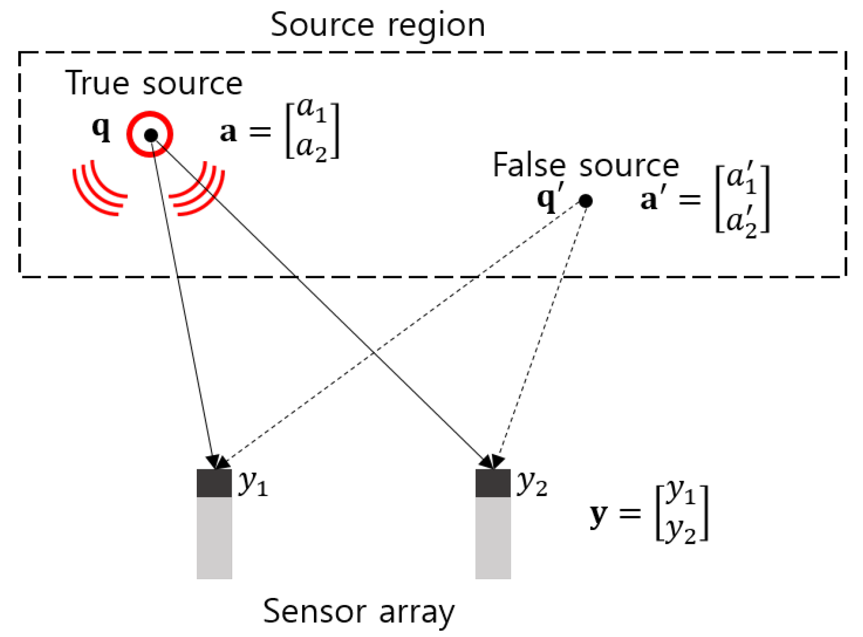
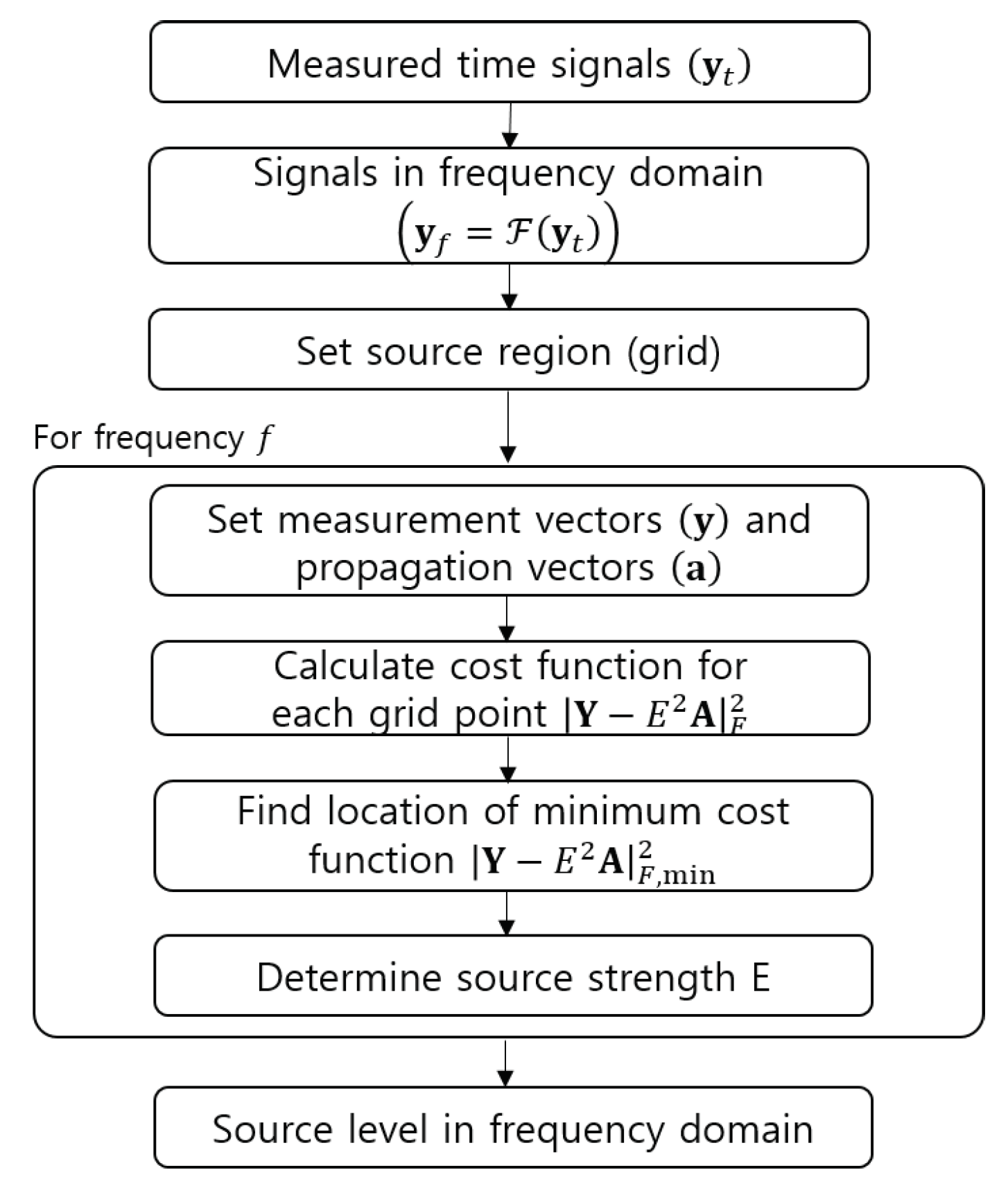
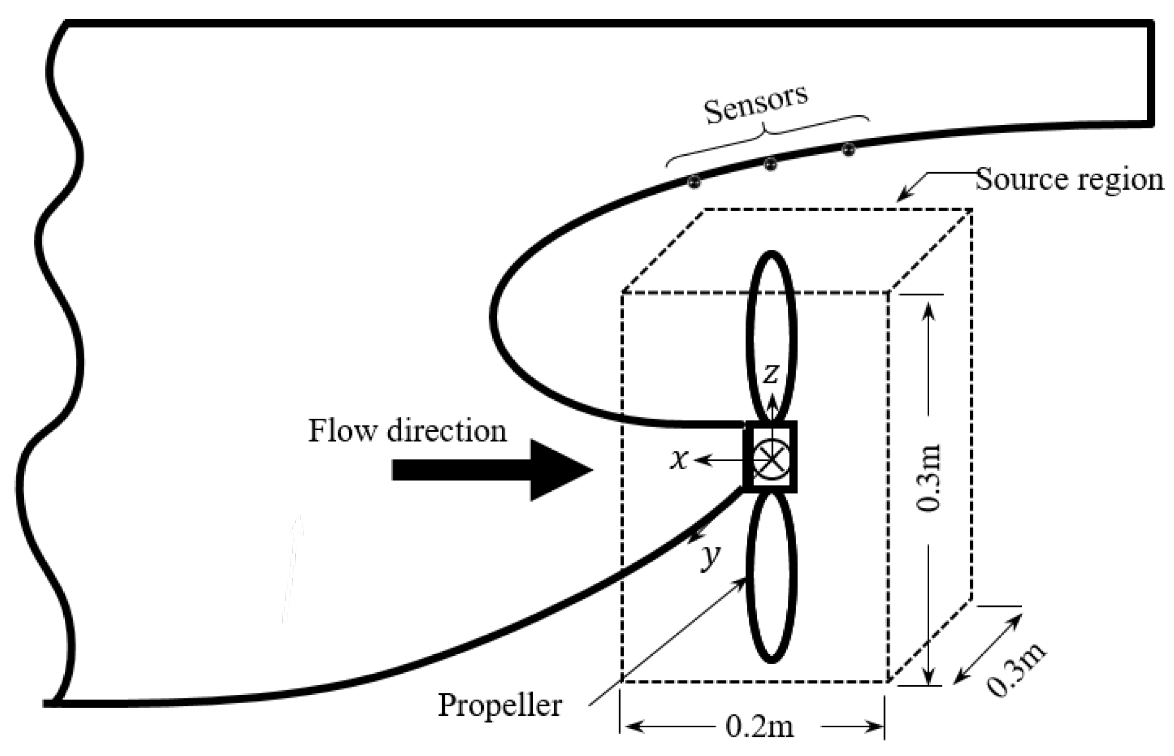
2.1. Methodology
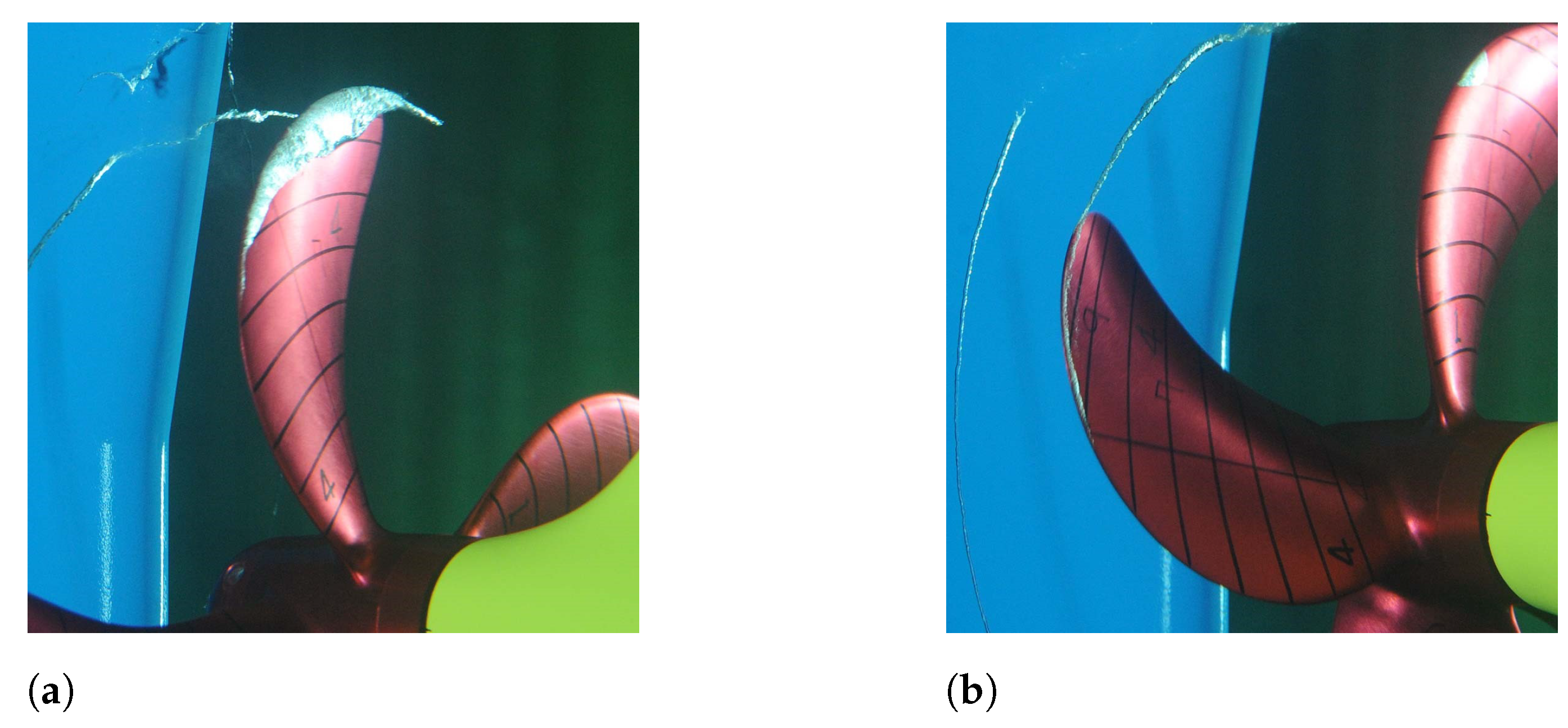
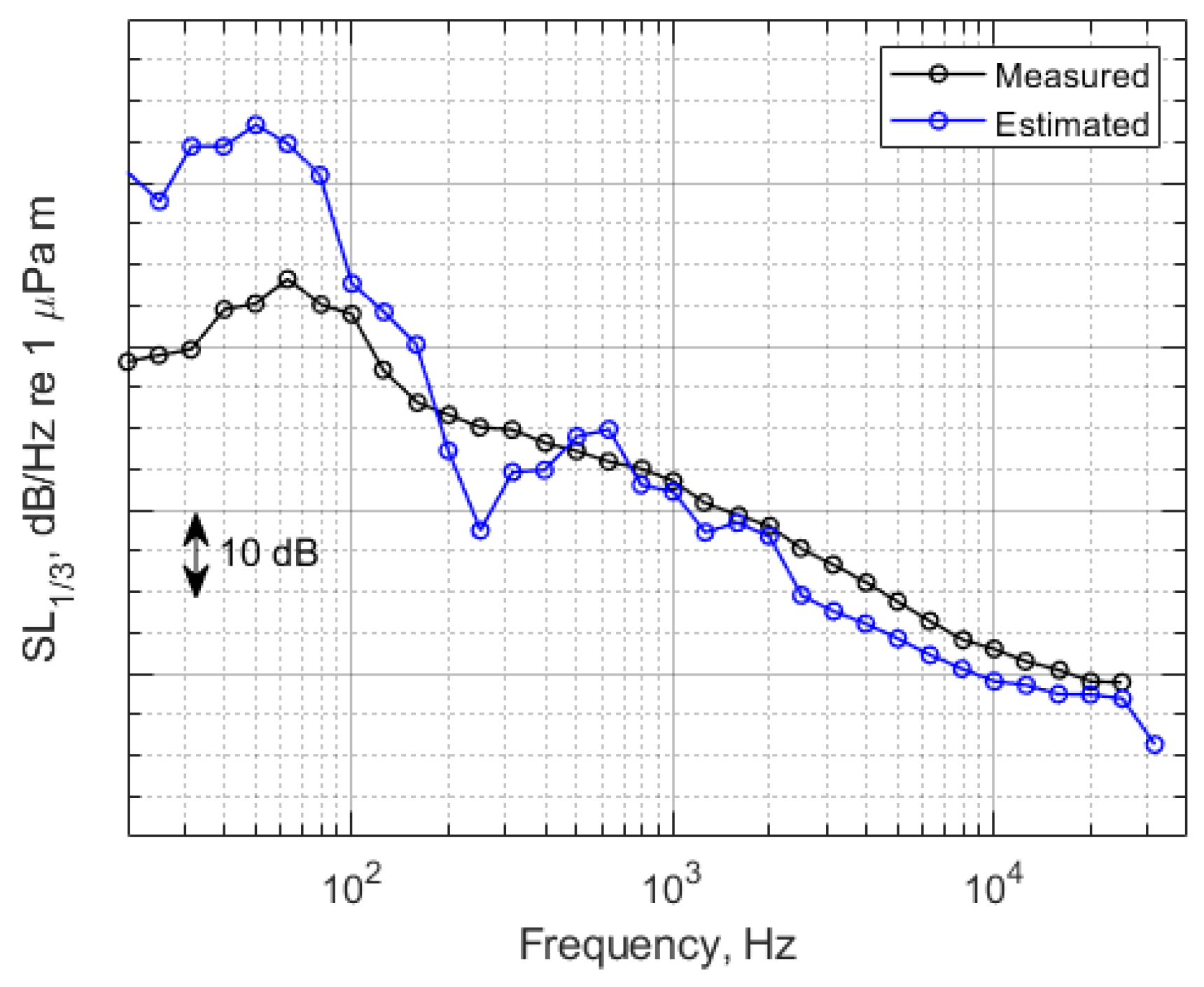
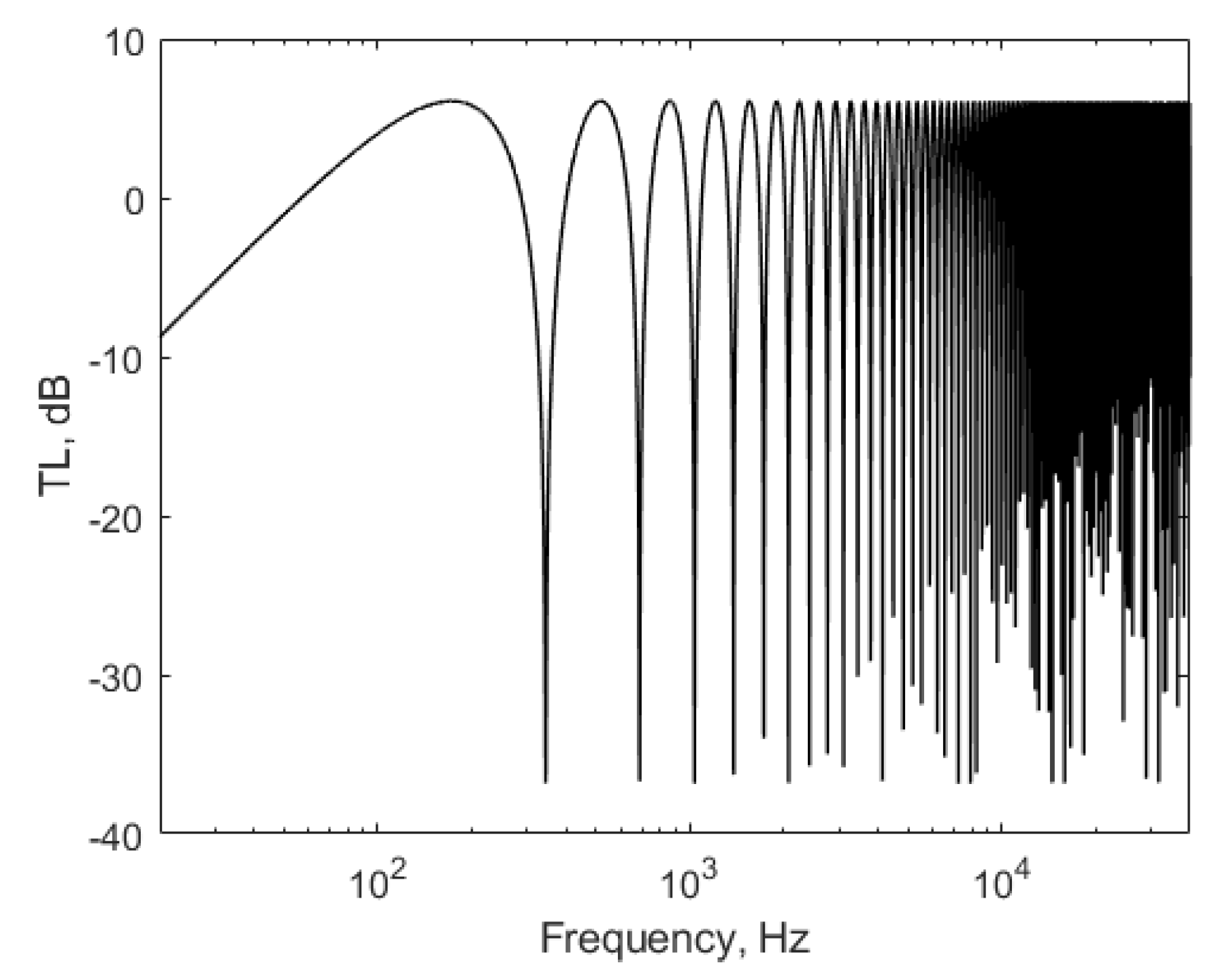
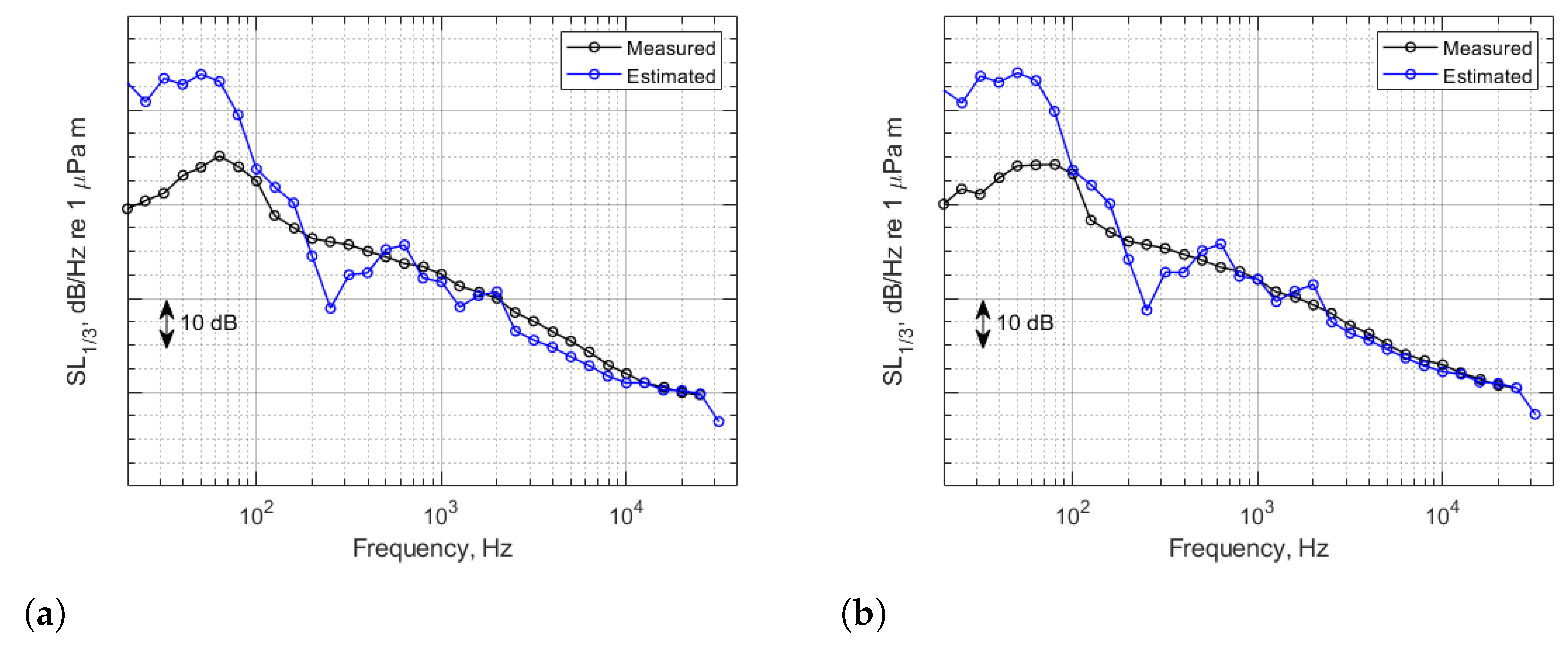
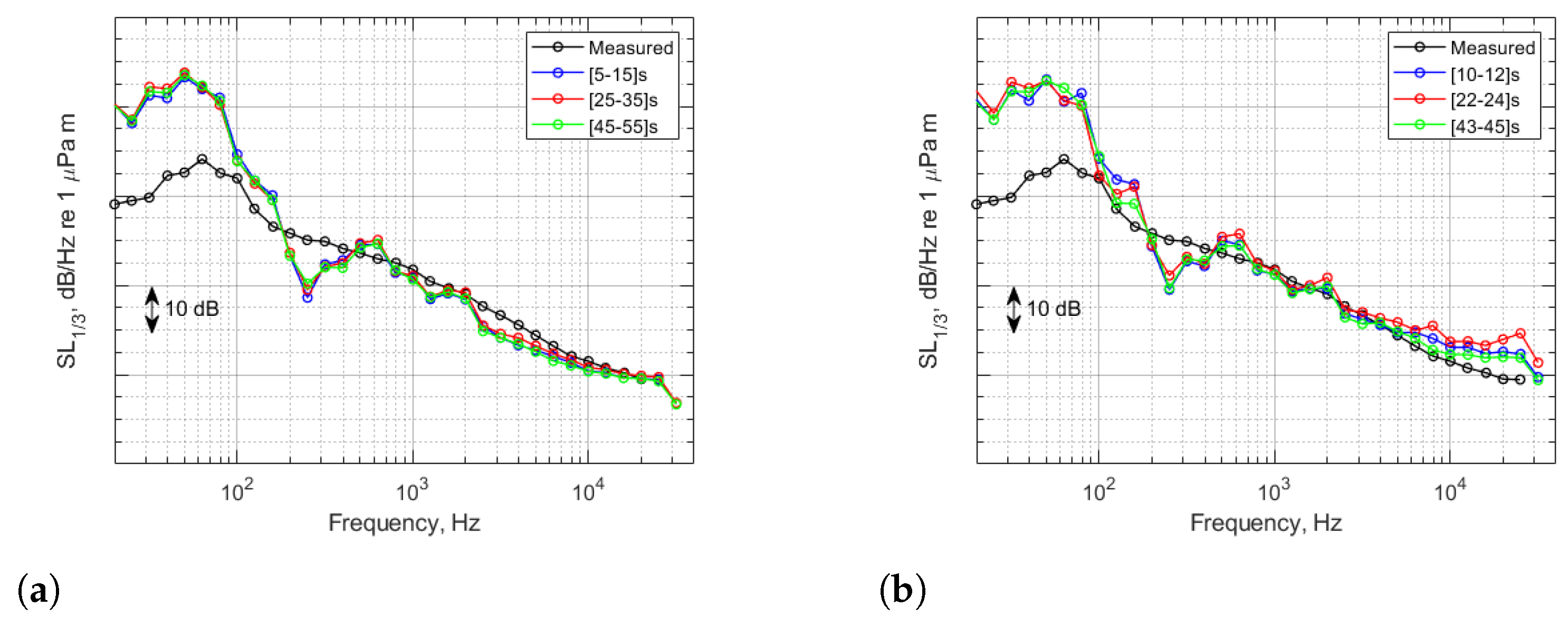
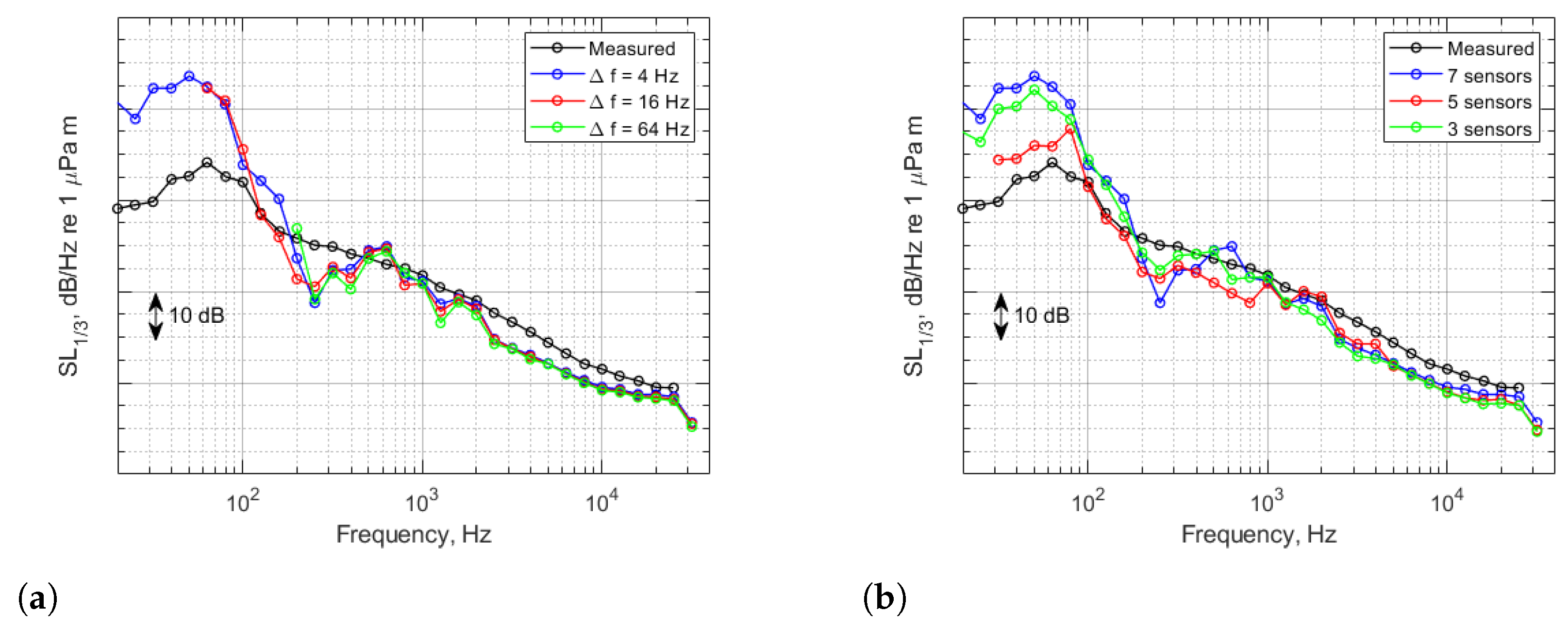
2.2. Validation of the Method
3. Source-Level Estimation at Full Scale
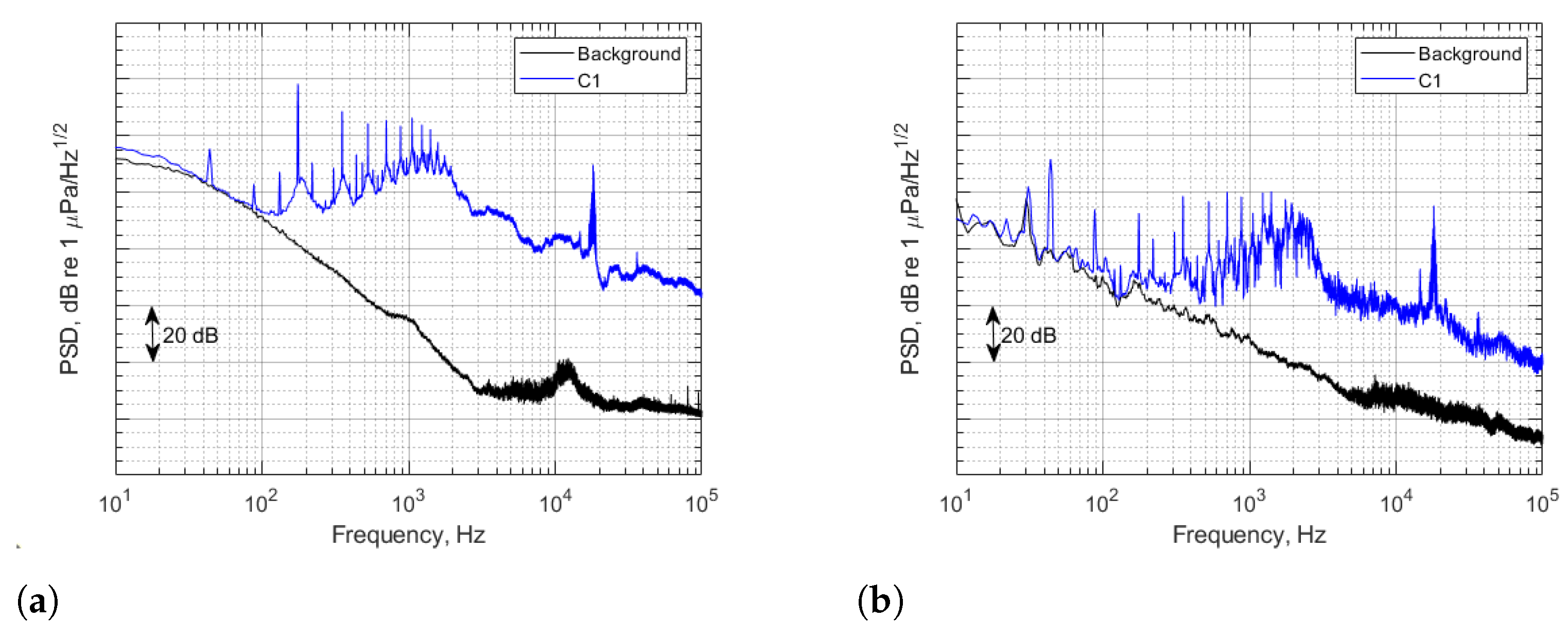
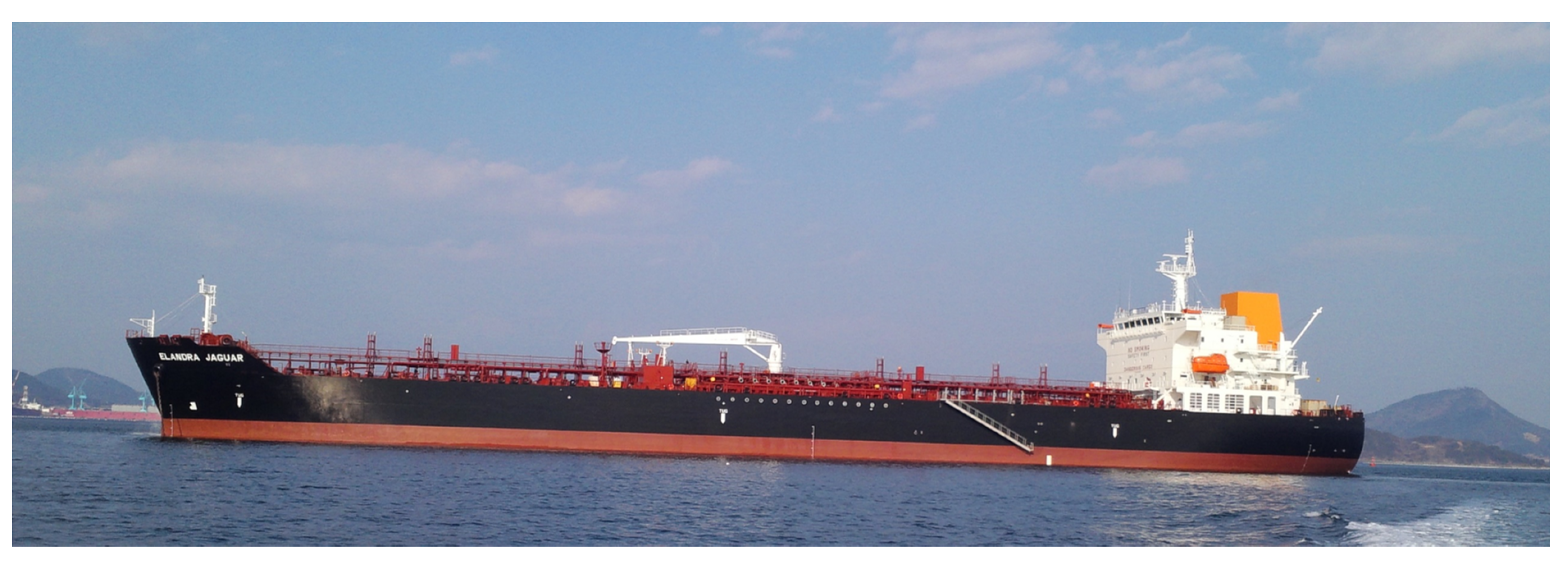
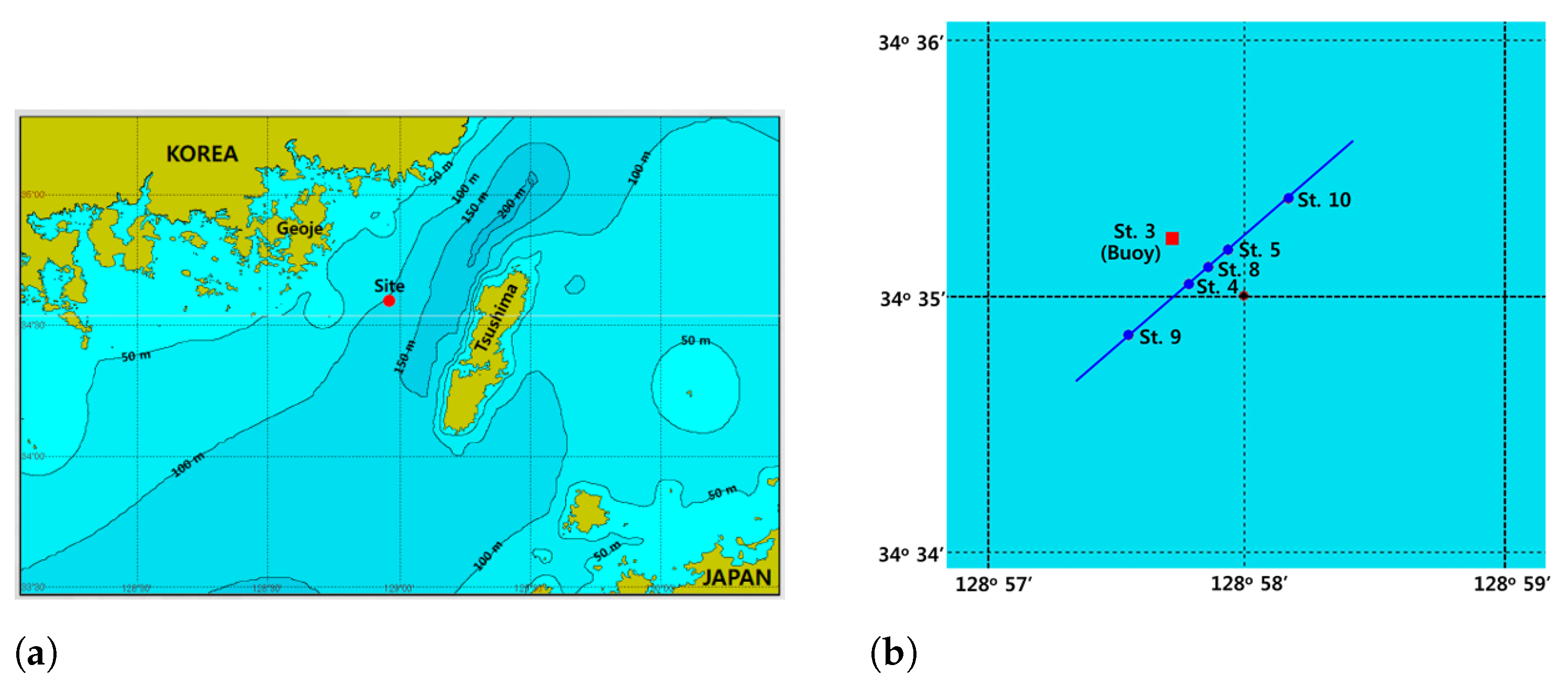
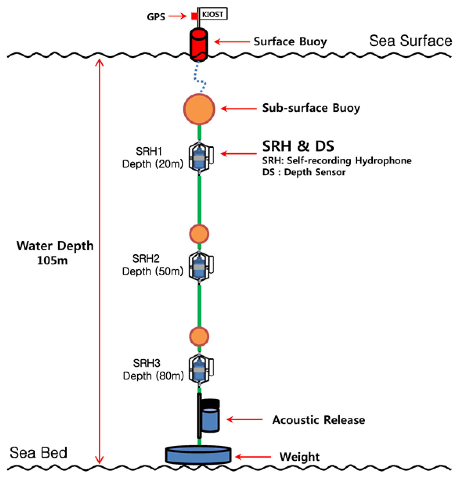
3.1. Underwater Radiated Noise (URN) Measurement
- For 3 dB: data to be discarded;
- For 10 dB 3 dB: = (dB);
- For 10 dB: no corrections.
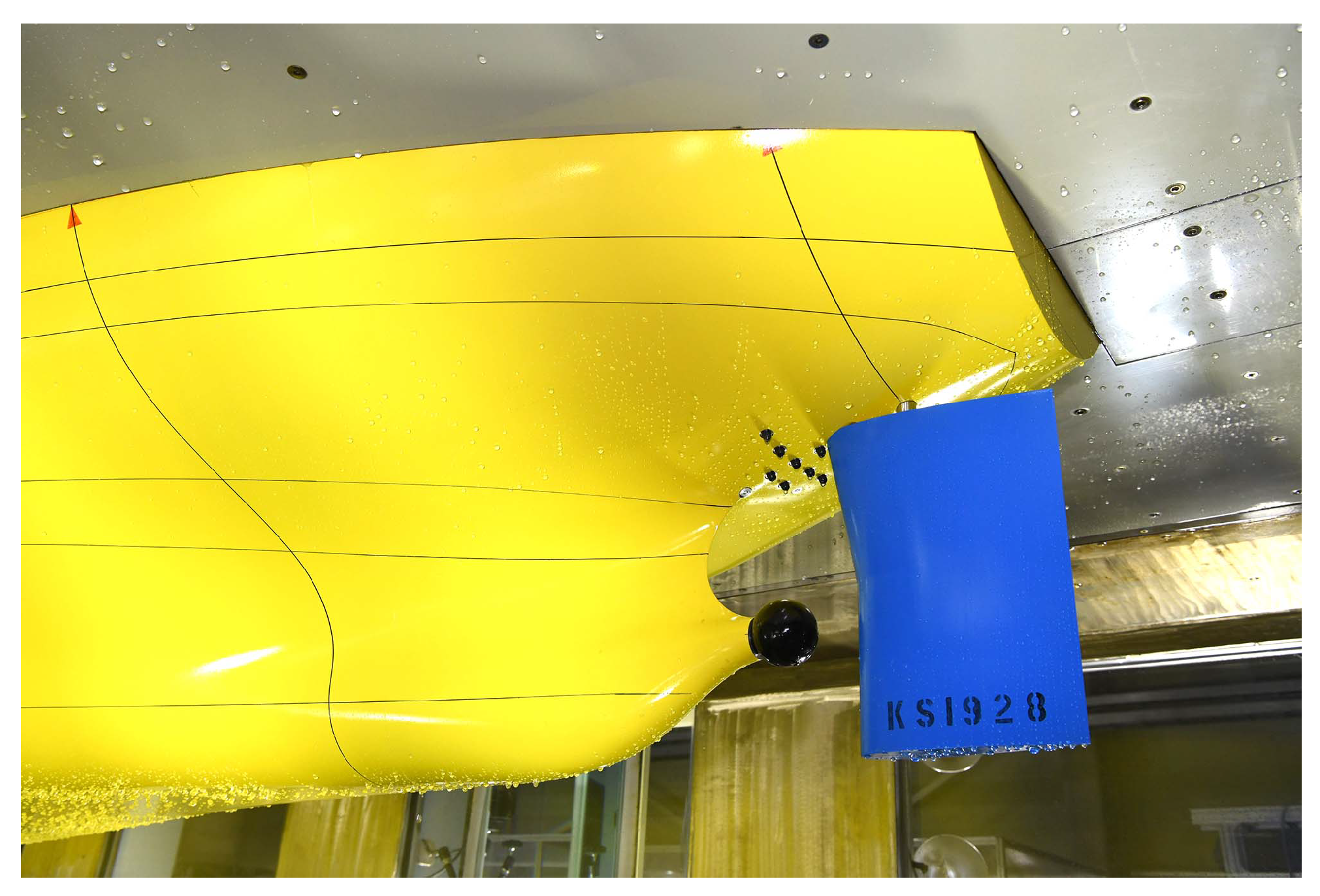
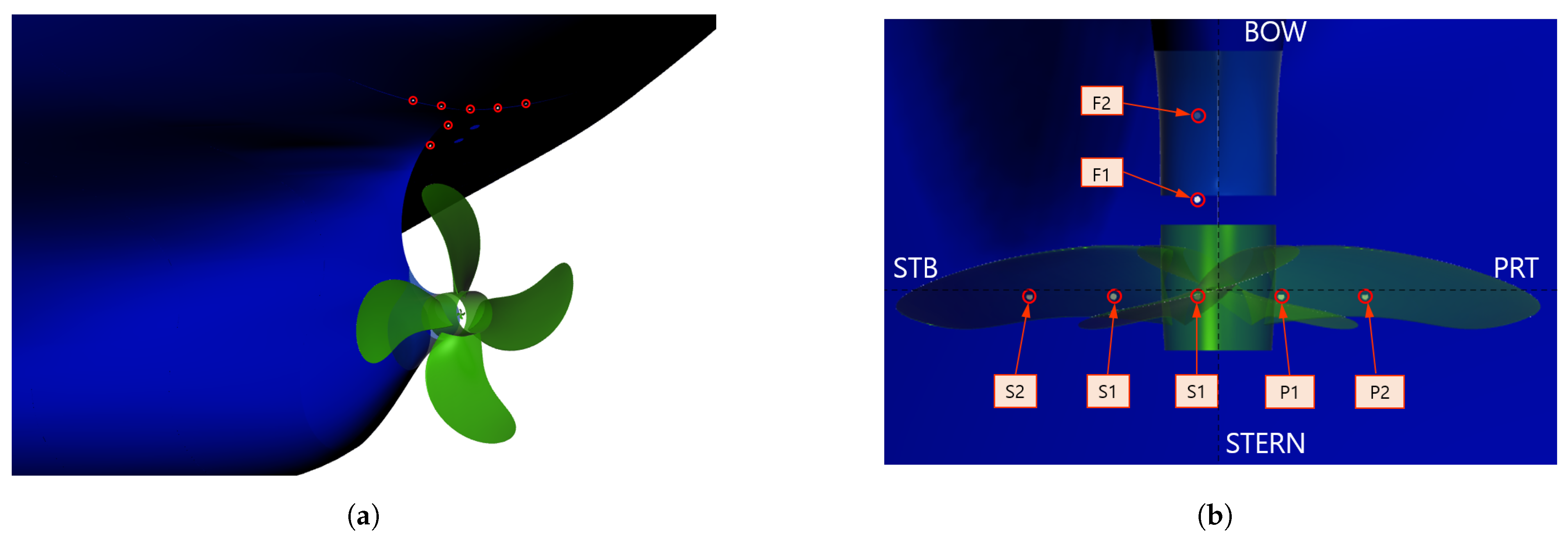
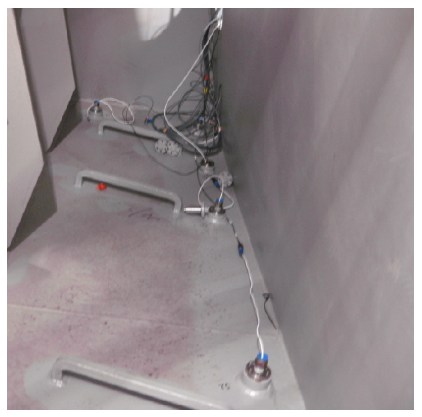
3.2. Hull Pressure Measurement
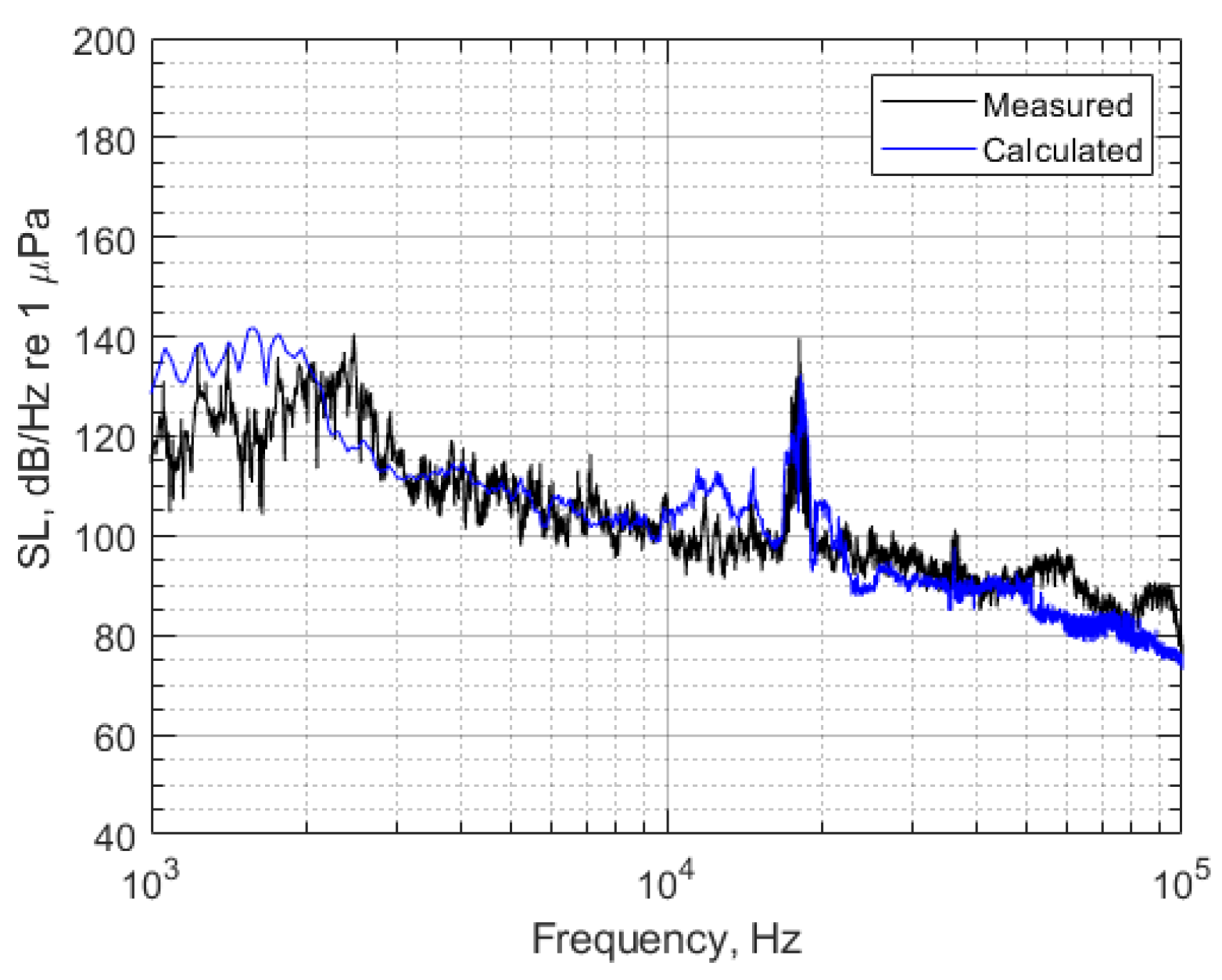
3.3. Results and Discussion
4. Conclusions
Author Contributions
Funding
Institutional Review Board Statement
Informed Consent Statement
Data Availability Statement
Acknowledgments
Conflicts of Interest
Abbreviations
| BPF | Blade-Passing Frequency |
| IMO | International Maritime Organization |
| ITTC | International Towing Tank Conference |
| KIOST | Korea Institute of Ocean Science and Technology |
| KRISO | Korea Research Institute of Ships and Ocean Engineering |
| LCT | Large Cavitation Tunnel |
| MVDR | Minimum-Variation Distortionless Response |
| PSD | Power Spectral Density |
| SL | Source Level |
| SPL | Sound Pressure Level |
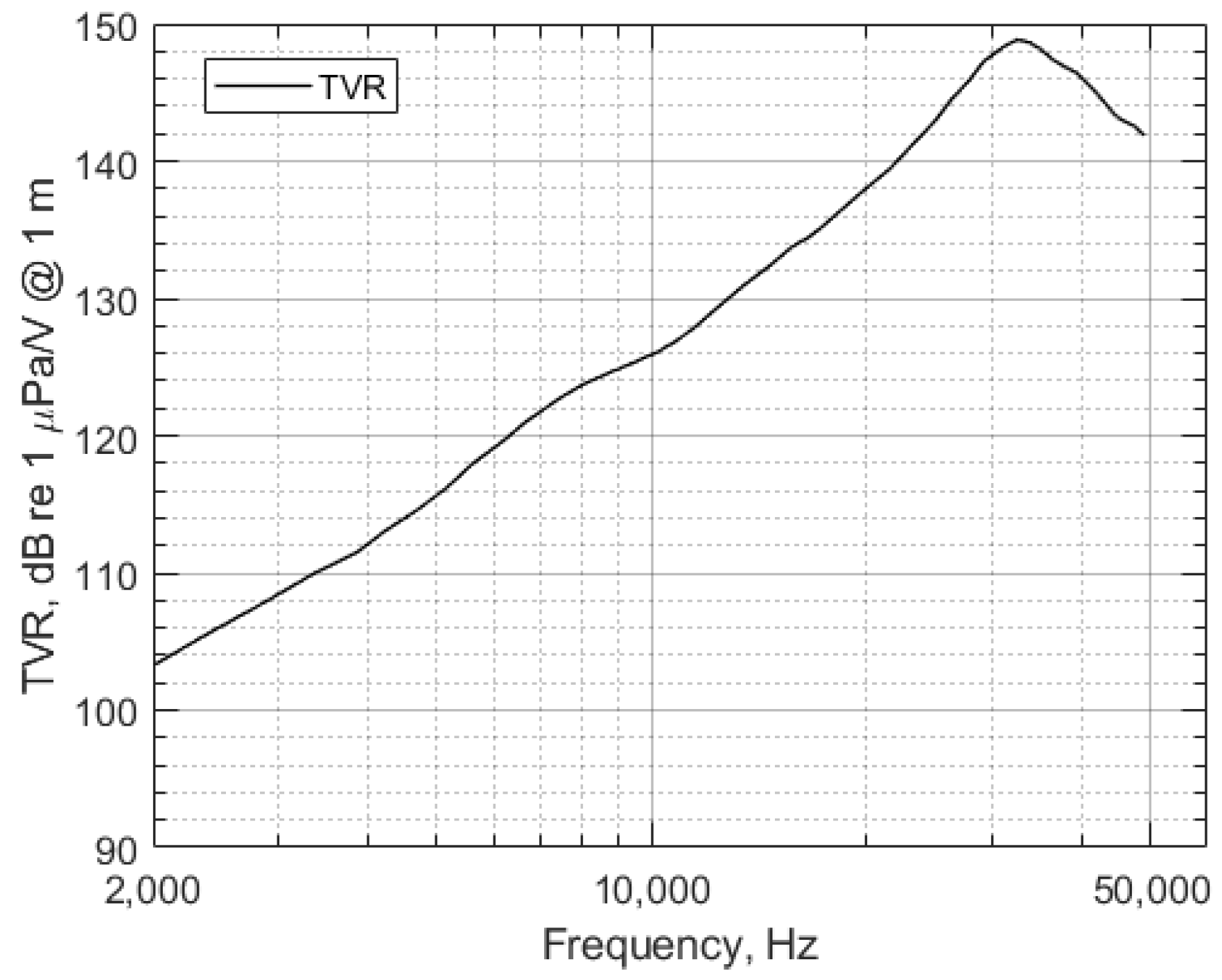
| TVR | Transmitting Voltage Response |
| URN | Underwater Radiated Noise |
References
- Kaplan, M.B.; Solomon, S. A coming boom in commercial shipping? The potential for rapid growth of noise from commercial ships by 2030. Mar. Policy 2016, 73, 119–121. [Google Scholar] [CrossRef]
- McDonald, M.A.; Hildebr, J.A.; Wiggins, S.M. Increases in deep ocean ambient noise in the Northeast Pacific west of San Nicolas Island, California. J. Acoust. Soc. Am. 2006, 120, 711–718. [Google Scholar] [CrossRef]
- Roll, R.M.; Parks, S.E.; Hunt, K.E.; Castellote, M.; Corkeron, P.J.; Nowacek, D.P.; Wasser, S.K.; Kraus, S.D. Evidence that ship noise increases stress in right whales. Proc. R. Soc. Biol. Sci. 2012, 279, 2363–2368. [Google Scholar]
- Cominelli, S.; Devillers, R.; Yurk, H.; MacGillivray, A.; McWhinnie, L.; Canessa, R. Noise exposure from commercial shipping for the southern resident killer whale population. Mar. Pollut. Bull. 2018, 136, 177–200. [Google Scholar] [CrossRef]
- ISO 17208-1:2016. Underwater Acoustics–Quantities and Procedures for Description and Measurement of Underwater Sound from Ships–Part 1: Requirements for Precision Measurements in Deep Water Used for Comparison Purposes; International Standard Organization: Geneva, Switzerland, 2016. [Google Scholar]
- Brooker, A.; Humphrey, V. Measurement of radiated underwater noise from a small research vessel in shallow water. Ocean Eng. 2016, 120, 182–189. [Google Scholar] [CrossRef]
- Humphrey, V.; Brooker, A.; Dambra, R.; Firenze, E. Variability of underwater radiated noise measured using two hydrophone arrays. In Proceedings of the OCEANS 2015-Genova, Genoa, Italy, 18–21 May 2015; pp. 1–10. [Google Scholar]
- Gassmann, M.; Wiggins, S.M.; Hildebr, J.A. Deep-water measurements of container ship radiated noise signatures and directionality. J. Acoust. Soc. Am. 2017, 142, 1563–1574. [Google Scholar] [CrossRef]
- Johansson, A.T.; Haller, J.; Karlsson, R.; Långström, A.; Turesson, M. Full scale measurement of underwater radiated noise from a coastal tanker. In Proceedings of the OCEANS 2015-Genova, Genoa, Italy, 18–21 May 2015; pp. 1–10. [Google Scholar]
- McKenna, M.F.; Ross, D.; Wiggins, S.M.; Hildebr, J.A. Underwater radiated noise from modern commercial ships. J. Acoust. Soc. Am. 2012, 131, 92–103. [Google Scholar] [CrossRef]
- Merchant, N.D.; Pirotta, E.; Barton, T.R.; Thompson, P.M. Monitoring ship noise to assess the impact of coastal developments on marine mammals. Mar. Pollut. Bull. 2014, 78, 85–95. [Google Scholar] [CrossRef]
- Garrett, J.K.; Blondel, P.; Godley, B.J.; Pikesley, S.K.; Witt, M.J.; Johanning, L. Long-term underwater sound measurements in the shipping noise indicator bands 63 Hz and 125 Hz from the port of Falmouth Bay, UK. Mar. Pollut. Bull. 2016, 110, 438–448. [Google Scholar]
- The Specialist Committee on Hydrodynamic Noise: Final Report and Recommendations to the 28th ITTC. 2017. Available online: www.ittc.info/media/7837/17-sc-hydrodynamic-noise-compressed.pdf (accessed on 26 January 2021).
- Seol, H.; Paik, B.-G.; Park, Y.-H.; Kim, K.-Y.; Ahn, J.-W.; Park, C.-S.; Kim, G.-D.; Kim, K.-S. Propeller cavitation noise model test in KRISO large cavitation tunnel and its comparison with full-scale results. In Proceedings of the 4th International Conference on Advanced Model Measurement Technology for the Maritime Industry, Istanbul, Turkey, 28–30 September 2015. [Google Scholar]
- Haller, J.; Johansson, A.T. Underwater Radiated Noise Measurements on a Chemical Tanker—Comparison Full-Scale and Model-Scale Results. In Proceedings of the 4th International Conference on Advanced Model Measurement Technology for the Maritime Industry, Istanbul, Turkey, 28–30 September 2015. [Google Scholar]
- Aktas, B.; Atlar, M.; Turkmen, S.; Shi, W.; Sampson, R.; Korkut, E.; Fitzsimmons, P. Propeller cavitation noise investigations of a research vessel using medium size cavitation tunnel tests and full-scale trials. Ocean Eng. 2016, 120, 122–135. [Google Scholar] [CrossRef]
- Lafeber, F.H.; Bosschers, J. Validation of computational and experimental prediction methods for the underwater radiated noise of a small research vessel. In Proceedings of the 13th International Symposium on PRActical Design of Ships and Other Floating Structures (PRADS’ 2016), Copenhagen, Denmark, 4–8 September 2016. [Google Scholar]
- Tani, G.; Viviani, M.; Felli, M.; Lafeber, F.H.; Lloyd, T.; Aktas, B.; Atlar, M.; Turkmen, S.; Seol, H.; Hallander, J.; et al. Noise measurements of a cavitating propeller in different facilities: Results of the round robin test programme. Ocean Eng. 2020, 213, 107599. [Google Scholar] [CrossRef]
- Bosschers, J. A semi-empirical prediction method for broadband hull-pressure fluctuations and underwater radiated noise by propeller tip vortex cavitation. J. Mar. Sci. Eng. 2018, 6, 49. [Google Scholar] [CrossRef]
- Seol, H.; Suh, J.C.; Lee, S. Development of hybrid method for the prediction of underwater propeller noise. J. Sound Vib. 2005, 288, 345–360. [Google Scholar] [CrossRef]
- Kellet, P.; Turan, O.; Incecik, A. A study of numerical ship underwater noise prediction. Ocean Eng. 2013, 66, 113–120. [Google Scholar] [CrossRef]
- Wu, Q.; Huang, B.; Wang, G.; Cao, S.; Zhu, M. Numerical modelling of unsteady cavitation and induced noise around a marine propeller. Ocean Eng. 2018, 160, 143–155. [Google Scholar]
- Li, D.Q.; Haller, J.; Johhanson, T. Predicting underwater radiated noise of a full scale ship with model testing and numerical methods. Ocean Eng. 2018, 161, 121–135. [Google Scholar] [CrossRef]
- Ten Wolde, T.; De Bruijn, A. A new method for the measurement of the acoustical source strength of cavitating ship propellers. Int. Shipbuild. Prog. 1975, 22.255, 385–396. [Google Scholar] [CrossRef]
- Van Wijngaarden, E. Determination of Propeller Source Strength from Hull-Pressure Measurements. In Proceedings of the Lloyd’s List Conference on Noise and Vibration in the Marine Environment, London, UK, 28–29 June 2006. [Google Scholar]
- Lee, K.; Lee, J.; Kim, D.; Kim, K.; Seong, W. Propeller sheet cavitation noise source modeling and inversion. J. Sound Vib. 2014, 333, 1356–1368. [Google Scholar] [CrossRef]
- Ahn, B.K.; Go, Y.G.; Rhee, W.; Choi, J.S.; Lee, C.S. Localization of underwater noise sources using TDOA (Time Difference of Arrival) method. J. Soc. Nav. Archit. Korea 2011, 48, 121–127. [Google Scholar] [CrossRef][Green Version]
- Choo, Y.; Seong, W. Compressive spherical beamforming for localization of incipient tip vortex cavitation. J. Acoust. Soc. Am. 2016, 140, 4085–4090. [Google Scholar] [CrossRef]
- Lee, J.H.W. Acoustic localization of incipient cavitation in marine propeller using greedy-type compressive sensing. Ocean. Eng. 2020, 197, 106894. [Google Scholar] [CrossRef]
- Turkmen, S.; Aktas, B.; Atlar, M.; Sasaki, N.; Sampson, R.; Shi, W. On-board measurement techniques to quantify underwater radiated noise level. Ocean Eng. 2017, 130, 166–175. [Google Scholar] [CrossRef]
- Foeth, E.J.; Bosschers, J. Localization and Source-Strength Estimation of Propeller Cavitation Noise Using Hull-Mounted Pressure Transducers. In Proceedings of the 31st Symposium on Naval Hydrodynamics, Monterey, CA, USA, 11–16 September 2016; pp. 11–16. [Google Scholar]
- Ahn, J.-W.; Paik, B.-G.; Seol, H.; Kim, G.-D.; Kim, K.-S.; Jung, B.-J.; Choi, S.-J. Comparative study of full-scale propeller cavitation test and LCT model test for MR Tanker. J. Soc. Nav. Archit. Korea 2016, 53, 180–188. [Google Scholar]


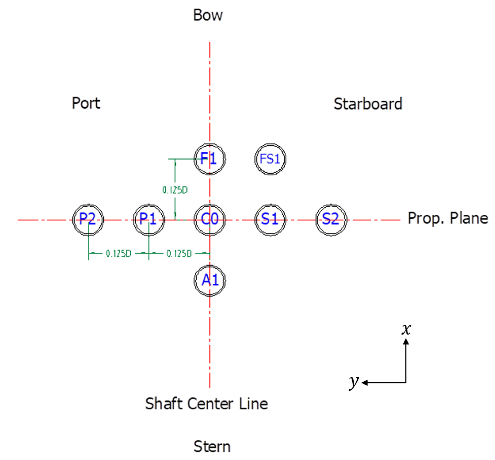
| Position | x (mm) | y (mm) |
|---|---|---|
| P2 | 0 | 62.5 |
| P1 | 0 | 31.25 |
| C0 | 0 | 0 |
| S1 | 0 | −31.25 |
| S2 | 0 | −62.5 |
| F1 | 31.25 | 0 |
| A1 | −31.25 | 0 |
| FS1 | 31.25 | −31.25 |
| Condition | V (m/s) | n (rps) | |
|---|---|---|---|
| 7.0 | 3.06 | 44.04 | |
| 7.0 | 2.82 | 44.16 | |
| 7.0 | 2.61 | 44.30 |
| Position | x (mm) | y (mm) |
|---|---|---|
| P2 | −78 | 1400 |
| P1 | −78 | 600 |
| C0 | −78 | −200 |
| S1 | −78 | −1000 |
| S2 | −78 | −1800 |
| F1 | 848 | −200 |
| F2 | 1648 | −200 |
| Octave Band | -, dB | ||
|---|---|---|---|
| Center Frequency, Hz | |||
| 31.5 | 24.8 | 24.4 | 25.1 |
| 63 | 16.6 | 15.8 | 17.9 |
| 125 | 7.1 | 6.0 | 7.4 |
| 250 | −12.6 | ||
| 500 | 1.8 | 1.6 | 2.0 |
| 1000 | 0.1 | ||
| 2000 | 1.4 | 4.3 | |
| 4000 | |||
| 8000 | |||
| 16,000 | |||
| Parameter | Range |
|---|---|
| Recording time (), s | 60, 10, 2 |
| Frequency resolution (), Hz | 4, 16, 64 |
| Number of sensors | 7, 5, 3 |
Publisher’s Note: MDPI stays neutral with regard to jurisdictional claims in published maps and institutional affiliations. |
© 2021 by the authors. Licensee MDPI, Basel, Switzerland. This article is an open access article distributed under the terms and conditions of the Creative Commons Attribution (CC BY) license (http://creativecommons.org/licenses/by/4.0/).
Share and Cite
Jeong, H.; Lee, J.-H.; Kim, Y.-H.; Seol, H. Estimation of the Noise Source Level of a Commercial Ship Using On-Board Pressure Sensors. Appl. Sci. 2021, 11, 1243. https://doi.org/10.3390/app11031243
Jeong H, Lee J-H, Kim Y-H, Seol H. Estimation of the Noise Source Level of a Commercial Ship Using On-Board Pressure Sensors. Applied Sciences. 2021; 11(3):1243. https://doi.org/10.3390/app11031243
Chicago/Turabian StyleJeong, Hongseok, Jeung-Hoon Lee, Yong-Hyun Kim, and Hanshin Seol. 2021. "Estimation of the Noise Source Level of a Commercial Ship Using On-Board Pressure Sensors" Applied Sciences 11, no. 3: 1243. https://doi.org/10.3390/app11031243
APA StyleJeong, H., Lee, J.-H., Kim, Y.-H., & Seol, H. (2021). Estimation of the Noise Source Level of a Commercial Ship Using On-Board Pressure Sensors. Applied Sciences, 11(3), 1243. https://doi.org/10.3390/app11031243