Numerical Study on the Route of Flame-Induced Thermoacoustic Instability in a Rijke Burner

Abstract

The self-excited thermoacoustic instability in a two-dimensional Rijke-type burner with a center-stabilized premixed methane–air flame is numerically studied. The simulation considers the reacting flow, flame dynamics, and radiation model to investigate the important physical processes. A finite volume-based approach is used to simulate reacting flows under both laminar and turbulent flow conditions. Chemical reaction modeling is conducted via the finite-rate/eddy dissipation model with one-step reaction mechanisms, and the radiation heat flux and turbulent flow characteristics are determined by using the P-1 model and the standard k-ε model, respectively. The steady-state reacting flow is first simulated for model verification. Then, the dynamic pressure, velocity, and reaction heat evolutions are determined to show the onset and growth rate of self-excited instability in the burner. Using the fast Fourier transform (FFT) method, the frequency of the limit cycle oscillation is obtained, which agrees well with the theoretical prediction. The dynamic pressure and velocity along the tube axis provide the acoustic oscillation mode and amplitude, also agreeing well with the prediction. Finally, the unsteady flow field at different times in a limit cycle shows that flame-induced vortices occur inside the combustor, and the temperature distribution indicates that the back-and-forth velocity changes in the tube vary the distance between the flame and honeycomb in turn, forming a forward feedback loop in the tube. The results reveal the route of flame-induced thermoacoustic instability in the Rijke-type burner and indicate periodical vortex formation and breakdown in the Rijke burner, which should be considered turbulent flow under thermoacoustic instability.

1. Introduction

In 1859, Rijke discovered strong acoustic oscillations when heat was added to the lower half of a vertical tube opened at both ends [1]. Several similar devices were proposed to study the heat-driven acoustic phenomenon in past decades, and these devices were grouped under the general heading “Rijke tube” [2]. Among these devices, one type in which the flow is combustible gas and the heat is produced by the flame is called a Rijke burner or a Rijke tube burner.

Experimental research on the Rijke burner is intuitive and can yield highly reliable information about thermoacoustic instability, such as temperature, pressure, and velocity. Abundant nonlinear behaviors, such as limit cycle oscillation, quasiperiodic, frequency-locked, and chaotic behaviors, were discovered [3,4,5]. Based on experimental results, some classical flame models have been proposed [6,7,8,9,10]. However, experimental methods can collect data only at finite points. The parameters of the entire field cannot be obtained by experimental methods, and a comprehensive understanding of the flow field of thermoacoustic instability is still lacking.

Analytical studies have been conducted to explain the mechanisms of thermoacoustic instability since the 1960s [11,12]. Culick established the linear theory of combustion instabilities and first derived the nonlinear acoustic model in combustion chambers based on experimental research [13,14,15,16]. Balasubramanian and Sujith investigated the role of nonnormality and nonlinearity in flame–acoustic interactions and found that nonnormality and nonlinearity lead to triggering and redistribution of energy between eigenmodes [17]. Yoon et al. predicted the bootstrapping instability mechanism observed in rocket motors by approximated modal analysis [18,19]. Li et al. observed the stability switch phenomenon with a one-dimensional (1-D) Rijke-type thermoacoustic system [20]. Through the analytical method, we have obtained a thoughtful understanding of the mechanism of thermoacoustic instability, especially for predicting the frequency, amplitude, and stability of self-excited thermoacoustic instability.

With the development of computational technology, computational fluid dynamics (CFD) simulations have increasingly helped to describe the mechanisms of thermoacoustic instability and to provide guidance for experimental research, making up for the shortage of experimental work.

Many numerical studies have been conducted on combustion instabilities. Because of the nonlinearity in the combustion system, the interactions between reaction mechanisms, hydrodynamics, and acoustics reveal different spatial and temporal scales and are sensitive to various parameters. Chatterjee investigated the occurrence of combustion instabilities in a Rijke tube-type combustor using a two-dimensional (2-D) finite volume method, captured the instability growth to a limit cycle of the pressure oscillation, and predicted the frequency and magnitude of the thermoacoustic instability [21]. Chatterjee et al. simulated a three-dimensional (3-D) premixed chamber with ANSYS FLUENT software and studied the dependence of a homogeneous mixture on various parameters such as the premixing length, airflow rate, and equivalence ratio to optimize the combustor [22]. Wang also successfully simulated the lean premixed combustion instabilities in a 2-D Rijke-type burner by CFD simulation and found that the radiation and reaction mechanism play critical roles in predicting the occurrence of thermoacoustic instability [23]. Blanchard et al. simulated a bluff-body flame holder, and the proper orthogonal decomposition modes of the simulated results and experiments showed quantitative agreement [24]. Ghulam et al. used COMSOL software to investigate the driving mechanism of combustion instabilities in a small rectangular combustion duct and obtained the pressure waves in the longitudinal and transverse directions [25]. On the research of the interaction of turbulence and combustion, numerical simulation has also shown its extraordinary ability [26]. These CFD simulations help in understanding the detailed flow parameters, such as pollution control, efficiency enhancement, and mass transport processes, for further analysis and can thus serve as an aid to engineers and designers for building combustion systems with a decreased possibility of thermoacoustic instabilities.

The present study concentrates on the numerical simulation of a 2-D Rijke burner to understand the dynamics of self-excited thermoacoustic instability. A finite volume- based approach is used to simulate reacting flows under both laminar and turbulent flow conditions. The onset of growth of the pressure, velocity, and reaction heat are captured. The oscillation frequency and mode are calculated and compared with the theoretical prediction, and they show good agreement. Finally, the unsteady flow fields at different times show that flame-induced vortices occur inside the combustor, and the temperature distributions show that the velocity perturbation in the tube changes the distance between the flame and honeycomb in turn, forming a forward feedback loop in the tube. The results of this work show that there are vortices in the Rijke-type burner when thermoacoustic instability occurs, and it should be considered a turbulent reacting flow field.

2. Numerical Model

2.1. Rijke Burner Configuration

The Rijke burner used in this study consists of a 1572 mm-long steel tube with an inner diameter of 73.7 mm, as shown in Figure 1. A premixed methane–air mixture is fed into the inlet end of the tube, and a honeycomb flame stabilizer with a thickness of 25.4 mm is positioned in the middle of the tube. A flat flame is anchored at the top of the honeycomb flame stabilizer, and releases unsteady heat into the flow, inducing pressure oscillation in the tube. A 2-D axisymmetric flow field is used to approximate the 3-D flow field to simplify the computational model as shown in Figure 2.

The model of the Rijke burner is generated, and boundary conditions are set, including the mass flow rate inlet, pressure outlet, coupled wall between the honeycomb and flow, coupled wall between the inside tube wall and flow, outer tube walls, and axisymmetric centerline. The input parameters used in setting up the Rijke burner mode are as follows. The incoming flow is set to 1.27 × 10⁻⁴ kg/s with a fuel/air equivalence ratio of 0.75. The equivalence ratio is defined as the value of the actual fuel/air mass ratio relative to stoichiometric fuel/air ratio. If it is less than 1, the combustion is lean with excess air. The convective heat transfer coefficient for the outside tube wall is estimated to be 20 W/(m²·K), and the reference condition is set as normal temperature and pressure. The boundary conditions and initial conditions are summarized in

Table A1. Operational conditions for the Rijke burner simulation.

Boundary	Boundary Condition	Parameter Setting
Inlet	Uniform and steady velocity Acoustically closed	1.27 × 10−4 kg/s $u^{\prime }=0\mathrm{m}/\mathrm{s}$
	Fuel–air mass fractions	CH4: 0.04197 O2: 0.22323 $(\mathsf{\Phi }=0.75)$
	Temperature of the mixture	293 K
Outlet	Atmospheric pressure Acoustically open	0 Pa (gauge pressure)
	Species mass fractions	O2: 0.23292
Inside tube wall	Coupled between the fluid flow and the adjoining solid wall
Outside tube wall	Convection coefficient	20 W/(m2∙K)
Flame stabilizer wall	Coupled between the fluid flow and the adjoining solid wall
Centerline	Axisymmetric boundary

and

Table A2. Operational conditions for the Rijke burner simulation.

Simulation Stage	Initial Condition
Stage 1: Steady-state reacting flow simulation	The inlet parameter
Stage 2: Unsteady reacting flow simulation	The result of the steady state solution

of Appendix A, respectively.

2.2. Mathematical Model

The governing equations of this model include conservation equations of mass, kinetics, species, and energy, combined with turbulence equations and radiation equations. The conservation equations are expressed by

$$\frac{\partial \left(\rho \Phi \right)}{\partial t}+div\left(\rho u\Phi \right)=div\left(\Gamma grad\Phi \right)+S_{\Phi }$$

(1)

where $\rho$, $t$, and $u$ are the density, time, and velocity, respectively; $\Phi$ represents the dependent transport variables [27]; $\Gamma$ represents the diffusion coefficient; and $S_{\Phi }$ is the source term of the variable $\Phi$.

The governing equations are solved with the finite volume method. Although at the steady state of the combustion field the average velocity is approximately 0.026 m/s, the corresponding Reynolds number is approximately 120, and the Mach number is 1.5 × 10⁻⁴ in this model, indicating that this is a laminar flow for the non-reacting condition. However, influenced by the highly nonlinear chemical reaction, it is inappropriate to ignore the turbulence effect in this model. The k-ε model [28] is the most common model used in CFD to simulate mean flow characteristics for turbulent flow conditions. Here, the k-ε model with enhanced wall treatment is used to simulate the reacting flow.

The species is determined by the species transport model, while the finite-rate/eddy dissipation model is applied to compute the interaction between turbulence and chemistry. Besides, the material properties used are listed in

Table A3. Material properties for the Rijke burner simulation.

Material	Properties	Unit	Parameter Setting
Fuel-air mixture	Density	kg/m3	Ideal gas
	Specific heat (Cp)	J/(kg∙K)	Mixing law
	Thermal conductivity	W/(m∙K)	Ideal gas mixing law
	Viscosity	kg/(ms)	Ideal gas mixing law
	Mass diffusivity	m2/s	Kinetic-theory
	Thermal diffusion coeff.	kg/(ms)	Kinetic-theory
	Reaction		One-step finite-rate reaction
	Radiation		P-1
Tube wall	Material		Carbon steel
	Height	mm	1572
	Inner diameter	mm	73.7
	Wall thickness	mm	7.62
	Density	kg/m3	8030.0
	Thermal conductivity	W/(m∙K)	16.27
	Specific heat (Cp)	J/(kg∙K)	502.48
Flame stabilizer	Material		Cordierite
	Thickness	mm	25.4
	Diameter	mm	73.7
	Density	kg/m3	2300
	Thermal conductivity	W/(m∙K)	2.28228
	Specific heat (Cp)	J/(kg∙K)	850.63
	Area restriction		50%

of Appendix A.

The methane/air reaction is complicated and involves dozens of reactions and hundreds of elementary reactions. Several reaction mechanisms have been proposed to accurately describe the combustion process. The detailed reaction mechanisms are highly precise [29], while the computational costs are increased. In a numerical comparison between the different methane/air combustion mechanisms, Li [30] pointed out that the one-step mechanism agrees with experimental results quantitatively for fuel-lean conditions. Acampora et al. [31] concluded that moving from a one-step global mechanism to a two-step mechanism does not significantly increase the accuracy of predictions. According to the mentioned points, the one-step reaction mechanism is used for the reaction of methane and air, and is expressed as

$$C{H}_4+2\left(O_2+3.76N_2\right)\stackrel{K_G}{\to }C{O}_2+2H_{2}O+7.52N_2$$

(2)

The rate of fuel consumption is given by the global Arrhenius equation:

$$\frac{\mathrm{d}\left[C{H}_4\right]}{\mathrm{d}t}=-Aexp\left(\frac{-E_a}{R_{u}T}\right){\left[C{H}_4\right]}^m{\left[O_2\right]}^n$$

(3)

where the parameters A, $E_a/R_u$, m and n are given in

Table A4. Parameters of the chemistry model for the methane and air reaction.

Pre-Exponential Factor. $\mathbf{A}\left[{\left(\mathbf{k}\mathbf{m}\mathbf{o}\mathbf{l}/{\mathbf{m}}^3\right)}^{\left(1-\mathbf{m}-\mathbf{n}\right)}/\mathbf{s}\right]$	Activation Temperature Ea/Ru [K]	m	n
2.119 × 1011	24,379	0.2	0.3

of Appendix A [32,33].

Due to the high temperatures of the flame, radiative heat transfer becomes one of the dominant mechanisms of heat transfer in addition to conduction and convection heat transfer [34,35]. Hence, proper simulation of the radiative heat transfer is of great importance to this problem. The P-1 model is based on the expansion of the radiation intensity I into an orthogonal series of spherical harmonics and has high accuracy and the ability to consider the radiation exchange in the flame environment [36,37,38,39] For this advantage, the P-1 model is widely used in the simulation of combustion [40,41]. In this work, the P-1 radiation model was chosen to model the high-temperature flow problem.

3. Results and Analysis

3.1. Grid Independence and Model Verification

To verify the computational model and grid independence, the numerical results of the axial temperature distribution at the centerline under steady-state combustion are compared. Three different numbers of nodes, namely, 26,312, 67,056, and 195,233 nodes, are compared with the previous numerical modeling of Wang [23], and the results are presented in Figure 3. The convergence limit is assumed when the residual values are less than 10⁻⁶.

As shown in Figure 3, the temperature distributions before the flame stabilizer almost converged to the same value, while in the flame stabilizer area and the flame zone, the temperature increased sharply because of the heat released by the flame. The result of the 67,056-node scheme is closer to the result presented by Wang [23] than the other two grid schemes.

The peak temperatures of the computational grids with 26,312, 67,056, and 195,233 nodes were approximately 1804 K, 1847 K, and 1908 K, respectively, and the outlet temperatures were 408 K, 331 K, and 354 K, while the peak temperature and outlet temperature in Wang’s simulation were 1927 K and 320 K, respectively. In addition, for the outlet temperature, the result of the 67,056-node scheme is much closer to the result of Wang. Consequently, the mesh with 67,056 nodes was selected as the best computation grid for computational modeling.

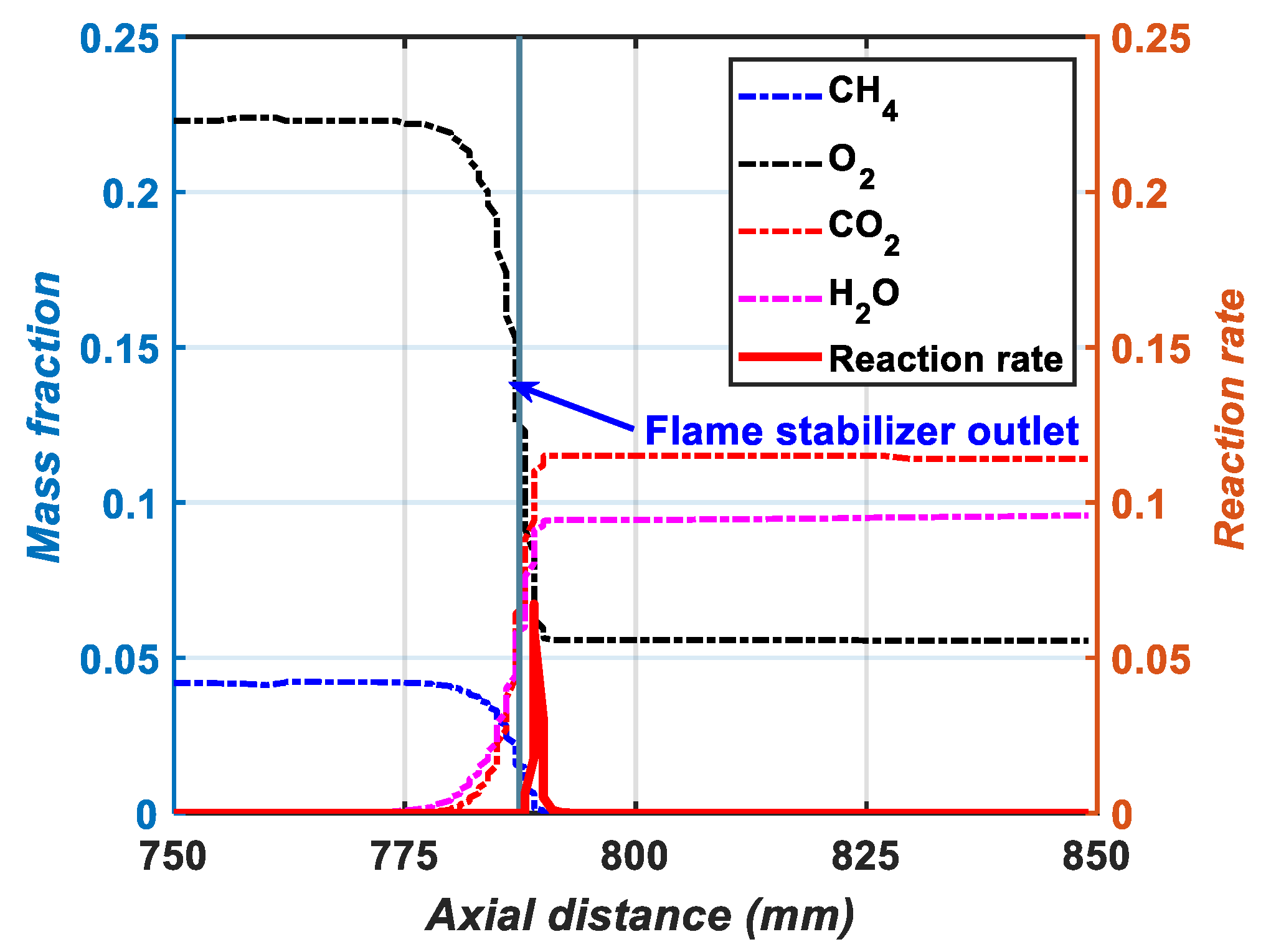
3.2. Steady-State Solution

The modeling of thermoacoustic instability proceeded in two stages—the first stage was the simulation of the steady-state reacting flow, and the second stage was the simulation of the transient reacting flow. For the steady-steady reaction simulation, the flow field was initialized with the inlet parameters. The solution of the steady-state reacting flow included the accurate capture of the flame anchoring process shown in Figure 4 and Figure 5, the consumption of reactants and product formation shown in Figure 6, and the steady-state temperature distribution along the combustor shown in Figure 3. Each process/distribution is important for verification of the computational results against the theoretical and experimental results.

The reaction rate and temperature contour plots downstream of the flame stabilizer are shown in Figure 4 and Figure 5, in which the location of the highest reaction rate and the temperature indicate the flame location. As seen in the figures, the flame sits just on the outlet of the flame stabilizer at a distance of 1–2 mm away from it. The temperature contours show that the incoming flow was preheated to approximately 800 K at the outlet of the honeycomb and then heated to a peak temperature of 1828 K by the reaction. Then, a steep temperature gradient, which was dominated by radiation heat transfer, occurred downstream of the peak temperature point. With decreasing temperature, the influence of radiation weakens, and the temperature gradient becomes increasingly gentle until the flow reaches the outlet.

The mass fractions of reactants and products along the centerline in the flame stabilizer area and the flame zone are shown in Figure 6. Due to the preheating effect of the flame stabilizer and flame radiation, the reaction started before the flame stabilizer outlet and rapidly increased to a peak downstream of it. At the flame location, the reaction rate reached its maximum value; the CH₄ fuel was completely consumed, and its mass fraction became zero. The steady-state species distribution and kinetic reaction rate show the exact location of the flame and demonstrate the effectiveness of the numerical simulation in this work.

In addition, the average flow velocity in the tube of the cold flow and steady-state reacting flow was obtained. The results show that the average velocity increased from 0.0257 to 0.071 m/s because the heat released from the flame heated and expanded the flow.

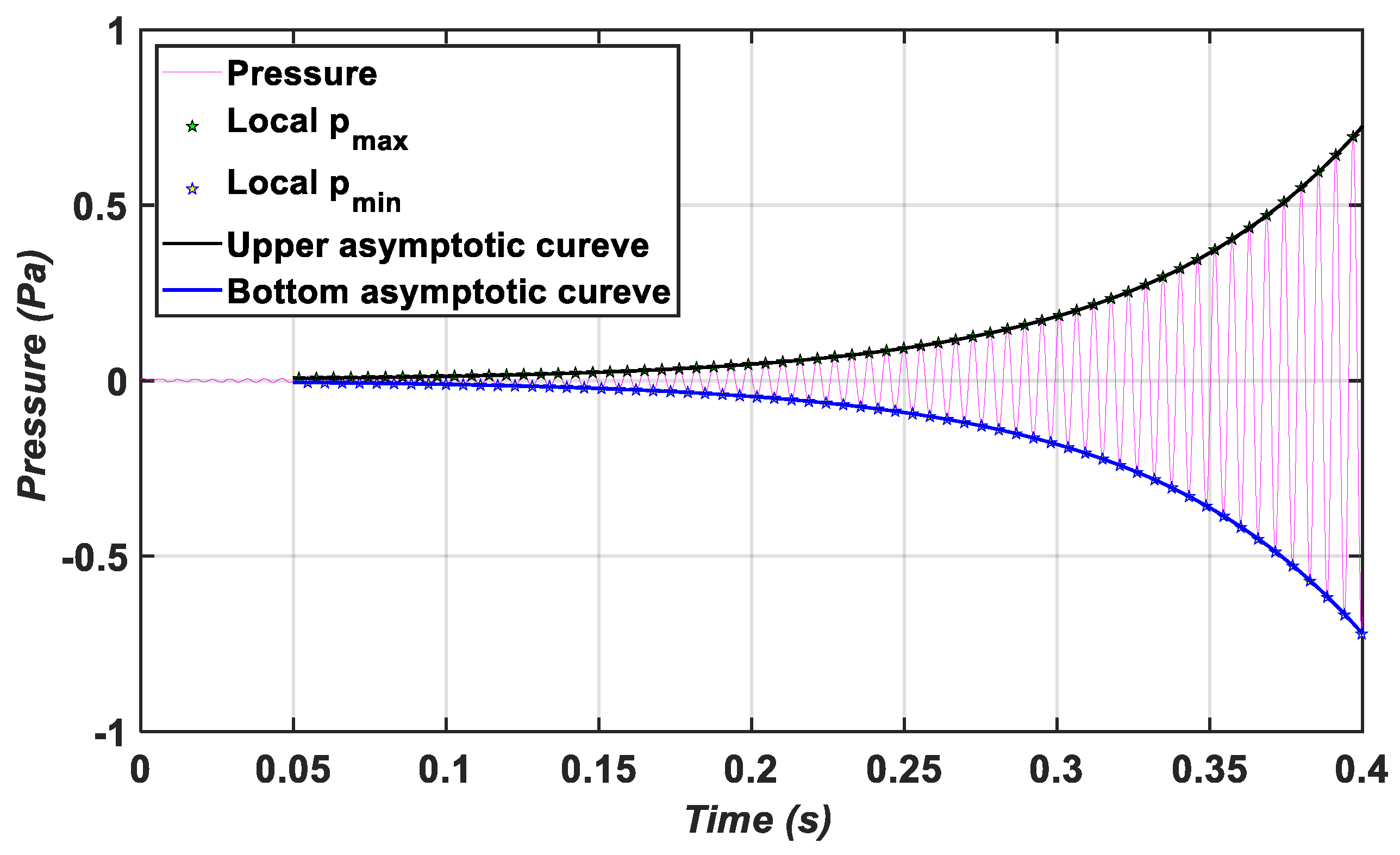
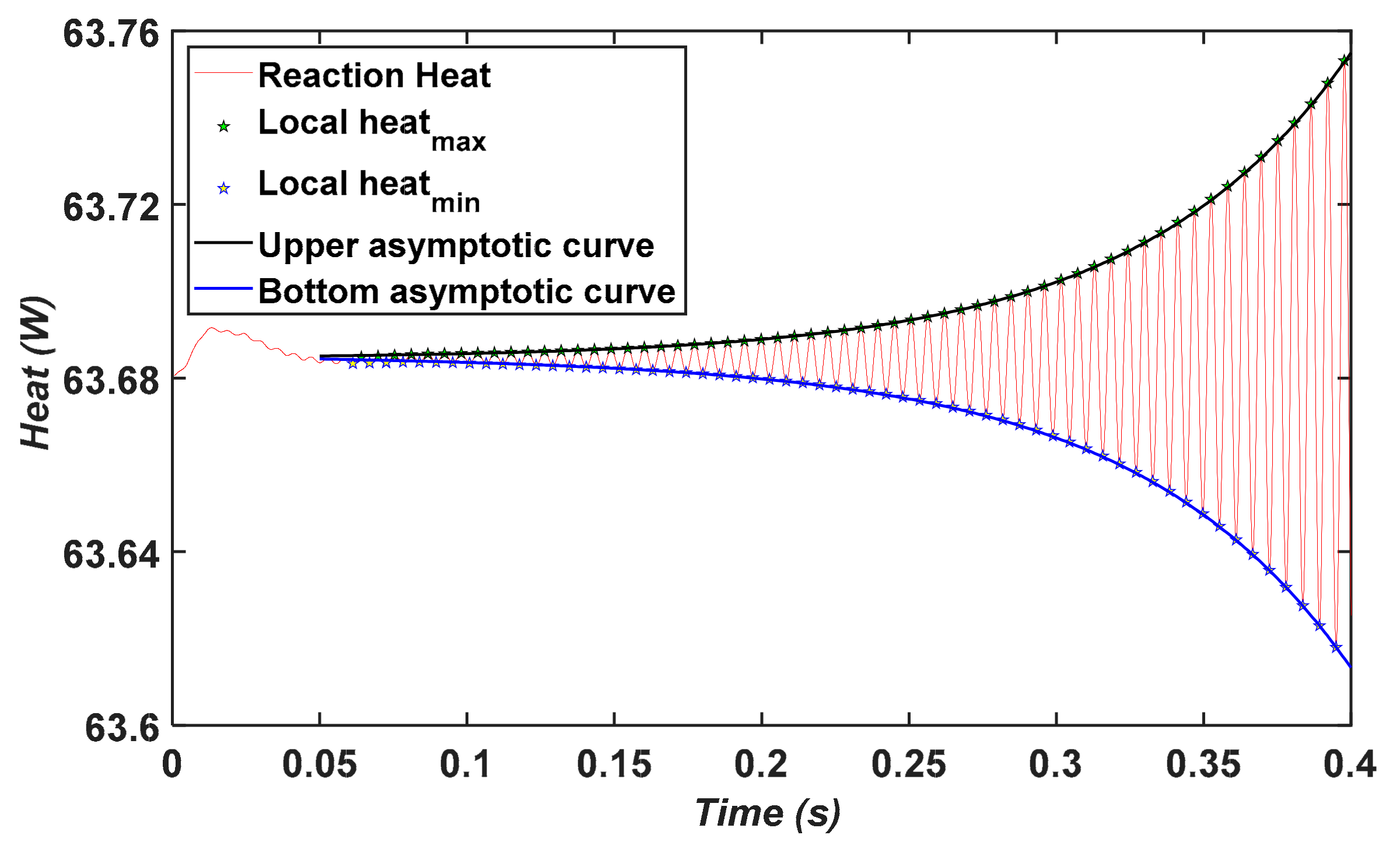
3.3. Self-Excited Pressure Oscillation—The Exponential Growth of Thermoacoustic Instability

To capture the dynamic characteristics of thermoacoustic insatiability, a transient simulation was conducted. Here, the steady-state reacting flow field was set as the initial condition of the dynamic flow. The time step was set to between $1\times {10}^{-5}\mathrm{s}$ and $1\times {10}^{-4}\mathrm{s}$ to obtain enough information in the time domain while meeting the convergent requirements in previous research [21,23,42]; here, it was set to $1\times {10}^{-5}$ s. The transient solution includes the growth of the self-excited instability, the subsequent limit cycle behavior of pressure and velocity, the oscillating frequencies and modes, and the periodic behavior of the flow field.

The instability growth mechanism is characterized by increasing oscillations of pressure inside the combustor. Figure 7a shows the time evolutions of average pressure and average velocity 5 cm downstream of the flame stabilizer. Figure 7b shows the growth of total reaction heat released by the flame. The steady-state value of pressure, velocity, and heat release were 0 Pa, 0.1226 m/s, and 63.68 W, respectively. Approximately 0.05 s after the time integration was initialized, the pressure, velocity, and reaction heat started to increase exponentially. The oscillation grew until approximately 0.86 s and reached maximum amplitudes. After several periods of amplitude adjustment from 0.86 s to 1.1 s, the system reached a “saturated” state, which is referred to as the limit cycle. The pressure, velocity, and reaction heat maintained at amplitudes of approximately 208 Pa, 0.39 m/s, and 10.79 W, respectively.

Figure 7d illustrated the phase relationship between the average pressure 5 cm downstream of the flame stabilizer and total heat release of the flame at the limit cycle oscillation state. The reaction heat release had a 24.3° phase delay relative to the pressure, which fulfills the Rayleigh criterion that oscillations are encouraged when heat fluctuates in phase with pressure perturbation [43]. It can be calculated that the reaction heat had a 114.34° phase delay relative to the velocity. This time delay between reaction heat and velocity has been proved to play a critical role in the stability of the Rijke-type thermoacoustic system [20].

Two important parameters to evaluate the growth of thermoacoustic instability are the growth rate of the acoustic disturbances α and G. The definition and detail derivation of α and G can be found in the reference [44]. The time evolution of the pressure and heat release of the flame from 0 s to 0.4 s are illustrated in Figure 8 and Figure 9. It can be seen that both the pressure and heat release were growing exponentially after an adjustment of about 0.05 s. Two exponential functions are constructed to best fit the series of local maximum and minimum points in Figure 8 and Figure 9, and they are written as:

$$\tilde{p}=\pm A{e}^{{\alpha }_{1}t}+B$$

(4)

$$\tilde{W}=\pm C{e}^{{\alpha }_{2}t}+D$$

(5)

where $\tilde{p}$ is the series of local maximum and minimum pressure, $\tilde{W}$ is the series of local maximum and minimum reaction heat, A, B, C, D, ${\alpha }_1$, ${\mathsf{\alpha }}_2$, and $\beta$ are parameters to be solved.

The Equations (4) and (5) are solved by iteration, and the calculated growth rate ${\alpha }_1$ is 13.77 ${\mathrm{s}}^{-1}$, ${\alpha }_2$is 13.85 ${\mathrm{s}}^{-1}$. The corresponding G is $1.22\times {10}^{-2}\mathrm{rad}/{\mathrm{s}}^2$, which is within the range of the maximum possible growth rate for this type of combustion-driven acoustic disturbance, $G_{max}$ = $9.2\times {10}^{-2}\mathrm{rad}/{\mathrm{s}}^2$.

From the analysis of Yoon et al. [18,19], the analytic pressure modes and velocity models of the acoustic perturbation for the acoustically closed–open Rijke-type burner can be expressed by Equations (6) and (7):

$$P_n=\cos (\left(2n-1\right)\mathsf{\pi }x/2\mathrm{L})n=1,2,3\cdots \infty$$

(6)

$$V_n=\sin (\left(2n-1\right)\mathsf{\pi }x/2\mathrm{L})n=1,2,3\cdots \infty$$

(7)

and the corresponding acoustic frequencies can be calculated by:

$$f_n=\frac{2n-1}{4L}an=1,2,3\cdots \infty .$$

(8)

where $f_n$ is the n-th acoustic frequency, and a is the sound speed.

According to the Rayleigh criterion, oscillations are encouraged when heat fluctuates in phase with pressure perturbation [43]. It can be determined from Equation (6) that the second acoustic mode may be excited when the unsteady heat is located at the center of the tube length because the flame is near the antinode of the second acoustic mode, which has a three-quarter wave mode shape. The frequency of this mode is 168.8 Hz with the inlet parameter by solving Equation (8).

The frequency component of the pressure oscillation from 1.4 s to 1.6 s is calculated and displayed in Figure 10. The excited frequency is 179 Hz, which is 6% higher than the predicted acoustic frequency of 168.8 Hz for the non-reacting flow. The small discrepancy is due to the flow in the tube being heated by the flame, which induced an increase in the sound speed. Furthermore, the increased sound speed resulted in an increase in the oscillation frequency. Thus, researchers should take the frequency increase effect into consideration when predicting the thermoacoustic instability frequency with the inlet parameters.

To compare the simulated oscillating mode with the prediction, the dynamic pressure along the centerline at time 1.400445 s was normalized by the maximum pressure amplitude, meanwhile the velocity along the center line at time 1.40585 s was normalized by the maximum velocity amplitude. In Figure 11, the normalized pressure and axial velocity of this work are compared with the analytical second acoustic pressure mode and velocity mode, and the normalized pressure and axial velocity in reference [23]. The simulation pressure distribution along the centerline is in good agreement with the analytical results and the results of Wang. While for the velocity distribution, two areas appear to have significant differences between the numerical results and the analytic results. The first area is in the flame stabilizer, where the simulated velocity is two times the analytical velocity because the flame stabilizer occupied half of the total volume of the entire flame stabilizer zone. The other inconsistent area is on the outlet face, because it was set as a pressure outlet, and the mass flow in the tube must be conserved. To further study this problem, it will be better to impose constraints on the velocity derivative on the outlet boundary. Aside from these two areas, the simulated velocity distribution agrees with the prediction results.

Figure 12 and Figure 13 show the instantaneous axial pressure distribution and axial velocity along the centerline of the Rijke burner at 8 different times of a limit cycle: namely, at times T, T/8, T/4, 3T/8, T/2, 5T/8, 3T/4, and 7T/8. In Figure 12, it can be seen that the pressure node point was at 1/3 length, and the pressure antinode point occurred downstream of the flame stabilizer at approximately 2/3 length, which matches the theoretical pressure maximum location for a three-quarter wave shown in Figure 11. From Figure 13, one can see that the velocity node point occurred slightly before the 2/3 tube length, which is also the pressure summit point of the pressure distribution.

3.4. Unsteady Flow Field in the Limit Cycle State

Figure 14 illustrates the axial velocity distribution and streamline at different times within a period of one limit cycle, where the yellow regions represent velocities above zero, the blue regions represent velocities below zero, and the gray regions represent the solid zone. Once the system is excited into the periodical oscillating state, the flow in the tube does not remain steady and uniform; rather, it begins oscillating back and forth. At the beginning of a period, the velocity was positive in the left 2/3 of the tube length and negative in the right 1/3 of the tube length, as shown in Figure 14a. At approximately 2/3 of the tube length, which is a node point of the velocity mode in the 1-D analysis, the axis velocity was zero. This result is in good agreement with the predicted velocity mode, and the velocity along the axis is in agreement with the velocity at time T in Figure 13. In the flame zone, due to the influence of the high-temperature flame, the flow was compressed and distorted, inducing the formation of a clockwise vortex after the flame area, as shown in Figure 14c. With the growth of this clockwise vortex, a counterclockwise vortex was formed at the inner wall of the left half of the tube in Figure 14d. These vortices were enlarged and changed the direction of flow in Figure 14e, making the flow negative on the left 2/3 of the tube length and positive on the right of the 1/3 tube length at time T+T/2, as shown in Figure 14f.

After time T+T/2, the flow was compressed near the inlet face and was expanded in the flame zone. When the negative flow was heated by the flame, followed by the formation of new vortices, and the subsequent development and collapse of these new vortices as shown in Figure 14g–j, the direction of flow changed in the opposite direction. A new period began.

The flow field variation in a limit cycle shown in Figure 14 demonstrates that vortices emerged and collapsed when thermoacoustic instability occurred. Thus, the computation of thermoacoustic instability should consider a turbulent flow, even in low Reynolds number cases.

Figure 15 and Figure 16 show the temperature distribution and kinetic rate of the reaction at T+T/2 and T+7/8T in a period, respectively. The distance between the flame and the flame stabilizer outlet was far in Figure 15a and Figure 16a, but close in Figure 15b and Figure 16b. In Figure 15a and Figure 16a, as time proceeds, the positive flow velocity moved the flame downstream, as shown in Figure 14c, and the flow before the 2/3 tube length was compressed to the maximum limit. Then, the pair of vortices broke down, and the flow was reversed, as shown in Figure 14d, where a vortex formed and the flow velocity decreased with time, causing the flow to become negative. The negative flow pushed the flame in the upstream direction, reaching the nearest point shown in Figure 15b and Figure 16b, at which time the flow in the left tube was compressed to the maximum limit, new separation points were generated, and new vortices changed the flow direction again, making the flame surface move downstream.

Thus, it can be concluded that the distance between the flame and flame stabilizer varies with the change in the axial velocity in the limit cycle state; the flow between the flame stabilizer and the 2/3 tube length is compressed when the axial velocity is positive, while it is expanded when the axial velocity is negative. During this periodic compression and expansion, the streamline is stretched and distorted, leading to the periodic formation and disappearance of vortices in the tube. This periodic behavior influences both the shape and distance of the flame via feedback; as a result, the forward feedback between the heat release and flow perturbation results in thermoacoustic instability.

4. Conclusions

A two-dimensional CFD simulation of a Rijke burner was conducted in this work. The self-excited thermoacoustic instability was numerically captured and analyzed, and the following conclusions are drawn.

• The onset and growth of the thermoacoustic instability were successfully captured. The simulated growth of the instability G was $1.22\times {10}^{-2}\mathrm{rad}/{\mathrm{s}}^2$, which is less than the maximum possible growth rate.
• The simulated oscillation frequency and mode were in good agreement with the 1-D analytical results. The simulated pressure oscillation frequency was 6% higher than the analytical results based on the inlet parameters, since the flow temperature and the sound speed were increased by the reaction heat. The normalized pressure and normalized velocity along the center line were in agreement with the prediction results of the second acoustic mode.
• As the system was excited into a limit cycle oscillation state, the amplitude of the velocity perturbation was larger than the average steady-state flow; thus, in some local areas, the flow velocity may be below zero, resulting in local backward flow in the burner.
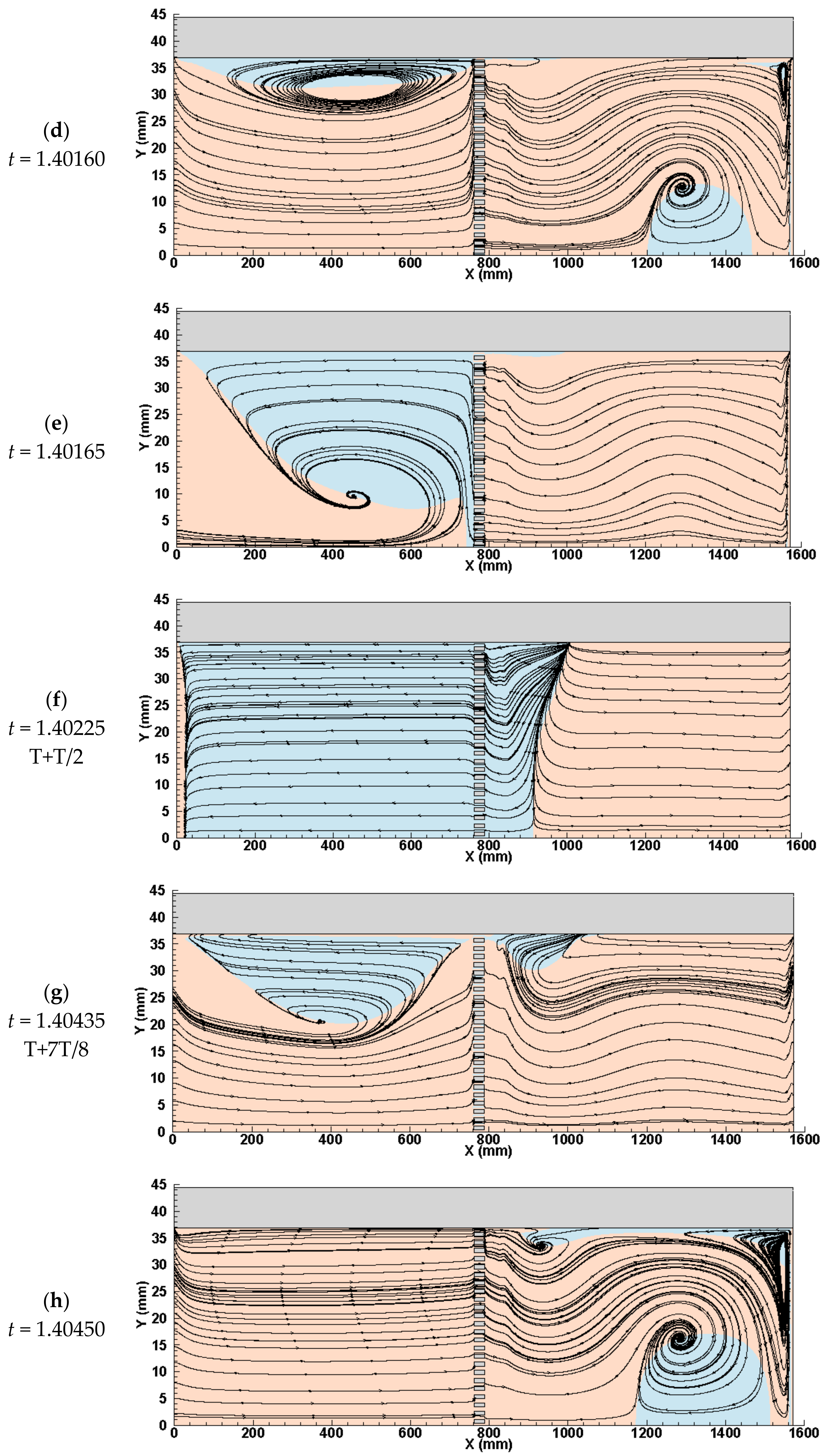
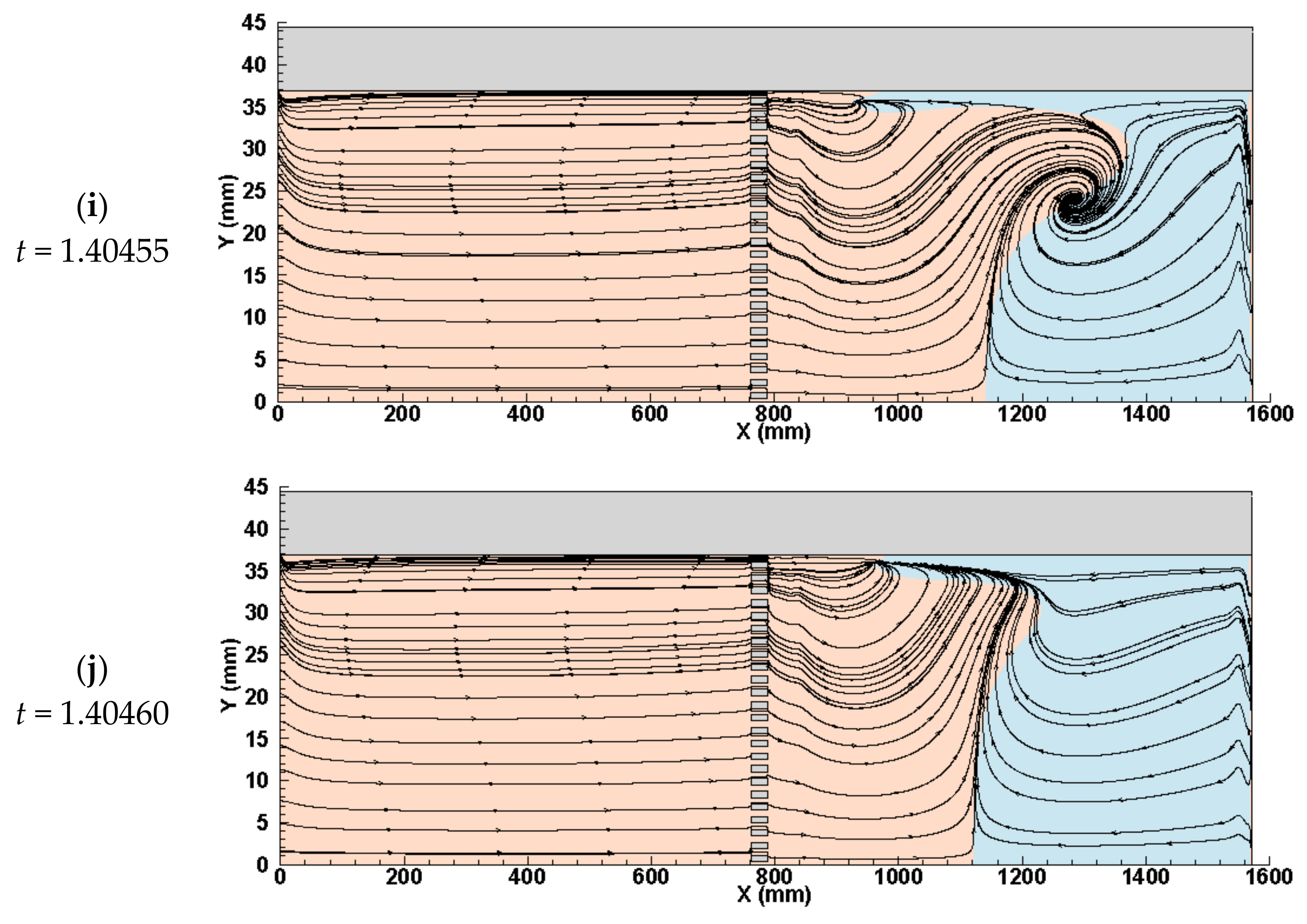
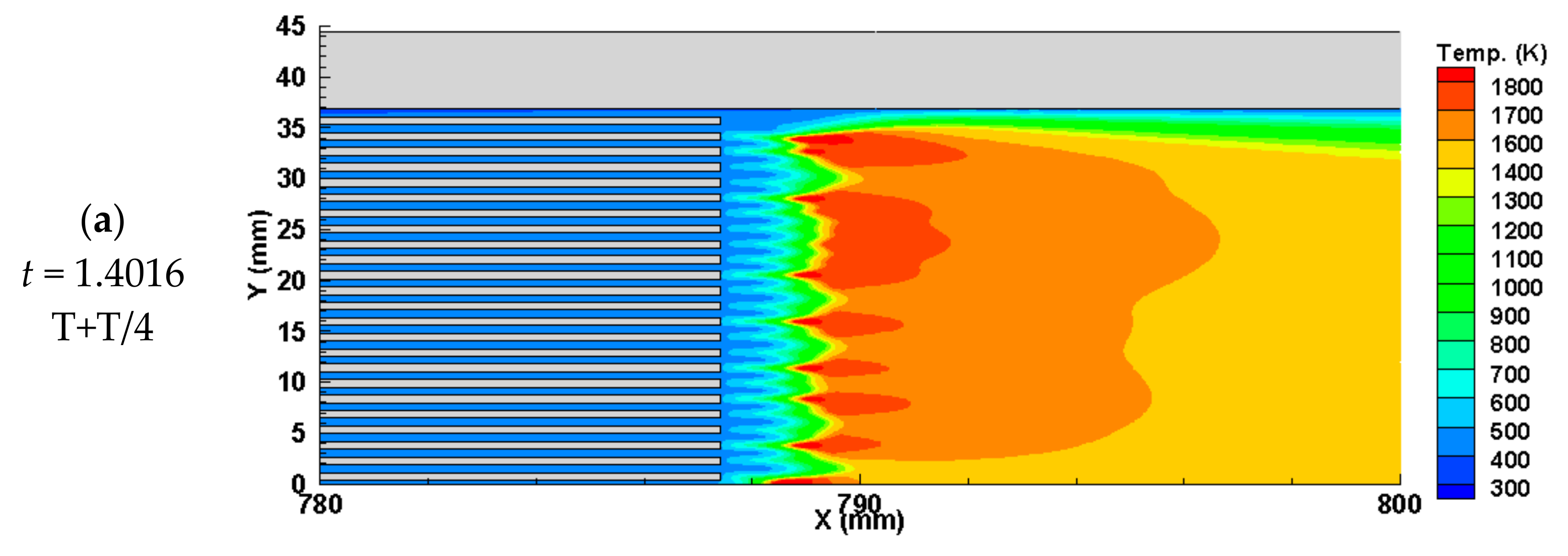
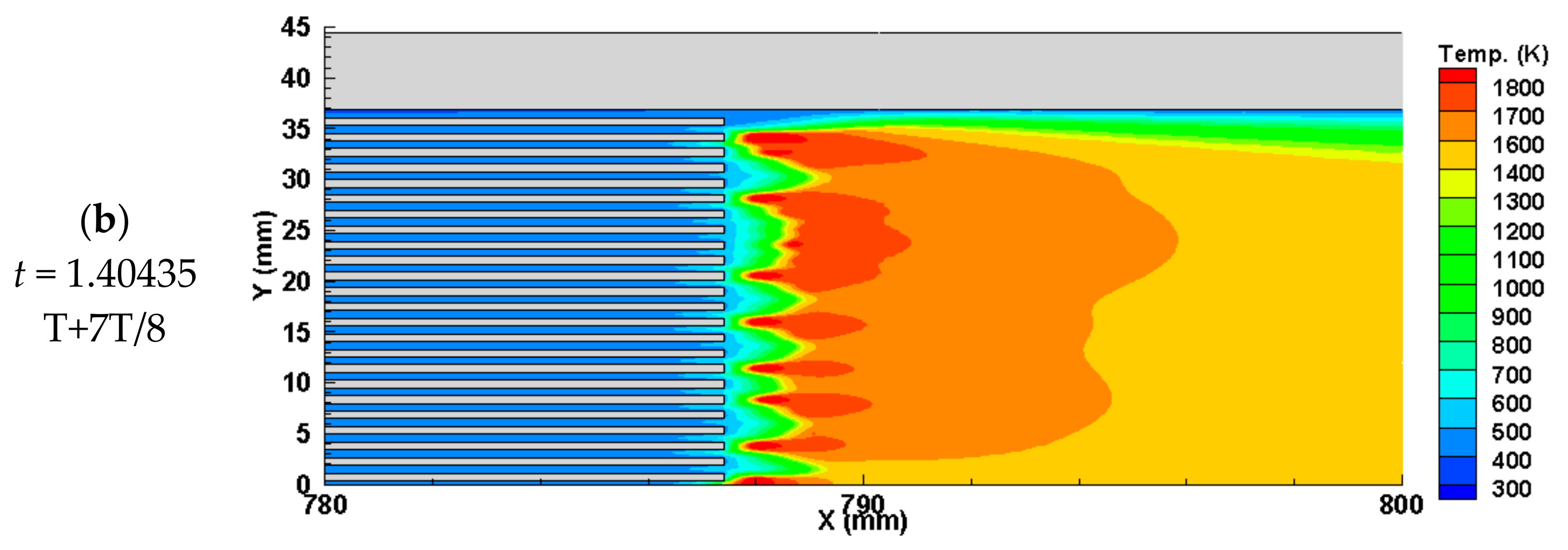
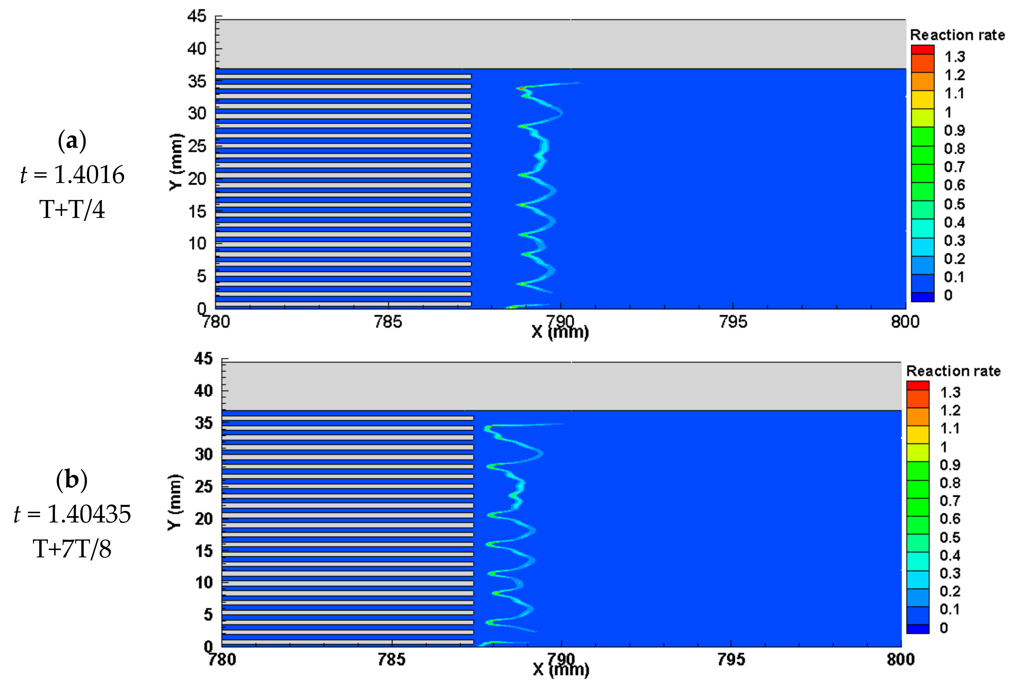
• In the limit cycle state, the distance between the flame and honeycomb outlet varied with the periodic change in the axial velocity. The flow between the flame stabilizer and the 2/3 tube length was periodically compressed and expanded, while the streamline was periodically stretched and distorted, inducing the periodic formation and disappearance of vortices in the tube. This is a typical behavior of flame-induced vortices, which leads to the flow field transition from laminar flow to turbulent flow.
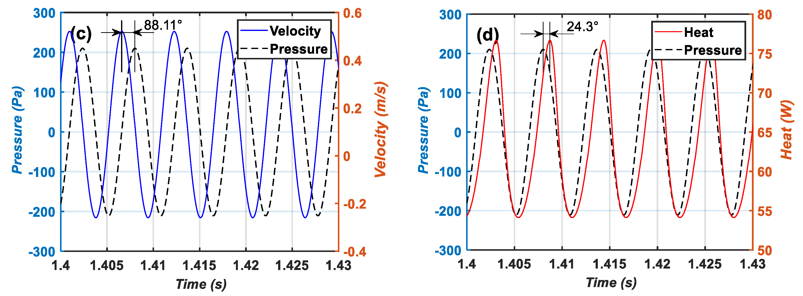
• The periodic behavior of the flow field induced by the unsteady heat release influenced both the shape and distance of the flame via feedback; thus, the forward interaction between the heat release and flow perturbation resulted in thermoacoustic instability.

References

1. Rijke, P.L. Notiz üoti eine neue Art, die in einer an beiden Enden offenen Röhre enthaltene Luft in Schwingungen zu versetzen. Ann. Phys. 1859, 183, 339–343. [Google Scholar] [CrossRef] [Green Version]
2. Raun, R.; Beckstead, M.; Finlinson, J.; Brooks, K. A review of Rijke tubes, Rijke burners and related devices. Prog. Energy Combust. Sci. 1993, 19, 313–364. [Google Scholar] [CrossRef]
3. Gotoda, H.; Nikimoto, H.; Miyano, T.; Tachibana, S. Dynamic properties of combustion instability in a lean premixed gas-turbine combustor. Chaos Interdiscip. J. Nonlinear Sci. 2011, 21, 013124. [Google Scholar] [CrossRef] [PubMed]
4. Kabiraj, L.; Sujith, R.I.; Wahi, P. Bifurcations of Self-Excited Ducted Laminar Premixed Flames. J. Eng. Gas Turbines Power 2011, 134, 031502. [Google Scholar] [CrossRef]
5. Zhao, D.; Chow, Z. Thermoacoustic instability of a laminar premixed flame in Rijke tube with a hydrodynamic region. J. Sound Vib. 2013, 332, 3419–3437. [Google Scholar] [CrossRef]
6. Weng, F.; Zhu, M.; Jing, L. Beat: A Nonlinear Thermoacoustic Instability in Rijke Burners. Int. J. Spray Combust. Dyn. 2014, 6, 247–266. [Google Scholar] [CrossRef]
7. Weng, F.; Li, S.; Zhong, D.; Zhu, M. Investigation of self-sustained beating oscillations in a Rijke burner. Combust. Flame 2016, 166, 181–191. [Google Scholar] [CrossRef]
8. Fleifil, M. Response of a laminar premixed flame to flow oscillations: A kinematic model and thermoacoustic instability results. Combust. Flame 1996, 106, 487–510. [Google Scholar] [CrossRef]
9. Dowling, A.P. A kinematic model of a ducted flame. J. Fluid Mech. 1999, 394, 51–72. [Google Scholar] [CrossRef]
10. Dowling, A.P. Nonlinear self-excited oscillations of a ducted flame. J. Fluid Mech. 1997, 346, 271–290. [Google Scholar] [CrossRef]
11. Zinn, B.T. A theoretical study of nonlinear combustion instability in liquid-propellant rocket engines. AIAA J. 1968, 6, 1966–1972. [Google Scholar] [CrossRef]
12. Zinn, B.T.; Lores, M.E. Application of the Galerkin Method in the Solution of Non-linear Axial Combustion Instability Problems in Liquid Rockets. Combust. Sci. Technol. 1971, 4, 269–278. [Google Scholar] [CrossRef]
13. Culick, F.E.C. Some recent results for nonlinear acoustics in combustion chambers. AIAA J. 1994, 32, 146–169. [Google Scholar] [CrossRef]
14. Culick, F. Nonlinear behavior of acoustic waves in combustion chambers—I. Acta Astronaut. 1976, 3, 715–734. [Google Scholar] [CrossRef]
15. Culick, F. Nonlinear behavior of acoustic waves in combustion chambers—II. Acta Astronaut. 1976, 3, 735–757. [Google Scholar] [CrossRef] [Green Version]
16. Culick, F.E.C.; Burnley, V.; Swenson, G. Pulsed instabilities in solid-propellant rockets. J. Propuls. Power 1995, 11, 657–665. [Google Scholar] [CrossRef]
17. Balasubramanian, K.; Sujith, R.I. Non-normality and nonlinearity in combustion–acoustic interaction in diffusion flames. J. Fluid Mech. 2007, 594, 29–57. [Google Scholar] [CrossRef]
18. Yoon, H.-G.; Peddieson, J.; Purdy, K.R. Mathematical modeling of a generalized Rijke tube. Int. J. Eng. Sci. 1998, 36, 1235–1264. [Google Scholar] [CrossRef]
19. Yoon, H.-G.; Peddieson, J.; Purdy, K.R. Non-linear response of a generalized Rijke tube. Int. J. Eng. Sci. 2001, 39, 1707–1723. [Google Scholar] [CrossRef]
20. Li, X.; Huang, Y.; Zhao, D.; Yang, W.; Yang, X.; Wen, H. Stability study of a nonlinear thermoacoustic combustor: Effects of time delay, acoustic loss and combustion-flow interaction index. Appl. Energy 2017, 199, 217–224. [Google Scholar] [CrossRef]
21. Chatterjee, P.; Vandsburger, U.; Saunders, W.R.; Khanna, V.K.; Baumann, W.T. On the spectral characteristics of a self-excited Rijke tube combustor—numerical simulation and experimental measurements. J. Sound Vib. 2005, 283, 573–588. [Google Scholar] [CrossRef]
22. Chatterjee, K.; Kumar, A.; Chatterjee, S.; Mukhopadhyay, A.; Sen, S. Numerical Simulation to Characterize Homogeneity of Air-Fuel Mixture for Premixed Combustion in Gas Turbine Combustor. In Proceedings of the ASME 2012 Gas Turbine India Conference, Mumbai, India, 1 December 2012; pp. 461–468. [Google Scholar]
23. Wang, Q.Z. Computational Investigations of Boundary Condition Effects on Simulations of Thermoacoustic Instabilities. Ph.D. Thesis, Virginia Polytechnic Institute and State University, Blacksburg, VA, USA, 2015. [Google Scholar]
24. Blanchard, R.; Ng, W.; Lowe, K.T.T.; Vandsburger, U. Simulating Bluff-Body Flameholders: On the Use of Proper Orthogonal Decomposition for Wake Dynamics Validation. J. Eng. Gas Turbines Power 2014, 136, 122603. [Google Scholar] [CrossRef]
25. Ghulam, M.M.; Gutmark, E.J. Computational Aeroacoustics for Analyzing Thermo-acoustic Instabilities in Afterburner Ducts. In Proceedings of the 2018 Joint Propulsion Conference, Cincinnati, OH, USA, 9–11 July 2018. [Google Scholar] [CrossRef]
26. Zhao, D.; Gutmark, E.; De Goey, P. A review of cavity-based trapped vortex, ultra-compact, high-g, inter-turbine combustors. Prog. Energy Combust. Sci. 2018, 66, 42–82. [Google Scholar] [CrossRef] [Green Version]
27. Markatos, N.C.; Cox, G. Hydrodynamics and heat transfer in enclosures containing a fire source. Physicochem. Hydrodyn. 1984, 5, 53–65. [Google Scholar]
28. Launder, B.; Spalding, D. The numerical computation of turbulent flows. Comput. Methods Appl. Mech. Eng. 1974, 3, 269–289. [Google Scholar] [CrossRef]
29. Zhao, D.; Guan, Y. Arne Reinecke.: Characterizing hydrogen-fuelled pulsating combustion on thermodynamic properties of a combustor. Commun. Phys. 2019, 2, 44. [Google Scholar] [CrossRef] [Green Version]
30. Li, Z.; Zhang, H. Numerical simulations of one-dimensional laminar premixed CH4/air flames using the detailed and one-step reaction mechanisms. J. Tsinghua. Univ. Sci. Tech. 2005, 45, 1510–1512. [Google Scholar] [CrossRef]
31. Acampora, L.; Marra, F.S.; Martelli, E. Comparison of Different CH4-Air Combustion Mechanisms in a Perfectly Stirred Reactor with Oscillating Residence Times Close to Extinction. Combust. Sci. Technol. 2016, 188, 707–718. [Google Scholar] [CrossRef]
32. Westbrook, C.K.; Dryer, F.L. Chemical kinetic modeling of hydrocarbon combustion. Prog. Energy Combust. Sci. 1984, 10, 1–57. [Google Scholar] [CrossRef]
33. Turns, S.R. An introduction to Combustion: Concepts and Applications; The McGraw-Hill Companies, Inc.: Singapore, 2000. [Google Scholar]
34. Abbud-Madrid, A.; Ronney, P.D. Effects of radiative and diffusive transport processes on premixed flames near flammability limits. Symp. Int. Combust. 1991, 23, 423–431. [Google Scholar] [CrossRef]
35. Howell, J.R.; Pinar, M.; Siegel, R. Thermal Radiation Heat Transfer; CRC Press: Boca Raton, FL, USA, 2015. [Google Scholar]
36. Ratzel, A.C.; Howell, J.R. Two-Dimensional Radiation in Absorbing-Emitting Media Using the P-N Approximation. J. Heat Transf. 1983, 105, 333–340. [Google Scholar] [CrossRef]
37. Cheng, P. Two-dimensional radiating gas flow by a moment method. AIAA J. 1964, 2, 1662–1664. [Google Scholar] [CrossRef]
38. Sazhin, S.; Sazhina, E.; Faltsi-Saravelou, O.; Wild, P. The P-1 model for thermal radiation transfer: Advantages and limitations. Fuel 1996, 75, 289–294. [Google Scholar] [CrossRef]
39. Krishnamoorthy, G. A computationally efficient P1 radiation model for modern combustion systems utilizing pre-conditioned conjugate gradient methods. Appl. Therm. Eng. 2017, 119, 197–206. [Google Scholar] [CrossRef] [Green Version]
40. Karyeyen, S. Combustion characteristics of a non-premixed methane flame in a generated burner under distributed combustion conditions: A numerical study. Fuel 2018, 230, 163–171. [Google Scholar] [CrossRef]
41. Kana-Donfack, P.; Kapseu, C.; Tcheukam-Toko, D.; Ndong-Essengue, G. Numerical Modeling of Sugarcane Bagasse Combustion in Sugar Mill Boiler. J. Energy Power Eng. 2019, 13, 80–90. [Google Scholar] [CrossRef]
42. Zhang, Y.; Wang, C.; Liu, X.; Che, D. Numerical study of the self-excited thermoacoustic vibrations occurring in combustion system. Appl. Therm. Eng. 2019, 160, 113994. [Google Scholar] [CrossRef]
43. Lord Rayleigh. The Theory of Sound, Vol.II; Dover: New York, NY, USA, 1945. [Google Scholar]
44. Zhao, D. Thermodynamics-Acoustics Coupling Studies on Self-Excited Combustion Oscillations Maximum Growth Rate. J. Therm. Sci. 2020, 1–13. [Google Scholar] [CrossRef]
Figure 1. Schematic of the Rijke burner and the honeycomb flame stabilizer (not to scale).
Applsci 11 01590 g001
Figure 2. Configuration of the axisymmetric Rijke burner model (not to scale).
Applsci 11 01590 g002
Figure 3. Comparison of the grid independence solutions of axial temperature.
Applsci 11 01590 g003
Figure 4. Reaction rate [kmol/m3·s] contour plots of the flame stabilizer channels and flame zone.
Applsci 11 01590 g004
Figure 5. Temperature contour plots of the flame stabilizer channels and flame zone.
Applsci 11 01590 g005
Figure 6. Species mass fraction distribution and reaction rate [kmol/m3·s] along the centerline.
Applsci 11 01590 g006
Figure 7. The time evolutions of pressure, velocity, and reaction heat release of the flame. (a) the time evolutions of pressure, velocity, (b) the time evolution of reaction heat release, (c) The phase relationship between velocity and pressure, and (d) the phase relationship between reaction heat release and pressure. Figure 7c illustrated the phase relationship between the average pressure and velocity 5 cm downstream of the flame stabilizer at the limit cycle oscillation state. It can be seen that the velocity had a 88.11° phase advance relative to the pressure.
Applsci 11 01590 g007aApplsci 11 01590 g007b
Figure 8. Time evolution of the pressure disturbances and the growth rate fitting curve.
Applsci 11 01590 g008
Figure 9. Time evolution of the unsteady heat release and the growth rate fitting curve.
Applsci 11 01590 g009
Figure 10. Fast Fourier transform (FFT) plot of the gauge pressure.
Applsci 11 01590 g010
Figure 11. Comparison of the simulated pressure and velocity along the centerline with the analytical prediction results.
Applsci 11 01590 g011
Figure 12. Pressure distribution along the centerline at different times of a limit cycle [Pa].
Applsci 11 01590 g012
Figure 13. Axial velocity distribution along the centerline at different times of a limit cycle [m/s].
Applsci 11 01590 g013
Figure 14. Axis velocity distribution in a cycle.
Applsci 11 01590 g014aApplsci 11 01590 g014bApplsci 11 01590 g014c
Figure 15. Temperature distribution at different times.
Applsci 11 01590 g015aApplsci 11 01590 g015b
Figure 16. Kinetic rate of reaction at different times.
Applsci 11 01590 g016
Publisher’s Note: MDPI stays neutral with regard to jurisdictional claims in published maps and institutional affiliations.