Inverse Kinematics Data Adaptation to Non-Standard Modular Robotic Arm Consisting of Unique Rotational Modules

Abstract

The paper describes the original robotic arm designed by our team kinematic design consisting of universal rotational modules (URM). The philosophy of modularity plays quite an important role when it comes to this mechanism since the individual modules will be the building blocks of the entire robotic arm. This is a serial kinematic chain with six degrees of freedom of unlimited rotation. It was modeled in three different environments to obtain the necessary visualizations, data, measurements, structural changes measurements and structural changes. In the environment of the CoppeliaSim Edu, it was constructed mainly to obtain the joints coordinates matching the description of a certain spatial trajectory with an option to test the software potential in future inverse task calculations. In Matlab, the model was constructed to check the mathematical equations in the area of kinematics, the model’s simulations of movements, and to test the numerical calculations of the inverse kinematics. Since the equipment at hand is subject to constant development, its model can also be found in SolidWorks. Thus, the model’s existence in those three environments has enabled us to compare the data and check the models’ structural designs. In Matlab and SolidWorks, we worked with the data imported on joints coordinates, necessitating overcoming certain problems related to calculations of the inverse kinematics. The objective was to compare the results, especially in terms of the position kinematics in Matlab and SolidWorks, provided the initial joint coordinate vector was the same.

1. Introduction

The paper addresses data processing (in particular those of joints coordinates, which are, in the case at hand, the angles of rotation) designated for a stationary robotic arm composed of the so-called URM modules, described in detail in [1,2,3]. We briefly mention their main attributes, which are unlimited rotation of the module around its own axis, availability of intrinsic power and modularity units. Thanks to the modularity and the advantages it represents [4,5,6,7], individual modules can be used for building various configurations and thus to adjust the arm to a function required of it, to create machines with different mobility capabilities, several degrees of freedom. In general, modular and reconfigurable robots offer great versatility, robustness and—thanks to their series production—low costs, which is mentioned by many authors addressing this issue [8,9,10]. Those modular, reconfigurable robots that consist of many modules (the number of their degrees of freedom is usually much greater than 6) have the ability to reconfigure themselves into a large number of shapes. If this is the case, the robot can change its shape to meet the requirements of different tasks.

Modular robotic systems are systems composed of modules that can be disconnected and reconnected in various configurations, subject to maintaining the precision and rigidity parameters, which can thus create a new system enabling new or value-added functions [11]. The concept of the URM system has been conceived in accordance with the total productive maintenance principal implementation rules [12,13]. Individual rotation positions are the result of the inverse kinematics of the mentioned robot’s arm. When it comes to kinematics of an inverse position, we look for such joint coordinate vectors of the open kinematic chain (assuming that the mechanism’s size is known) as would suit the required position and the orientation of the end effector’s coordinate system. Unlike the forward task, where the position vector is a function of the joint coordinate vector, the inverse task is substantially more complex because it necessitates solving a set of strongly nonlinear algebraic equations. These problems were first postulated by Paden B. [14] and Kahan W [15]. In most cases, these systems cannot be solved analytically. Thus, various types of iterative numerical methods are used, most often employing the Jacobian [16,17,18,19,20,21]. In calculating the inverse function, the inability to solve the task stems from the (configuration) workspace limitation, delimited by the configuration itself and the mechanism’s physical properties. If we are located outside this workspace, there is, of course, no solution. Several solutions may exist since the end effector’s defined position may be obtained in several manners. The situation can be even more varied in the case of the so-called redundant manipulators, where the joint coordinate vector’s number of elements is greater than the degree of freedom in the given workspace or plane. This results in an infinite number of configurations through which the defined position and orientation can be reached. We do not deal directly with the inverse function in this paper. The respective joint coordinates are obtained from the model’s CoppeliaSim Edu simulation (Coppelia Robotics AG, 8049 Zürich, Switzerland). The software calculating the inverse kinematics uses the pseudoinverse computational method, also called the Moore–Penrose method and the method of dampened least squares (DLS), also called the Levenberg–Marquardt method. More information about these and other methods can be found in [16,22,23,24]. Since other URM module configurations are contemplated for the future, or the redundant manipulator creation will be requested, it was mandatory to search for flexible solutions. To this end, the inverse kinematics is addressed in the CoppeliaSim Edu software. When the model is created in this environment, it enables the simulation of many types of movements and also the design of a working trajectory taking into account hurdles in the robotic arm’s configuration space. Joint coordinate vector coordinates are obtained from the model created in the CoppeliaSim Edu. Thus, we have the individual joints coordinates available, which is necessary for their subsequent implementation into the models, this time in Matlab (MathWorks, 1 Apple Hill Drive, Natick, MA 01760, USA) and in SolidWorks (Dassault Systèmes, 10 rue Marcel Dassault, CS 40501, 78946 Vélizy-Villacoublay CEDEX, France). These data are subsequently compared to check the models’ designs in the respective software environments. Should the designer’s work show ideal precision, these results should be, especially for the position kinematics, identical. This should hold regardless of the fact that two different software environments are used.

2. Model Creation and Data Processing

Relations describing the position kinematics by means of position vectors p_i, where iϵ<1;7> at individual open kinematic chain segments have also been derived in [25,26]. This is the case of the robotic arm’s forward kinematics. The relations serve the purpose of calculating the position of a point that would enable the attachment of either an effector or another device. Thus, the position of a point [p_xi, p_yi, p_zi] on the module will be defined by the function of the rotation positions φ_i, ϑ_i and the segment size of the structure at hand—|r_i|; p_i = f(φ_i, ϑ_i, r_i). The basis of the arm [1,2] is an autonomous, cylinder-shaped module. Such modules have a single degree of freedom, namely the rotational one. The rotation happens around the module’s main axis and is not limited in the interval under consideration ranging from 0 to 360 degrees. The rotation may occur continuously in either direction of rotation without limitation. The modules and joints are contemplated to be perfectly solid bodies. The individual modules’ axes of rotation cross each other at the point where they are joined by passive joints, Figure 1. The distances of section points in space are quantified by the r_i vector (a kinematic chain segment), and this vector has its own Cartesian system of S_i{O_i, x_i, y_i, z_i}. The segment’s rotation around the z_i axis is defined by the rotation matrix R_zi(φ_i) [3,4,5]. The segment’s rotation around the y_i axis is defined by the rotation matrix R_yi(ϑ_i).

Thus, we can write the following for R_zi(φ_i):

$${\mathit{R}}_{zi}\left({\phi }_i\right)=\left[\begin{array}{ccc}\cos \left({\phi }_i\right)& -\sin \left({\phi }_i\right)& 0\\ \sin \left({\phi }_i\right)& \cos \left({\phi }_i\right)& 0\\ 0& 0& 1\end{array}\right]$$

(1)

Moreover, the following for R_yi(ϑ_i):

$${\mathit{R}}_{yi}\left({\vartheta }_i\right)=\left[\begin{array}{ccc}\cos \left({\vartheta }_i\right)& 0& \sin \left({\vartheta }_i\right)\\ 0& 1& 0\\ -\sin \left({\vartheta }_i\right)& 0& \cos \left({\vartheta }_i\right)\end{array}\right]$$

(2)

The r₁ vector is connected to the base perpendicularly to the plane with the x₁, y₁ axes. p₁ ≡ r₁, because the coordinate system is orthogonal. According to Figure 1, the following applies to the position vector p₁:

$${\mathit{p}}_1={\mathit{R}}_{z1}\left({\phi }_1\right)\times {\mathit{r}}_1$$

(3)

According to Figure 1, the following applies to the position vectors p₂, p₃, p₄, to p_i:

$${\mathit{p}}_2={\mathit{p}}_1+{\mathit{R}}_{z1}\left({\phi }_1\right)\times {\mathit{R}}_{y2}\left({\vartheta }_2\right)\times {\mathit{R}}_{z2}\left({\phi }_2\right)\times {\mathit{r}}_2$$

(4)

$${\mathit{p}}_3={\mathit{p}}_2+{\mathit{R}}_{z1}\left({\phi }_1\right)\times {\mathit{R}}_{y2}\left({\vartheta }_2\right)\times {\mathit{R}}_{z2}\left({\phi }_2\right)\times {\mathit{R}}_{y3}\left({\vartheta }_3\right)\times {\mathit{R}}_{z3}\left({\phi }_3\right)\times {\mathit{r}}_3$$

(5)

$${\mathit{p}}_4={\mathit{p}}_3+{\mathit{R}}_{z1}\left({\phi }_1\right)\times {\mathit{R}}_{y2}\left({\vartheta }_2\right)\times {\mathit{R}}_{z2}\left({\phi }_2\right)\times {\mathit{R}}_{y3}\left({\vartheta }_3\right)\times {\mathit{R}}_{z3}\left({\phi }_3\right)\times {\mathit{R}}_{y4}\left({\vartheta }_4\right)\times {\mathit{R}}_{z4}\left({\phi }_4\right)\times {\mathit{r}}_4$$

(6)

A general position vector formula of this p_i structure will thus be:

$${\mathit{p}}_{i+1}={\mathit{R}}_{z1}\left({\phi }_1\right)\times \left[{\mathit{r}}_1+{\displaystyle \sum }_{k=1}^i\left[{\displaystyle \prod }_{j=1}^k\left({\mathit{R}}_{y\left(j+1\right)}\left({\vartheta }_{j+1}\right)\times {\mathit{R}}_{z\left(j+1\right)}\left({\phi }_{j+1}\right)\right)\right]\times {\mathit{r}}_{k+1}\right]$$

(7)

The resulting orientation of the r_i vector defined by the Euler’s angle can be seen in [27] according to the R_z(γ)R_y(β)R_x(α) option will be determined from the relation below based on the final arm rotation:

$${\mathit{R}}_{ZYX\left(i+1\right)}={\mathit{R}}_{z1}\left({\phi }_1\right)\times {\displaystyle \prod }_{j=1}^i\left({\mathit{R}}_{y\left(j+1\right)}\left({\vartheta }_{j+1}\right)\times {\mathit{R}}_{z\left(j+1\right)}\left({\phi }_{j+1}\right)\right)$$

(8)

Generally speaking, the final shape of the R_ZYX(i+1) in terms of its i-segment will look as follows:

$${\mathit{R}}_{ZYX\left(i+1\right)}=\left[\begin{array}{ccc}{\mathrm{a}}_{11}& {\mathrm{a}}_{12}& {\mathrm{a}}_{13}\\ {\mathrm{a}}_{21}& {\mathrm{a}}_{22}& {\mathrm{a}}_{23}\\ {\mathrm{a}}_{31}& {\mathrm{a}}_{32}& {\mathrm{a}}_{33}\end{array}\right]$$

(9)

where a_ij for i = 1, 2, 3, j = 1, 2, 3 are the matrix elements. Considering the R_z(γ)R_y(β)R_x(α) option, the Euler’s angles will then be as follows:

$$\alpha =\arctan \left(\frac{{\mathrm{a}}_{32}}{{\mathrm{a}}_{33}}\right)$$

(10)

$$\beta =\arcsin \left(-{\mathrm{a}}_{31}\right)$$

(11)

or also:

$$\beta =\arctan \left(\frac{-{\mathrm{a}}_{31}}{\sqrt{{\mathrm{a}}_{32}^2+{\mathrm{a}}_{33}^2}}\right)$$

(12)

$$\gamma =\arctan \left(\frac{{\mathrm{a}}_{21}}{{\mathrm{a}}_{11}}\right)$$

(13)

Thus, for example, in the case of an arm with 3 active degrees of freedom, i.e., for the r₄ vector, the final rotation according to Equation (8) will be as follows:

$${\mathit{R}}_{ZYX4}={\mathit{R}}_{z1}\left({\phi }_1\right)\times {\mathit{R}}_{y2}\left({\vartheta }_2\right)\times {\mathit{R}}_{z2}\left({\phi }_2\right)\times {\mathit{R}}_{y3}\left({\vartheta }_3\right)\times {\mathit{R}}_{z3}\left({\phi }_3\right)\times {\mathit{R}}_{y4}\left({\vartheta }_4\right)$$

(14)

Our case involves 6 degrees of freedom.

2.1. Modeling in CoppeliaSim Edu

An open kinematic chain model was created in CoppeliaSim Edu, in Figure 2, composed of modules featuring 6 degrees of freedom.

The purpose of this model was especially calculating the inverse task from an arbitrary spatial trajectory the effector is to travel under 37 s. Joint coordinate vector data φ = [φ₁, φ₂, …, φ₆]^T are obtained using a sampling period of T_sp each 0.005 s. The only (software-imposed) limitation is the degree of freedom itself, namely the possibility of rotation in the <−π, +π> interval. This problem had to be subsequently addressed since it was causing a discontinuity in the simulation’s operation as per the condition (18) and was thus disrupting the continuity of the trajectory on the models in the environments into which data were imported., i.e., Matlab, SolidWorks, but the same would have been the case in other environments, too.

2.2. Modeling in Matlab

The kinematic model in Figure 3 was created in Matlab using the Simscape/Multibody toolbox, the dimensions of which reflect the reality and are given in

Table 1. Dimensions table of the robotic arm of Figure 2 and also Figure 3, Figure 4, respectively.

Diameters	(mm)	Diameters	(mm)	Diameters	(mm)
r1	243.215	a1	73	b1	128
r2	212.430	a2	42.215	b2	128
r3	212.430	a3	42.215	b3	128
r4	212.430	a4	42.215	b4	128
r5	212.430	a5	42.215	b5	128
r6	212.430	a6	42.215	b6	128
r7	42.215 1

¹ Effector (last part of the passive joint).

. The module diameter or volume need not be of interest when making a kinematic assessment, as it has no effect on kinematic parameters.

The model is composed of individual blocks that define its parts. In a nutshell, the model consists of a base identical to the “base” of the reference system and the individual blocks representing the r_i vector (a kinematic chain segment). As we can see in Figure 1, the “vector r _I” block then consists of the “URM“ module and a passive joint part. The modules are connected in places where each joint represents its own Cartesian system of the module, starting in point O_i. In this experiment, the last part of the passive joint, vector r₇, was considered to be an effector. A measuring device (sensor 7) is connected to the effector r₇, checking physical quantities (position, velocity, acceleration). Such measuring devices can be mounted on other modules, too. The Euler’s angles’ values are also available in three consecutive rotations around the axes, often marked ZYX. The values apply to the effector and are the result of the final product of the individual spatial transformations (8), as is usually the case with the open kinematic chain [27]. A model constructed in this way is then visualized in the Mechanics explorer window and appears in the form as seen in Figure 4.

2.3. The Problem of a Sudden Change in Data Continuity and Its Solution in Matlab

The task was to use the computational core of CoppeliaSim Edu and apply it to the inverse kinematic task, to calculate the joint coordinates of φ = [φ₁, φ₂, …, φ₆]^T for the entered trajectory. When the joint coordinates data were imported, in some cases, the above-mentioned problem with value repolarization emerged as a result of the software-imposed limitation on the joint rotation. In other words, in the case of a requirement arising from the calculation, the range of the degree of freedom upon exceeding the rotation values in the <−π, +π> interval must be switched to the value with the opposite sign to remain in the defined working interval. The values above the upper limit +π will rise again, but this time starting with the lower value of −π. Moreover, the opposite values below the lower limit −π will fall again, this time starting from the upper value of +π. This sudden change causes deformation or even computational instability of the p₇ trajectory of the effector, see Figure 5. With time derivations of the position, the characteristics of instantaneous velocity and accelerations are deformed even more.

Since the precision of the trajectory traveled by any manipulator is critical in practical applications, it was necessary to somehow address this problem. Either through a labor-intensive rewriting of the imported data upon each change in the defined trajectory subject to the presence of those repolarizations in the joints or through a suitable solution. One such solution is the so-called repolarize, described below.

2.4. Composing a Repolarize

The search for a suitable and undemanding solution to this situation rested on the following conditions:

• To maintain the original trajectory, the initial values should not be skewed, i.e., if possible, they should not be averaged or approximated;
• There should be no phase shift of the initial values, as is the case with many filters.

For these reasons, we were trying to apply different approaches in the simulation, starting with a change in the initial data φ = [φ₁, φ₂, φ₃, φ₄, φ₅, φ₆]^T, which was very labor-intensive. The rate limiter has not met the expectations either [28] in switching the data flow at the moment of reaching the limits of the angles of rotation +/−π, because the characteristics of the p₇ trajectory were undulated anyway. Rate limiter is a marginalized derivation of an infinitely small difference to a difference of finite size. Or similar approaches based on a sequential omission of the undesired sample, such as in [29]. Or through averaging the values [30,31]. Neither of the approaches mentioned in this case has met our expectations. The best, if not ideal, results were finally achieved by the system working on this principle Figure 6 and explained in Figure 7. Joint coordinate data were measured in the sampling period T_sp every 0.005 s.

When the data were uploaded, it was first necessary to establish the moment of repolarization t_r with the precision of δ = +/−0.0025 s when the variable φ(t) = 0, i.e., cuts through the time axis. Under the assumption of reaching the upper or the lower working interval limit <−π, +π> of the joint coordinate. The variable at the output from the repolarize is φ_out(t). It was necessary to meet the following conditions:

$$t\le t_1|{\phi }_{out}\left(t\right)=\phi \left(t\right)$$

(15)

$$t_1<t_2$$

(16)

Conditions for identification of the sign and carrying out repolarization over time t_r:

$$t\ge t_2|{\phi }_{out}\left(t\right)=\{\begin{array}{c}2\pi -\phi \left(t\right), \phi \left(t\right)<0\\ \phi \left(t\right)-2\pi , \phi \left(t\right)>0\end{array}$$

(17)

For the condition that can be considered discontinuation in the angle variable data φ(t), the following applies:

$$\frac{\left|\phi \left(t+T_{sp}\right)-\phi \left(t\right)\right|}{T_{sp}}=\frac{2\pi }{T_{sp}}$$

(18)

The model was thus “excited” by the values of the joint coordinate vector φ(t) = [φ₁(t), φ₂(t), …, φ_n(t)]^T obtained from the model created in CoppeliaSim Edu in the period of time T_sp. Under the condition of the prescribed maximum permissible deviation [Δ_{max x}, Δ_{max y}, Δ_{max z}] = +/−0.0035 m between the real trajectory and the one calculated on the basis of inverse kinematics. The data of joint coordinates φ(t) correspond to the effectors of the trajectory traveled. The trajectory is made of a system of fixed points A_s{x_As, y_As, z_As}, where the sample sϵ<1; 7383> in Cartesian space Figure 8. Its real shape is shown in Figure 2.

The mutual calibration of the models was done for the initial position of the robotic arm effector over time t = 0 s, φ(0) = [0, π, 0, π, 0, π]^T radians see position in Figure 4, p₇ = [0.167397, 0, 1.102644]^T meters. In order to check the models’ correctness, the vector difference Δ = [Δ_x, Δ_y, Δ_z]^T between the position of the position vector effector p₇ = [p_7x, p_7y, p_7z]^T and the position of the A_s points, composing the trajectory, shown in the graph of Figure 9 (Matlab), Figure 12 (SolidWorks) over the period of time T_sp. This was done for each vector component. The following applies to Δ vector components, its norm ‖Δ‖ and the instantaneous time t of the sample in seconds:

$${\Delta }_x=x_{As}-p_{7x}\left(\mathit{\phi }\right)$$

(19)

$${\Delta }_y=y_{As}-p_{7y}\left(\mathit{\phi }\right)$$

(20)

$${\Delta }_z=z_{As}-p_{7z}\left(\mathit{\phi }\right)$$

(21)

$$t=0.005\left(s-1\right)|s\in \langle 1;7383\rangle$$

(22)

$$\Vert \mathbf{\Delta }\Vert =\sqrt{{\Delta }_x{}^2+{\Delta }_y{}^2+{\Delta }_z{}^2}$$

(23)

As we can see, the CoppeliaSim Edu software complied with the tolerance range requirement +/− 0.0035 m for each vector component, for the inverse calculation of the joint coordinate data φ(t) with respect to the trajectory consisting of a finite set of A_s points. The characteristics of physical quantities from sensor 7 in the model see Figure 3 (position, velocity, acceleration) are shown in Figure 10. We note that this is a different data set (different trajectory) than the one used in the illustration of Figure 5.

2.5. Modeling in SolidWorks

In order to carry out structural changes, various structural compositions of the robotic arm composed of the URM modules are created in SolidWorks are shown in Figure 11. This mechanically detailed model corresponding to the reality was in the same dimensional configuration Table 1, as was used for making a comparison of kinematic indices and also the Δ_x, Δ_y, Δ_z difference between the real and the calculated trajectory.

In this case, too, the graph of Figure 12 has confirmed that the requirement for a tolerance range of +/−0.0035 m for each vector component was adhered to by the inverse calculation of the joint coordinate data φ(t) with respect to the trajectory composed of a finite set of the A_s points.

Here, however, certain changes in the shape of the course can be observed, which is logical, as we are dealing with two different software environments and the model structure itself as well. The norm, i.e., the size of the vector of deviation from the original trajectory ‖Δ‖ already has a permanent value of 0.0025 m here, and no significant minima can be seen in the three places where the trajectory “breaks” see Figure 2. The characteristics of physical quantities corresponding to the effector in the model see Figure 11 (position, velocity) are illustrated in Figure 13.

As we can see, the characteristics of position and velocity alike Figure 13a,b, corresponding to the effector in the model of Figure 11, are similar to the characteristics shown in Figure 10a,b.

3. Results

The robotic arm model was created in CoppeliaSim Edu in order to obtain the joints coordinates, corresponding to a description of the spatial trajectory consisting of the fixed points A_s{x_As, y_As, z_As} with a permissible deviation of +/−0.0035 m from the original trajectory.

Results obtained in Matlab are shown in Figure 9 and Figure 10. Figure 9 shows the difference Δ_x, Δ_y, Δ_z between the real trajectory (consisting of the A_s{x_As, y_As, z_As} points) and the one calculated (from the components of the position vector effector p_7x, p_7y, p_7z). On the other hand, Figure 10 shows the values measured on the effector, namely:

(a)

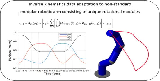
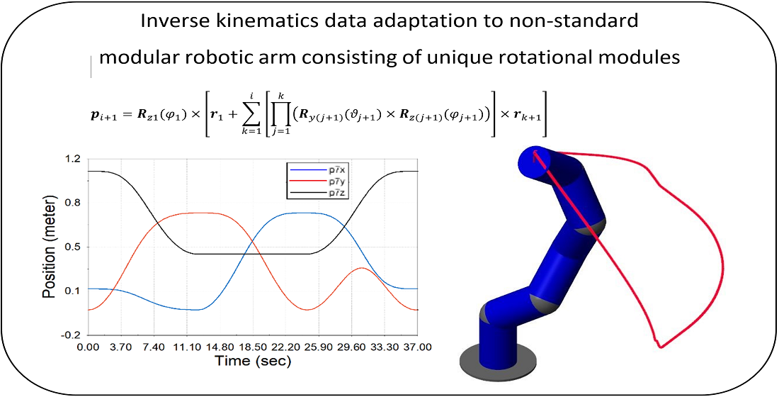
The position determined by the position vector p₇ = [p_7x, p_7y, p_7z]^T depending on the joint coordinate vector φ(t);

(b)

The speed determined by the velocity vector v₇ = [v_7x, v_7y, v_7z]^T depending on the first derivation (time-bound) of the joint coordinate vector φ′(t);

(c)

The acceleration determined by the acceleration vector a₇ = [a_7x, a_7y, a_7z]^T depending on the second derivation (time-bound) of the joint coordinate vector φ″(t) and (φ′(t))²;

(d)

The orientation determined by the Euler’s angles according to the [γ, β, α] option, depending on the joint coordinate vector φ(t).

Figure 5 shows the importance of using the repolarize. Otherwise, the joint coordinate data must be edited manually prior to their import, as was the case with SolidWorks.

The results obtained in SolidWorks are shown in Figure 12 and Figure 13. Figure 12 shows the Δ_x, Δ_y, Δ_z difference between the real trajectory (consisting of the A_s{x_As, y_As, z_As} points) and the one calculated (from the position vector effector components of p_7x, p_7y, p_7z). On the other hand, Figure 13 shows the values generated on the effector, namely:

(a)

The position determined by the position vector p₇ = [p_7x, p_7y, p_7z]^T depending on the joint coordinate vector φ(t);

(b)

The speed determined by the velocity vector v₇ = [v_7x, v_7y, v_7z]^T depending on the first derivation (time-bound) joint coordinate vector φ′(t).

4. Discussion

Based on the above results, we can conclude that the currently available software environments offer not only relatively powerful visualization tools but also those enabling various kinds of physical computations. The quality of results depends not only on the sophistication of the software and its preferable use but also on correct parameter specification, on the defined conditions and on the application of the software to its maximum potential. The aim of our work was especially to enable the comparison of data from the position kinematics in Matlab and in SolidWorks, subject to the same initial joint coordinate vector φ(t). This has enabled us to check the designed models and to detect eventual structural discrepancies such as counter-rotation of the URM module or an undesirable shift of structural elements.

Matlab made it possible to choose the manner of processing the imported data, to align the sampling step with the CopeliaSim imported data step and thus ensure that a particular input datum actually corresponded to the given output value over the same time. It was possible to additionally construct a system to accommodate some changes in the input data Figure 6 and thus to make the work involved in input data changes more effective. The difference between the real and the calculated trajectory was quantified using the Δ vector. Figure 9b shows that the vector size ‖Δ‖ reaches its maxima at the maximum effector velocities.

In SolidWorks, the difference between the real and the calculated trajectory Δ was already different in nature; see Figure 12. Here, the ‖Δ‖ vector size has a permanent value and changes only slightly; no significant minima are observed here in the places where the trajectory “breaks”, as shown in Figure 2.

References

- Svetlík, J.; Štofa, M.; Pituk, M. Prototype development of a unique serial kinematic structure of modular configuration. MM Sci. J. 2016, 994–998. [Google Scholar] [CrossRef]
- Svetlík, J. Contribution to Construction of Manufacturing Engineering on Flexible Architecture Basis. Habilitation Thesis, Technical University of Košice, Košice, Slovakia, 14 June 2012. [Google Scholar]
- Štofa, M. Experimentálny vývoj rotačných modulov pre stavbu sériových kinematických štruktúr vo výrobnej technike. Ph.D. Thesis, Technical University of Košice, Košice, Slovakia, 30 January 2020. [Google Scholar]
- Gershenson, J.K.; Prasad, G.J. Modularity in product design for manufacturability. Int. J. Agile Manuf. 1997, 3, 99–110. [Google Scholar]
- Benderbal, H.H.; Dahane, M.; Benyoucef, L. Modularity assessment in reconfigurable manufacturing system (RMS) design: An Archived Multi-Objective Simulated Annealing-based approach. Int. J. Adv. Manuf. Technol. 2018, 94, 729–749. [Google Scholar] [CrossRef]
- Pérez, R.; Aca, J.; Valverde, A. A modularity framework for concurrent design of reconfigurable machine tools. In Proceedings of the International Conference on Cooperative Design, Visualization and Engineering, Heidelberg, Germany, 19–22 September 2004; Springer: Berlin, Germany, 2004. [Google Scholar]
- Svetlík, J. Modularity of Production Systems. In Machine Tools; Šooš, Ľ., Marek, J., Eds.; IntechOpen: London, UK, 2020; pp. 1–22. [Google Scholar]
- Yim, M.; Duff, D.G.; Roufas, K.D. PolyBot: A modular reconfigurable robot. In Proceedings of the ICRA ’00, IEEE International Conference on Robotics and Automation, San Francisco, CA, USA, 24–28 April 2000; Volume 1, pp. 514–520. [Google Scholar]
- Yim, M.; Roufas, K.; Duff, D.; Zhang, Y.; Eldershaw, C.; Homans, S. Modular reconfigurable robots in space applications. Auton. Robot. 2003, 14, 225–237. [Google Scholar] [CrossRef]
- Acaccia, G.; Bruzzone, L.; Razzoli, R. A modular robotic system for industrial applications. Assem. Autom. 2008, 28, 151–162. [Google Scholar] [CrossRef]
- Xu, W.; Han, L.; Wang, X.; Yuan, H. A wireless reconfigurable modular manipulator and its control system. Mechatron. 2021, 73, 102470. [Google Scholar] [CrossRef]
- Pacaiova, H.; Isiarikova, G. Base Principles and Practices for Implementation of Total Productive Maintenance in Automotive Industry. Qual. Innov. Prosper. 2019, 23, 45–59. [Google Scholar] [CrossRef]
- Nikitin, Y.; Bozek, P.; Peterka, J. Logical–linguistic model of diagnostics of electric drives with sensors support. Sensors 2020, 20, 4429. [Google Scholar] [CrossRef] [PubMed]
- Paden, B. Kinematics and Control Robot Manipulators. Ph.D. Thesis, University of California, Berkeley, CA, USA, 1986. [Google Scholar]
- Kahan, W. Lectures on Computational Aspects of Geometry; Department of Electrical Engineering and Computer Sciences, University of California: Berkeley, CA, USA, 1983; Unpublished. [Google Scholar]
- Buss, S.R. Introduction to inverse kinematics with jacobian transpose, pseudoinverse and damped least squares methods. IEEE J. Robot. Autom. 2004, 16, 1–19. [Google Scholar]
- Dulęba, I.; Opałka, M. A comparison of Jacobian-based methods of inverse kinematics for serial robot manipulators. Int. J. Appl. Math. Comput. Sci. 2013, 23, 373–382. [Google Scholar] [CrossRef]
- Meredith, M.; Maddock, S. Real-Time Inverse Kinematics: The Return of the Jacobian; Technical Report No. CS-04-06; Department of Computer Science, University of Sheffield: Sheffield, UK, 2004. [Google Scholar]
- Šoch, M.; Lórencz, R. Solving inverse kinematics—A new approach to the extended Jacobian technique. Acta Polytech. 2005, 45, 21–26. [Google Scholar]
- Virgala, I.; Gmiterko, A.; Surovec, R.; Vacková, M.; Prada, E.; Kenderová, M. Manipulator end-effector position control. Procedia Eng. 2012, 48, 684–692. [Google Scholar] [CrossRef][Green Version]
- Virgala, I.; Tomáš, L.; Miková, Ľ. Snake robot locomotion patterns for straight and curved pipe. J. Mech. Eng. 2018, 68, 91–104. [Google Scholar] [CrossRef]
- Nilsson, R. Inverse Kinematics. Master’s Thesis, Luleå University of Technology, Luleå, Sweden, 2009. [Google Scholar]
- Wampler, C.W. Manipulator inverse kinematic solutions based on vector formulations and damped least-squares methods. IEEE Trans. Syst. Man, Cybern. 1986, 16, 93–101. [Google Scholar] [CrossRef]
- Lozhkin, A.; Bozek, P.; Maiorov, K. The method of high accuracy calculation of robot trajectory for the complex curves. Manag. Syst. Prod. Eng. 2020, 28, 247–252. [Google Scholar] [CrossRef]
- Ondočko, Š.; Stejskal, T.; Svetlík, J.; Hrivniak, L.; Šašala, L. Direct kinematics of modular system. In Automatizácia a riadenie v teórii a praxi 2020, Proceedings of the 14. ročník konferencie odborníkov z univerzít, vysokých škôl a praxe, Stará Lesná, Slovensko, 5–7 February 2020; Šeminský, J., Mižáková, J., Šimšík, J., Balog, M., Eds.; Technická Univerzita v Košiciach: Košice, Slovakia, 2020. [Google Scholar]
- Ondočko, Š.; Stejskal, T.; Svetlík, J.; Hrivniak, L.; Šašala, L.; Žilinský, A. Position forward kinematics of 6-DOF robotic arm. Acta Mech. Slovaca. (under review).
- Murray, R.; Li, Z.; Shankar, S. A Mathematical Introduction to Robotic Manipulation, 1st ed.; CRC Press: Boca Raton, FL, USA, 2017; p. 519. ISBN 9781315136370. [Google Scholar]
- Rate Limiter. Available online: https://www.mathworks.com/help/simulink/slref/ratelimiter.html?s_tid=srchtitle (accessed on 29 October 2020).
- How to Remove Unwanted Short Time Signal Simulink. Available online: https://stackoverflow.com/questions/52384093/how-to-remove-unwanted-short-time-signal-simulink/52409614 (accessed on 29 October 2020).
- Filtering and Smoothing Data. Available online: https://www.mathworks.com/help/curvefit/smoothing-data.html (accessed on 29 October 2020).
- Signal Smoothing. Available online: https://www.mathworks.com/help/signal/ug/signal-smoothing.html (accessed on 29 October 2020).