Building a Realistic Virtual Simulator for Unmanned Aerial Vehicle Teleoperation

Abstract

Unmanned Aerial Vehicles (UAVs) support humans in performing an increasingly varied number of tasks. UAVs need to be remotely operated by a human pilot in many cases. Therefore, pilots require repetitive training to master the UAV movements. Nevertheless, training with an actual UAV involves high costs and risks. Fortunately, simulators are alternatives to face these difficulties. However, existing simulators lack realism, do not present flight information intuitively, and sometimes do not allow natural interaction with the human operator. This work addresses these issues through a framework for building realistic virtual simulators for the human operation of UAVs. First, the UAV is modeled in detail to perform a dynamic simulation in this framework. Then, the information of the above simulation is utilized to manipulate the elements in a virtual 3D operation environment developed in Unity 3D. Therefore, the interaction with the human operator is introduced with a proposed teleoperation algorithm and an input device. Finally, a meta-heuristic optimization procedure provides realism to the simulation. In this procedure, the flight information obtained from an actual UAV is used to optimize the parameters of the teleoperation algorithm. The quadrotor is adopted as the study case to show the proposal’s effectiveness.

1. Introduction

1.1. Simulation of Unmanned Aerial Vehicles

Today, Unmanned Aerial Vehicles (UAVs) have become very important in the activities carried out by humans. These vehicles are used to perform border inspections [1], crop surveillance [2], light shows [3], hazardous waste management [4], among many other examples.

UAVs can perform these activities in two different ways:

(1)

An algorithm preprogrammed in an onboard computer allows it to fly autonomously.

(2)

A human pilot operates it remotely from a control station.

Approach (1) seeks the vehicle’s autonomy, i.e., its ability to maneuver with minimal human intervention. On the other hand, in approach (2), the maneuvers depend on human actions. So, the vehicle is used as a tool to perform tasks that are impossible to carry out autonomously due to their complex nature or to the limitations of current computer systems [5,6,7,8].

Despite the significant development of approach (1), human pilots are indispensable in many situations. The above is because human pilots are adapted to the very particular requirements of specific applications [9,10]. For cinematographic tasks, for example, the use of UAVs is limited by legal requirements that prioritize the safety of the filming crew, imposing operating rules on these vehicles and requiring experienced pilots [11]. Due to current challenges in real-time image processing, the human pilot is necessary to perform tasks such as manual obstacle avoidance to guarantee the safe and correct accomplishment of a mission [12]. On the other hand, current technology has allowed cooperation between the human and the computer, allowing the latter to support some tasks that the human performs (or vice versa). In [13], the actions of a human pilot are complemented by data science for better obstacle avoidance and denied airspace with a UAV. In a different case, the computer uses the flight information of a human pilot to teach a UAV to fly in [14].

So, a human operator can be dispensed under approach (1) when technology and operating environment conditions are safe and allow the UAV to fly autonomously with few restrictions and low risk. Otherwise, the activities of the UAV must be supplemented or carried out under human supervision by approach (2).

In approach (2), the human is responsible for maneuvering the UAV in the best possible way. Nevertheless, learning to pilot UAVs is a difficult task, and the ability depends on the amount of training the human has previously received [15]. Moreover, training is essential to comply with many of the current regulations on UAVs [16]. As in many other contexts, the human trains by repeating a task several times until he masters it, and the case of flight training is no exception [17]. However, training with this type of system has two main difficulties:

• Many of the UAVs are expensive equipment, and improper operation can cause damage to the vehicle itself or to its environment, which entails excessive expenses as a consequence [18,19].
• Currently, efficient energy storage and prolonged storage use are open problems [20]. In addition to generating additional costs, the above limits the possibility of continuous training with UAVs since the batteries on board tend to be small and short duration.

The two previous difficulties can be solved through the simulation tool, minimizing expenses and training times and reducing the risks and damages of incorrect operations. Next, it is studied how the simulation tool has contributed to the development of UAVs.

1.2. A Survey on Simulators for Unmanned Aerial Vehicles

Over time, different types of simulators have been proposed and used successfully to develop autonomous and non-autonomous tasks with UAVs.

The research in [21] proposes a new dynamic model for a conventional fixed-wing airplane that considers four controllable variables. This new model is realistic, and numerical simulations demonstrate its effectiveness. Regarding the work in [22], a linear dynamic model for a fixed-wing aircraft is obtained and validated through numerical simulations. Another research uses the dynamic model obtained by the Newton-Euler method to simulate an unmanned aerial vehicle [23]. The simulations are numerical in the previous work and test different control strategies. A work very similar to the above ones can be found in [24]. In the same way, the aerial vehicle model is obtained and simulated to test control laws. As for the work of [25], Unity and the conservative UAV dynamics (i.e., environmental factors such as frictions are not considered) are used to perform realistic 3D simulations. The proposal is capable of simulating predefined rescue tasks with various vehicles.

For its part, the research in [26] seeks to determine, precisely, the dynamic model of an unmanned aerial vehicle by integrating physical components, sensors, control boards, and communications elements. The dynamic model is simulated on an embedded board and enables the development of advanced flight controls and navigation systems. Similar to the previous work, ref. [27] proposes a simulation in an embedded system to aid the tests of non-linear control strategies. The dynamic model parameters are identified from the inputs and outputs of an actual aerial vehicle. Other work that simulates air vehicles in embedded systems can be observed in [28]. In particular, this work considers the operation of commercial hardware devices within the dynamic model.

The dynamic model of different ground and air vehicles, and several of their components, is used to perform a Hardware-In-the-Loop (HIL) simulation in an embedded system in [29]. Missions (predefined tasks) can be assigned from the simulation, and the data related to the position and orientation of the vehicles can be acquired. The work in [30] presents another simulator with HIL for unmanned aerial vehicles. This simulator allows testing different control strategies.

On the other hand, the work in [31] uses Unity 3D to produce a high-fidelity three-dimensional simulation of a quadrotor and its flight environment. This simulation uses ROS (Robot Operating System) to simulate the behavior of some sensing elements (laser sensors). However, it does not consider a dynamic model or control elements. The work in [32] develops the simulation of UAVs through ROS and a 3D simulation software for robotics called Gazebo. Like the previous work, the dynamic model is not developed explicitly, and the simulation allows sensing elements such as cameras. This simulator is used mainly for route planning.

The work in [33] provides a simulator for unmanned aerial vehicles at the network level. This tool simulates communication and interactions between hardware devices commonly used in this type of vehicle. Another work focused on the simulation of communication networks with unmanned aerial vehicles can be found in [34].

A different work, consulted in [35], proposes a simulator for conventional fixed-wing aircraft. This simulator includes the dynamic model of the aircraft and its sensors and provides a means to visualize a 3D simulation. The above is done with commercial software and allows predefined tasks to be defined and simulated. The work in [36] presents an investigation very similar to the previous one but focused on the simulation of multiple aircraft. This simulator also allows testing different control strategies for a variable number of vehicles. An additional example of a UAV simulator in the agriculture context is at [37]. This simulator tests the vehicle group coordination and control strategies for crop monitoring tasks.

A completely different simulation approach is found in [38]. This work presents a compendium of videos of flights with unmanned aircraft. The compendium allows simulation of visualization activities with these vehicles and provides benchmarks for testing and evaluating algorithms. Similarly, the work in [39] shows an unconventional simulator where the simulation of unmanned aerial vehicles is carried out through its dynamic model. However, this work uses a real six-degree-of-freedom robotic manipulator instead of using a 3D environment to visualize the simulation. In this way, the end-effector is positioned and oriented following the aircraft’s configuration.

The alternative found in [40] proposes a simulator of unmanned aerial vehicles in traffic environments (static and moving obstacles). This simulator allows specifying the physical and control parameters of the vehicles and information related to the environment. The simulation is carried out in Unity 3D and indicates the points through which each vehicle must travel. This simulator aims to facilitate route planning tasks in dynamic spaces.

Up to this point, reviewed works address different aspects of UAV simulators, such as the development of the vehicle model, the generation of numerical data, the design of 3D environments, and the use of dedicated hardware. However, there are more advanced simulators whose use has become widespread in recent years for commercial, research, and educational purposes. These alternatives are characterized by simulators that integrate several aspects described in the works reviewed before, providing high-quality simulations with a high level of realism.

One of the above alternatives is the DJI Flight Simulator (https://www.dji.com/simulator (accessed on 6 December 2021)). This simulator is proprietary software that allows simulating the behavior of various UAVs and controllers of the DJI brand. The simulator provides different 3D scenarios and can customize the weather and daylight conditions. By its part, Gazebo (http://gazebosim.org (accessed on 6 December 2021)) is a 3D simulator for robotic systems. One of the main characteristics of Gazebo is its level of generality. In this sense, it is possible to simulate the kinematics and dynamics of robots and mechanisms made up of rigid bodies and provide the user with an accurate 3D representation of their movements. Finally, AirSim [41] is an alternative dedicated to the simulation of UAVs and cars. AirSim uses a simplified physics engine that allows performing fast simulations suitable for experimentation with artificial intelligence algorithms.

1.3. About the Proposal

As observed in the previous survey, several simulators are dedicated to obtaining a UAV model to perform tasks such as route planning, adjusting controllers, or analyzing interactions with other vehicles. Some of these models aim to be realistic, i.e., the simulations generate numerical information that accurately describes the behavior of real-world UAVs. However, in most cases, the results of the simulations are limited to presenting numerical evidence.

Concerning the above, other elements, besides an accurate numerical simulation, can contribute to developing a more realistic simulator, e.g., the development of a detailed virtual environment or an optimized interaction with the pilot. In this sense, few simulators show this information more naturally for humans, e.g., through a virtual 3D representation. Another interesting finding is the lack of simulators that consider a remote operation carried out by humans. As mentioned before, these are essential tools for pilot training.

In the case of the advanced simulators (i.e., DJI Flight Simulator, Gazebo, and AirSim), some of the problems mentioned above seem to be solved. However, these have some drawbacks. For example, the main issue with the DJI Flight Simulator is that it is proprietary software, which means that the simulated UAVs and teleoperation devices are limited and cannot be extended. In addition, it is impossible to determine the details of its physics engine, which limits the possibility of extending or using it in tasks such as the design of control systems. Regarding Gazebo, the drawbacks are related to the dependence on third-party physics engines such as ODE, Simbody, Bullet, and DART. This dependence limits the numerical methods to solve the dynamics of UAVs and leads to the lack of an explicit model to carry out other essential tasks such as identification or controller tuning. Additionally, AirSim includes a simplified physics engine that does not support fixed-step-size simulations. This engine is excellent for speeding up the response times of the simulation, but it is not a good option when a faithful description of the physics involved in the operation of a UAV is required. Finally, it is important to remark that all the above alternatives are dependent on specific development technologies and platforms, which also reduces the availability of simulators for a part of the final users.

Because of the above, this work proposes a framework for building realistic virtual simulators for the human operation of unmanned aerial vehicles, using the quadrotor as the study case. A detailed dynamic model of this UAV is obtained first to perform dynamic simulations. Then, a virtual 3D representation of the quadrotor and its operating environment is developed in Unity 3D. After that, the model, its dynamic simulation, and the virtual elements are coupled to obtain a virtual quadrotor simulation. Therefore, a teleoperation algorithm is proposed and included in the above simulation. This algorithm allows interactions between the human pilot and the UAV through a typical gamepad. Finally, the simulation is endowed with realism through meta-heuristic optimization, where the flight information obtained from a real quadrotor is used to tune the parameters of the teleoperation algorithm.

The rest of this paper is organized as follows. The development of the quadrotor simulator is described in Section 2. The simulator is tested, and the results are presented in Section 3. Finally, Section 4 draws conclusions and details the future work.

2. Building a Realistic UAV Simulator

The framework elements to build a realistic virtual simulator for the teleoperation of UAVs are detailed in this section. For this, the quadrotor is selected as the study case.

2.1. Quadrotor Study Case

The quadrotor is a UAV with rotary wings that can take off and land vertically. This vehicle can perform rotational and translational movements with the help of four rotors attached to a rigid body, which are equidistant from its mass center.

Figure 1 shows a schematic diagram of the quadrotor navigation. Based on this figure, the position and orientation of the quadrotor can be described for any time instant through six generalized coordinates. In this figure can be distinguished two coordinate systems: the fixed or universal coordinate system $\{I\}$, from which these generalized coordinates are measured; and the mobile quadrotor coordinate system $\{B\}$, attached to the frame of this vehicle from the mass center, which is used to analyze points of interest on the quadrotor body. In this way, the coordinates in $\mathit{\xi }={[x,y,z]}^T$ measure the position of the mass center concerning the fixed coordinate system $\{I\}$. Regarding the variables in $\mathit{\eta }={[\varphi ,\theta ,\psi ]}^T$, they describe the orientation of the quadrotor in terms of a consecutive sequence of Euler’s angle rotations. Of course, there are several alternatives for the above sequence. Still, this framework utilizes the convention $ZXY$, also called Pitch-Roll-Yaw (PRY), since humans can intuitively interpret it, and it is helpful to avoid particular singular points [42]. In the $ZXY$ convention, the initial frame rotates first around the axis $y_B$ (this is also the axis $y_I$) by angle $\theta$ (pitch); then, the resulting frame $\{B^{\prime }\}$ rotates around the axis $x_{B^{\prime }}$ by angle $\varphi$ (roll); finally, the resulting frame $\{B^{″}\}$ rotates around the axis $z_{B^{″}}$ by angle $\psi$ (yaw); the resulting frame $\{B^{‴}\}$ denotes the final orientation of the quadrotor. Figure 2 illustrates how the previous successive rotations are carried out.

Based on the above, it is necessary to derive a model of the vehicle that can simulate its behavior in a way close to reality. Therefore, the kinematic and dynamic studies are developed next for the quadrotor

2.2. Modeling

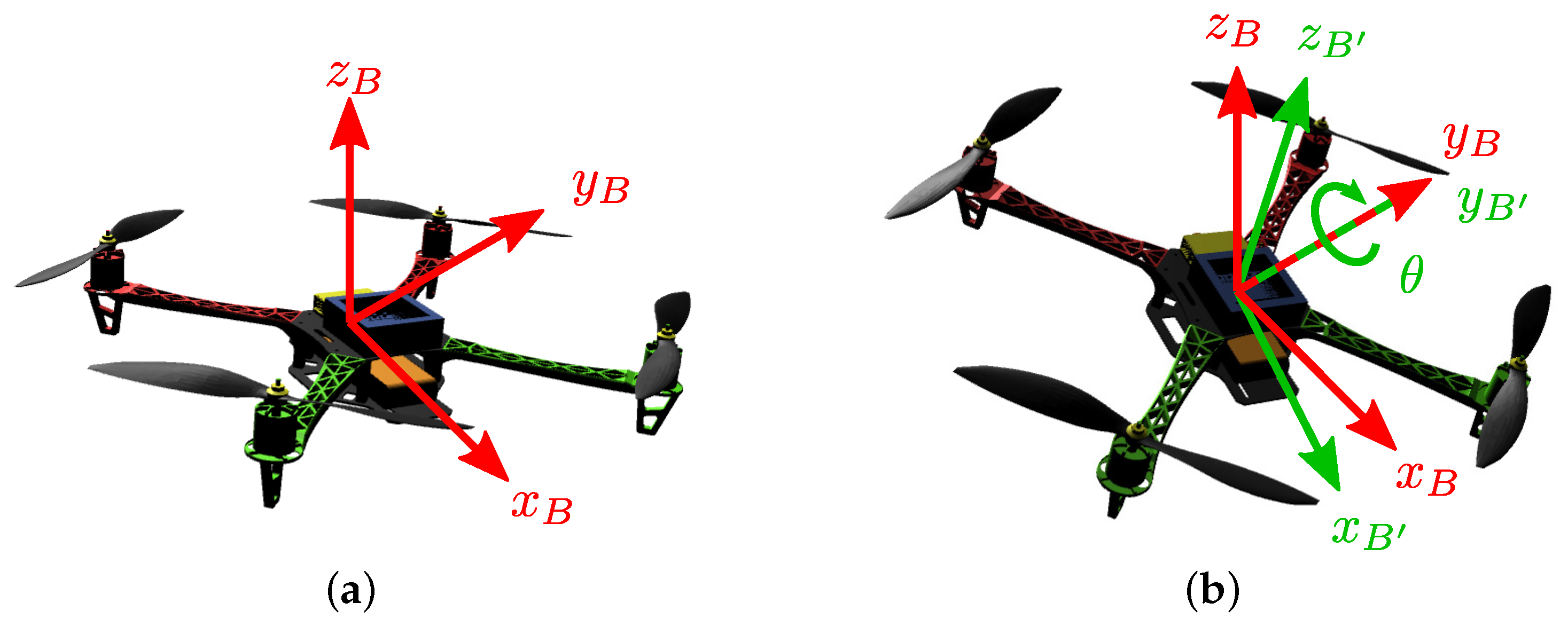
2.2.1. Quadrotor Kinematics

Kinematics studies the movement of bodies without considering the forces that generate it. In this way, quadrotor kinematics describes the quadrotor movements concerning the generalized coordinates.

As detailed before, the position of the quadrotor is given by its mass center location, i.e., $\mathit{\xi }={[x,y,z]}^T$, which is used to describe the translation movement. The rotation movement is related to the vector $\mathit{\eta }={[\varphi ,\theta ,\psi ]}^T$, and the convention of Euler angles $ZXY$. With the angles of the vector $\mathit{\eta }$, it can be established the orientation relationships between the frames $\{I\}$ and $\{B\}$ employing the elementary rotation matrices for each coordinate axis:

$$R_x(\varphi )=\left[\begin{array}{ccc}1& 0& 0\\ 0& cos\varphi & -sin\varphi \\ 0& sin\varphi & cos\varphi \end{array}\right]$$

(1)

$$R_y(\theta )=\left[\begin{array}{ccc}cos\theta & 0& sin\theta \\ 0& 1& 0\\ -sin\theta & 0& cos\theta \end{array}\right]$$

(2)

$$R_z(\psi )=\left[\begin{array}{ccc}cos\psi & -sin\psi & 0\\ sin\psi & cos\psi & 0\\ 0& 0& 1\end{array}\right]$$

(3)

Then, any vector $P^B$ in the coordinate system $\{B\}$ (e.g., the vector of a rotor position) can be written in the coordinate system $\{I\}$ using:

$$P^I=\mathit{\xi }+R_{zxy}{P}^B$$

(4)

where $R_{zxy}(\psi ,\varphi ,\theta )=R_z(\psi )R_x(\varphi )R_y(\theta )$.

2.2.2. Quadrotor Differential Kinematics

On the other hand, differential kinematics studies the motion relationships between the linear and angular velocities in a quadrotor concerning the translation and rotation ones. In this sense, the linear velocity in the quadrotor concerning the inertial system $\{I\}$ can be obtained as the time derivative of $\mathit{\xi }$ as:

$$\dot{\mathit{\xi }}={\left[\dot{x},\dot{y},\dot{z}\right]}^T$$

(5)

As for the angular velocity of the quadrotor, this requires additional analysis. Angular velocity is the rate of change in rotations around the three main axes in frame $\{I\}$ concerning time. This velocity is represented by the vector $\omega ={[p,q,r]}^T$, whose components are observed in Figure 3, where frame $\{I^{\prime }\}$ is the main frame $\{I\}$ translated to the mass center of the quadrotor. The vector $\omega$ is related to the rotation velocities $\dot{\mathit{\eta }}={[\dot{\varphi },\dot{\theta },\dot{\psi }]}^T$ by:

$$\mathit{\omega }=\dot{\theta }{\mathit{j}}_I+\dot{\varphi }{R}_y^T(\theta ){\mathit{i}}_I+\dot{\psi }{R}_y^T(\theta )R_x^T(\varphi ){\mathit{k}}_I$$

(6)

where ${\mathit{i}}_I$, ${\mathit{j}}_I$, and ${\mathit{k}}_I$, are the unit vectors of the main axes x, y, and z in $\{I\}$, respectively.

2.2.3. Quadrotor Dynamics

Dynamics studies the physical phenomena involved in the movement of the quadrotor. For this, the Lagrangian approach obtains the quadrotor dynamics. This approach requires the analysis of the energies in the system and involves the formulation of a mechanical Lagrangian $\mathcal{L}$. The Lagrangian is given by the difference between the total kinetic energy and the total potential energy of the quadrotor, as observed in (7).

$$\mathcal{L}=\mathcal{K}-\mathcal{U}$$

(7)

Potential energy is the ability of a body to carry out work depending on its configuration. In the case of the quadrotor, the potential energy depends on its vertical position and is given by:

$$\mathcal{U}=mgz$$

(8)

where m is the mass, and g is the acceleration of gravity.

On the other hand, kinetic energy is related to the motion of a body of a given mass. In this way, the kinetic energy of the quadrotor is due to two independent movements: the translation and the rotation. So, the total kinetic energy is the sum of the translational and rotational kinetic energies, respectively ${\mathcal{K}}_T$ and ${\mathcal{K}}_R$, as indicated in (9).

$$\mathcal{K}={\mathcal{K}}_T+{\mathcal{K}}_R$$

(9)

The translational kinetic energy of a mechanical system is given by [43]:

$${\mathcal{K}}_T=\frac{1}{2}m{\mathit{v}}^T\mathit{v}$$

(10)

where m is the body’s mass and $\mathit{v}$ is its linear velocity vector. In the quadrotor, the above linear velocity is $\mathit{v}=\dot{\mathit{\xi }}$.

Analogously, the rotational kinetic energy of a mechanical system is given by [43]:

$${\mathcal{K}}_R=\frac{1}{2}{\mathit{\omega }}^{T}I\mathit{\omega }$$

(11)

with $\omega$ as the angular velocity vector of the system and I as its moment of inertia. Since symmetric mass distribution is assumed in the quadrotor, the moment of inertia I of this system has the following form:

$$I=\left[\begin{array}{ccc}{I}_{xx}& 0& 0\\ 0& I_{yy}& 0\\ 0& 0& I_{zz}\end{array}\right]$$

(12)

where $I_{xx}$, $I_{yy}$, and $I_{zz}$ are the moments of inertia about the three coordinate axes.

Based on the Lagrangian $\mathcal{L}$ calculated before, the quadrotor can be modeled through the Lagrange equation of motion in (13) [44].

$$\frac{d}{dt}\left(\frac{\partial }{\partial \dot{\mathit{q}}}\mathcal{L}\left(\mathit{q},\dot{\mathit{q}}\right)\right)-\frac{\partial }{\partial \mathit{q}}\mathcal{L}\left(\mathit{q},\dot{\mathit{q}}\right)=0$$

(13)

where $\mathit{q}$ is the vector of generalized coordinates of the system, $\dot{\mathit{q}}$ is the vector with the first time derivative of these coordinates, and t is time.

Considering that the motion of the quadrotor is made up of rotation and translation independently, the equations of its motion can be obtained through two separate analyzes as denoted by (14).

$$\left\{\begin{array}{c}\frac{d}{dt}\left(\frac{\partial }{\partial \dot{\mathit{\xi }}}\mathcal{L}(\mathit{\xi },\dot{\mathit{\xi }})\right)-\frac{\partial }{\partial \mathit{\xi }}\mathcal{L}(\mathit{\xi },\dot{\mathit{\xi }})=0\hfill \\ \frac{d}{dt}\left(\frac{\partial }{\partial \dot{\mathit{\eta }}}\mathcal{L}(\mathit{\eta },\dot{\mathit{\eta }})\right)-\frac{\partial }{\partial \mathit{\eta }}\mathcal{L}(\mathit{\eta },\dot{\mathit{\eta }})=0\hfill \end{array}\right.$$

(14)

with $\mathcal{L}(\mathit{\xi },\dot{\mathit{\xi }})={\mathcal{K}}_T-\mathcal{U}$ and $\mathcal{L}(\mathit{\eta },\dot{\mathit{\eta }})={\mathcal{K}}_R$.

By calculating the derivatives in (14) and rearranging the terms obtained, the motion equation of the quadrotor can be expressed in the matrix closed-form as:

$$\left\{\begin{array}{c}{M}_T\left(\mathit{\xi }\right)\ddot{\mathit{\xi }}+{\mathit{g}}_T\left(\mathit{\xi }\right)=0\hfill \\ M_R\left(\mathit{\eta }\right)\ddot{\mathit{\eta }}+C_R\left(\mathit{\eta },\dot{\mathit{\eta }}\right)\dot{\mathit{\eta }}=0\hfill \end{array}\right.$$

(15)

where $M_T\left(\mathit{\xi }\right)$ and $M_R\left(\mathit{\eta }\right)$ are the inertia matrices for the translational and rotational equations, respectively, ${\mathit{g}}_T\left(\mathit{\xi }\right)$ is the translational gravity vector, and $C_R\left(\mathit{\eta },\dot{\mathit{\eta }}\right)$ is the rotational matrix of centrifugal and Coriolis forces. Full details of the motion equation terms (15) can be found in Appendix A.1.

2.2.4. Generalized Forces and Torques in the Quadrotor

The quadrotor is an under-actuated dynamic system. However, its four rotors can control its position and orientation as follows:

$$\left\{\begin{array}{c}{M}_T\left(\mathit{\xi }\right)\ddot{\mathit{\xi }}+{\mathit{g}}_T\left(\mathit{\xi }\right)=\mathit{f}\hfill \\ M_R\left(\mathit{\eta }\right)\ddot{\mathit{\eta }}+C_R\left(\mathit{\eta },\dot{\mathit{\eta }}\right)\dot{\mathit{\eta }}=\mathit{\tau }\hfill \end{array}\right.$$

(16)

where $\mathit{f}={[f_x,f_y,f_z]}^T$ and $\mathit{\tau }={[{\tau }_{\varphi },{\tau }_{\theta },{\tau }_{\psi }]}^T$ are respectively the vectors of forces and generalized torques that are produced by the rotational motion of the actuators.

In $\{B\}$, the thrust exerted by the four rotors is always vertical (collinear to axis $z_B$) and has the form:

$${\mathit{f}}_B={[0,0,f_{B,z}]}^T={[0,0,f_1+f_2+f_3+f_4]}^T$$

(17)

where $f_i$ is the thrust related to the torque ${\tau }_i$ of the i-th rotor. The thrust $f_i$ is obtained as in (18), with $l_h$ as the radial length of the propellers.

$$f_i=\frac{{\tau }_i}{l_h},i=1,2,3,4$$

(18)

In turn, the torque ${\tau }_i$ is related to the magnitude of the rotational speed ${\Omega }_i$ of the i-th rotor as shown in (19), where $k_r$ is a constant of proportionality of the same sign as ${\tau }_i$.

$${\tau }_i=k_r{\Omega }_i^2,i=1,2,3,4$$

(19)

Then, in $\{I\}$, the generalized force $\mathit{f}$, applied to translational dynamics, is given by:

$$\mathit{f}=R_{zxy}\left(\varphi ,\theta ,\psi \right){\mathit{f}}_B$$

(20)

On the other side, the components of the generalized torque $\mathit{\tau }$ are obtained by analyzing the possible quadrotor movements in Figure 4.

The movement of the rotors to hold the quadrotor in a fixed position in the air requires that all the rotors rotate at the same angular velocity to generate the upward thrust force as indicated in (21) and the direction described in Figure 4a. In the same figure, it can be seen that the direction of rotation of the consecutive rotors is inverse to prevent the quadrotor from making any rotation.

$${\Omega }_1={\Omega }_2={\Omega }_3={\Omega }_4$$

(21)

The roll motion (rotation around the $x_B$ axis) requires a difference in thrust produced by the rotors 3–4 concerning the rotors 1–2, as seen in Figure 4b. Then, the torque necessary to perform the roll motion is given by (22).

$${\tau }_{\varphi }={\tau }_3+{\tau }_4-{\tau }_1-{\tau }_2$$

(22)

Analogously, pitch motion (rotation around the $y_B$ axis) requires a difference in thrust produced by the rotors 1–4 concerning the rotors 2–3, as seen in Figure 4c. Therefore, the torque necessary to perform this motion is observed in (23).

$${\tau }_{\theta }={\tau }_4+{\tau }_1-{\tau }_2-{\tau }_3$$

(23)

Finally, the yaw movement (rotation around the vertical axis or $z_B$) is related to the torque ${\tau }_i$ perpendicular to the plane of rotation produced by all rotors, i.e., it requires a difference in thrust produced by the rotors 2–4 concerning the rotors 1–3 as seen in Figure 4d. Then the torque necessary to perform the yaw motion is given by (24).

$${\tau }_{\psi }={\tau }_1-{\tau }_2+{\tau }_3-{\tau }_4$$

(24)

The developed forms of the vectors $\mathit{f}$ and $\mathit{\tau }$ can be consulted in Appendix A.2.

2.2.5. Non-Conservative Effects in the Quadrotor

A more realistic model requires to include non-conservative effects such as friction. So, a model that considers frictions in the dynamics of rotation and translation can have the following form:

$$\left\{\begin{array}{c}{M}_T\left(\mathit{\xi }\right)\ddot{\mathit{\xi }}+{\mathit{g}}_T\left(\mathit{\xi }\right)+f_f(\dot{\mathit{\xi }})=\mathit{f}\hfill \\ M_R\left(\mathit{\eta }\right)\ddot{\mathit{\eta }}+C_R\left(\mathit{\eta },\dot{\mathit{\eta }}\right)\dot{\mathit{\eta }}+{\tau }_f(\dot{\mathit{\eta }})=\mathit{\tau }\hfill \end{array}\right.$$

(25)

where ${\mathit{f}}_f$ in (26) is the friction vector due to the translation velocity $\dot{\mathit{\xi }}$ of the quadrotor, and ${\mathit{\tau }}_f$ in (27) is the friction vector due to the rotation velocity $\dot{\mathit{\eta }}$ when the quadrotor interacts with the air.

$${\mathit{f}}_f={\left[f_{\dot{x}},f_{\dot{y}},f_{\dot{z}}\right]}^T$$

(26)

$${\mathit{\tau }}_f={[{\tau }_{\dot{\varphi }},{\tau }_{\dot{\theta }},{\tau }_{\dot{\psi }}]}^T$$

(27)

In this framework, a viscous friction is considered in the translational dynamics, so the components of ${\mathit{f}}_f$ in (26), are $f_{\dot{x}}=b_{\dot{x}}\dot{x}$, $f_{\dot{y}}=b_{\dot{y}}\dot{y}$ and $f_{\dot{z}}=b_{\dot{z}}\dot{z}$, with $b_{\dot{x}}$, $b_{\dot{y}}$ and $b_{\dot{z}}$ as viscous friction coefficients. Similarly, this type of friction is also considered for the dynamics of rotation and the components of ${\mathit{\tau }}_f$ in (27) are ${\tau }_{\dot{\varphi }}=b_{\dot{\varphi }}\dot{\varphi }$, ${\tau }_{\dot{\theta }}=b_{\dot{\theta }}\dot{\theta }$ and ${\tau }_{\dot{\psi }}=b_{\dot{\psi }}\dot{\psi }$, with $b_{\dot{\varphi }}$, $b_{\dot{\theta }}$ and $b_{\dot{\psi }}$ as viscous friction coefficients.

For completeness, the developed forms of ${\mathit{f}}_f$ and ${\mathit{\tau }}_f$ are presented in Appendix A.3.

2.3. Dynamic Simulation

The complete dynamic model of the quadrotor in (25), i.e., the equations of motion that describe the translation and rotation of this vehicle, can be utilized to perform a dynamic simulation. This simulation consists of determining the future states of a system from an initial configuration [45]. A state is the minimum set of variables that fully describe the behavior of a dynamical system at any instant of time [46]. For any mechanical system like the quadrotor, the state variables are typically the generalized coordinates and their first time derivatives. Then, the state vector $\mathit{\chi }$ for the quadrotor is composed of $\mathit{\xi }$ and $\mathit{\eta }$, and their first time derivatives $\dot{\mathit{\xi }}$ and $\dot{\mathit{\eta }}$ as follows:

$$\mathit{\chi }={[\mathit{\xi },\mathit{\eta },\dot{\mathit{\xi }},\dot{\mathit{\eta }}]}^T$$

(28)

Then, a state equation can be formulated based on $\mathit{\chi }$. The state equation is a differential equation that establishes a relationship between the current and future states of a system when it is subjected to a given input [47]:

$$\dot{\mathit{\chi }}=f(\mathit{\chi },\mathit{u},t)$$

(29)

with $\mathit{u}$ as the vector of the system inputs.

Using (25), the state equation of the quadrotor is in the form:

$$\dot{\mathit{\chi }}=\left[\begin{array}{c}\dot{\mathit{\xi }}\\ \dot{\mathit{\eta }}\\ \ddot{\mathit{\xi }}\\ \ddot{\mathit{\eta }}\end{array}\right]=\left[\begin{array}{c}\dot{\mathit{\xi }}\\ \dot{\mathit{\eta }}\\ M_T^{-1}\left(\mathit{\xi }\right)[\mathit{f}-{\mathit{g}}_T\left(\mathit{\xi }\right)-{\mathit{f}}_f(\dot{\mathit{\xi }})]\\ M_R^{-1}\left(\mathit{\eta }\right)[\mathit{\tau }-C_R\left(\mathit{\eta },\dot{\mathit{\eta }}\right)]\dot{\mathit{\eta }}-{\mathit{\tau }}_f(\dot{\mathit{\eta }})]\end{array}\right]$$

(30)

If an initial condition ${\mathit{\chi }}_0$ is imposed on the previous equation, it becomes an Initial Value Problem (IVP) like the one shown in (31). The IVP can be solved by some numerical integration method to simulate the quadrotor behavior. Although there is a vast diversity of sophisticated numerical integration methods, this framework adopts Euler’s method [48] (also known as ode1) due to its simplicity and low computational cost. Using Euler’s method, the future states of the quadrotor are calculated after a short time window $dt$ from a current time instant.

$$IVP=\left\{\begin{array}{c}\dot{\mathit{\chi }}=f(\mathit{\chi },\mathit{u},t)\hfill \\ \mathit{\chi }(0)={\mathit{\chi }}_0\hfill \end{array}\right.$$

(31)

Next, it is explained how this numerical simulation of the quadrotor integrates with the virtual environment.

2.4. Virtual Environment

Virtual Reality (VR) is a term used to refer to a type of human-computer interface that provides a realistic representation of the real world [49], typically through 3D geometries. One of the most widely used technologies today to create these interfaces is Unity 3D [50]. This tool is adopted to develop the proposed simulator. In this framework, the virtual environment is a 3D space that includes a virtual representation of the quadrotor, which can perform translation and rotation movements.

The adopted 3D quadrotor is a realistic model based on the device SM450, originally developed by Steven T and shared through the GrabCAD platform (https://grabcad.com/library/quadcopter-sm450-1 (accessed on 16 October 2021)). The above 3D model can be observed in Figure 5. Some of the elements in this 3D model can move freely to give a more realistic feel to the quadrotor. In this sense, the propellers’ rotation movement around the vertical axis is enabled. In addition, the above rotation can be animated during the simulation.

Regarding the rest of the virtual environment, various graphic elements represent objects or things found in the real world, such as trees, grass, terrains, and the sky. These elements have no actual interaction with the simulation, i.e., they are not considered in the dynamics of the quadrotor but can be included in the future through realistic collision handling. The utilized virtual elements are displayed in Figure 6.

2.5. Virtual Dynamic Simulation

At this point, it is possible to perform a dynamic simulation of the mathematical model of the quadrotor to obtain numerical information about its states. Likewise, there is a virtual representation of the quadrotor and its virtual operating environment in Unity 3D.

Then, the virtual simulation of the quadrotor consists of feeding the elements of the virtual environment with the information generated from the dynamic simulation. For this, it is essential to synchronize the update interval of the virtual environment in Unity 3D with the integration interval $dt$ used in Euler’s integration method not to affect the user’s perception of realism.

2.6. Virtual Teleoperation

Teleoperation can be defined as the continuous control of a remote slave robot by a human [51]. This definition fits naturally with the piloting of UAVs. In virtual teleoperation, the slave robot is virtual, and its remoteness is perceived through a virtual simulation, i.e., the human manipulates a virtual environment [51]. This kind of interaction is helpful in education, evaluation, and training [52].

The teleoperation algorithm proposed in this framework takes as inputs the commands triggered by the human user. They indicate how the quadrotor should move in terms of its generalized torques and forces. It is necessary to define which operations the user can perform through a master device. Even when there are very specialized master devices, gamepads are used more and more frequently to control UAVs. The above is because these game devices meet several usability criteria such as reduced size, portability, adaptability, universality, and ergonomics and can be acquired at affordable costs [53]. So, the Xbox Series gamepad is adopted as the master device, and its enabled commands are depicted in Figure 7. The commands established for this device develop the elevation, yaw, pitch, and roll movements in the quadrotor. It is important to highlight that although a gamepad is adopted to develop this framework, it is possible to carry out a mapping similar to the one carried out below between the input mechanisms of a more specialized device and the actions in the UAV.

The teleoperation algorithm in Algorithm 1 is proposed in this framework based on the above interactions. At every instant $dt$ in the virtual dynamic simulation, this algorithm handles the commands of the master device as follows:

• Elevation (lines 1–5 in Algorithm 1): Allows takeoff, landing, and keeping the quadrotor in the air. For this, the reference height $z_d$ varies proportionally to the positional value of the left stick for the vertical axis $u_{LSV}\in [-1,1]$ using the constant $k_z$. This reference value is set to $z_d=0$ when $z_d<0$ to avoid trespassing the floor. Then, $z_d$ is utilized to calculate the vertical thrust $f_{B,z}$ by a Proportional Integral Derivative (PID) controller with the gravity compensation term $mg$, where $k_{p,z}$, $k_{i,z}$, and $k_{d,z}$ are the proportional, integral, and derivative gains, respectively.
• Yaw (lines 6–8 in Algorithm 1): Changes the direction the front of the quadrotor is pointing, to the left or to the right (it is assumed that the front of the quadrotor coincides with the positive direction of the axis $x_B$). In this case, the desired yaw angle ${\psi }_d$ takes a value proportional to the positional value of the left stick for the horizontal axis $u_{LSH}\in [-1,1]$ with the constant $k_{\psi }$. A PID controller is also adopted to develop the torque ${\tau }_{\psi }$ with $k_{p,\psi }$, $k_{i,\psi }$, and $k_{d,\psi }$ as the proportional, integral, and derivative gains, respectively.
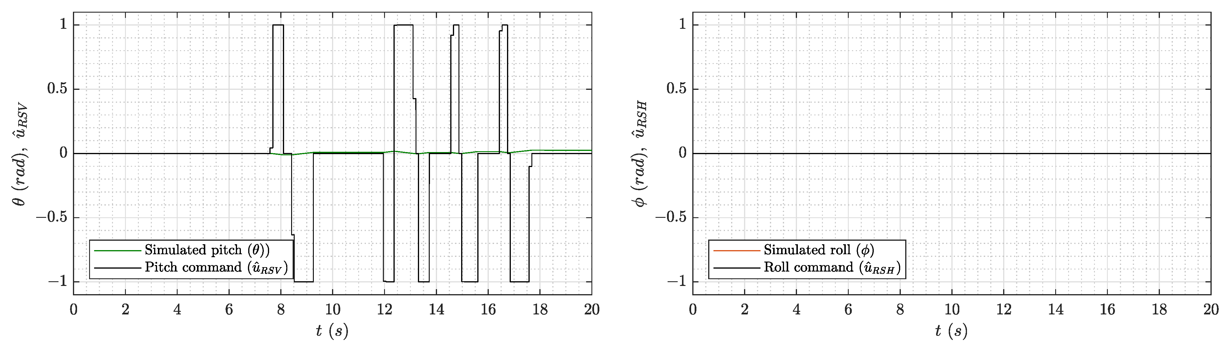
• Pitch (lines 9–16 in Algorithm 1): Produces a forward and backward movement of the quadrotor in the direction the front of the quadrotor is pointing. Here, the desired pitch angle $\theta$ is proportionally modified by the positional value of the right stick for the vertical axis $u_{RSV}\in [-1,1]$ based on the constant $k_{\theta }$. Additionally, the reference is set as ${\theta }_d=0$ to stop the vehicle when $u_{RSV}=0$. Moreover, the value of ${\theta }_d$ is bounded in the interval $[-\pi /4,\pi /4]$ to avoid singularities. As in the above case, a PID controller is included to develop the torque ${\tau }_{\theta }$, where $k_{p,\theta }$, $k_{i,\theta }$, and $k_{d,\theta }$ are the proportional, integral, and derivative parameters, respectively.
• Roll (lines 17–24 in Algorithm 1): Generates movement towards the sides of the quadrotor, i.e., in the direction of the axis $y_B$. In this case, the desired roll angle ${\varphi }_d$ is proportionally modified by the positional value of the right stick for the horizontal axis $u_{RSH}\in [-1,1]$ using the constant $k_{\varphi }$. This reference is set as ${\varphi }_d=0$ to stop the vehicle when $u_{RSH}=0$. As in the pitch movement, the value of ${\varphi }_d$ is bounded in the interval $[-\pi /4,\pi /4]$ to avoid singularities. Analogously, a PID controller is included to develop the torque ${\tau }_{\varphi }$, where $k_{p,\varphi }$, $k_{i,\varphi }$, and $k_{d,\varphi }$ are the proportional, integral, and derivative parameters, respectively.

From the above teleoperation algorithm, the input scaling constants $k_z$, $k_{\psi }$, $k_{\theta }$, and $k_{\varphi }$; the proportional gains $k_{p,z}$, $k_{p,\psi }$, $k_{p,\theta }$, and $k_{p,\varphi }$; the integral gains $k_{i,z}$, $k_{i,\psi }$, $k_{i,\theta }$, and $k_{i,\varphi }$; and the derivative gains $k_{d,z}$, $k_{d,\psi }$, $k_{d,\theta }$, and $k_{d,\varphi }$ must be adjusted correctly to match the behavior of a real-world teleoperated quadrotor.

Algorithm 1: Teleoperation algorithm

2.7. Simulator Optimization

The virtual teleoperated simulator developed so far includes elements that provide a feeling of realism to a certain extent. However, as mentioned before, this feature also depends on the suitable adjustment of the parameters in the teleoperation algorithm. Nevertheless, tuning these parameters is not a trivial task due to the highly non-linear relationships between the inputs and the considered movements in the quadrotor.

For the above fact, the meta-heuristic optimization approach is used in this framework to tune the teleoperation parameters [54]. In this approach, a mathematical programming problem is stated first. Then, the problem is solved by a meta-heuristic optimizer, and the solution includes a suitable set of parameters.

Because the simulation needs to be as close to reality as possible, the flight information of a real-world quadrotor and its interactions with the human operator is required. This information guides the search for the best teleoperation parameters. It can be acquired from the sensors included in any real-world vehicle, such as the Inertial Measurement Unit (IMU), the gyroscope, and the magnetometer, among other alternatives.

In this framework, it is assumed that the height $\widehat{z}$, the yaw angle $\widehat{\psi }$, the pitch angle $\widehat{\theta }$, and the roll angle $\widehat{\varphi }$ values, as well as the input control actions for the elevation ${\widehat{u}}_{LSV}$, the yaw movement ${\widehat{u}}_{LSH}$, the pitch movement ${\widehat{u}}_{RSV}$, and the roll movement ${\widehat{u}}_{RSH}$ can be acquired from the real-world quadrotor.

Therefore, the mathematical programming problem for the optimization of the teleoperation parameters can be stated as:

$${\mathbf{min}}_{\mathit{p}\in \Omega }J(\mathit{p})=J_z(\mathit{p})+J_{\psi }(\mathit{p})+J_{\theta }(\mathit{p})+J_{\varphi }(\mathit{p})$$

(32)

where the vector $\mathit{p}$ includes the parameters of the teleoperation algorithm, $\Omega$ is the search space given by the lower and upper bounds of each parameter, and $J_z(\mathit{p})$, $J_{\psi }(\mathit{p})$,$J_{\theta }(\mathit{p})$, and $J_{\varphi }(\mathit{p})$ are the objective functions related to the Integral Square Error (ISE) index [55] calculated over the errors $e_z(t)=\widehat{z}(t)-z(t)$, $e_{\psi }(t)=\widehat{\psi }(t)-\psi (t)$, $e_{\theta }(t)=\widehat{\theta }(t)-\theta (t)$, and $e_{\varphi }(t)=\widehat{\varphi }(t)-\varphi (t)$ for $t\in [0,t_f]$ as follows:

$$J_z(\mathit{p})=ISE(e_z(t))={\int }_{t=0}^{t_f}(\widehat{z}(t)-z(t))dt$$

(33)

$$J_{\psi }(\mathit{p})=ISE(e_{\psi }(t))={\int }_{t=0}^{t_f}(\widehat{\psi }(t)-\psi (t))dt$$

(34)

$$J_{\theta }(\mathit{p})=ISE(e_{\theta }(t))={\int }_{t=0}^{t_f}(\widehat{\theta }(t)-\theta (t))dt$$

(35)

$$J_{\varphi }(\mathit{p})=ISE(e_{\varphi }(t))={\int }_{t=0}^{t_f}(\widehat{\varphi }(t)-\varphi (t))dt$$

(36)

In the above functions, $z(t)$, $\psi (t)$, $\theta (t)$, and $\varphi (t)$ are obtained from the dynamic simulation of the quadrotor considering ${\widehat{u}}_{LSV}$, ${\widehat{u}}_{LSH}$, ${\widehat{u}}_{RSV}$, and ${\widehat{u}}_{RSH}$ as the inputs.

Therefore the problem in (32) aims to find the parameters of the teleoperation algorithm that minimize the differences between the behavior of the simulated and the real-world quadrotors when both receive the same inputs. Meta-heuristic optimizers from swarm intelligence and evolutionary computation can solve this problem [56].

3. Results and Discussion

The effectiveness of the proposed framework in developing a realistic simulator for the quadrotor is evaluated in this section. For this, the behavior of the simulated quadrotor is compared to that of a real-world quadrotor.

The device utilized to perform the comparisons is the DJI Ryze Tello quadrotor controlled by the GameSir T1d gamepad, as observed in Figure 8. The dynamic parameters of the quadrotor model are proposed based on the characteristics of this device and an arbitrary set of environmental conditions. These parameters are displayed in

Table 1. Dynamic parameters of the quadrotor.

Parameter	Nominal Value
m	0.225 (kg)
g	9.81 (m/s2)
$I_{xx}$	5.0 × 10−3 (kg m2)
$I_{yy}$	5.0 × 10−3 (kg m2)
$I_{zz}$	5.0 × 10−3 (kg m2)
$l_h$	0.042 (m)
$b_{\dot{x}}$	1.0 (N s/m)
$b_{\dot{y}}$	1.0 (N s/m)
$b_{\dot{z}}$	1.0 (N s/m)
$b_{\dot{\varphi }}$	0.5 (N m s/rad)
$b_{\dot{\theta }}$	0.5 (N m s/rad)
$b_{\dot{\psi }}$	0.5 (N m s/rad)

. On the other hand, interval $dt=1(\mathrm{ms})$ is used to perform the dynamic simulation and as the update rate of the virtual environment.

Concerning the teleoperation algorithm, its parameters are tuned with the rand/1/bin variant of Differential Evolution (DE) [57]. This well-known meta-heuristic optimizer has been successfully utilized in applications from various contexts [58]. The hyper-parameters selected for this optimizer are a maximum number of generations $G_{max}=1000$, a population size $NP=20$, and typical choices of the crossover rate $CR=0.5$ and the scaling factor $F=0.5$ [59]. Moreover, every searched parameter’s lower and upper bounds are set as $lb=0$ and $ub=30$, respectively. For the optimization of these parameters, a test flight is performed with the DJI Ryze Tello quadrotor during $t_f$ = 20 (s) to gather the required data for the problem in (32), i.e., the values of $\widehat{z}$, $\widehat{psi}$, $\widehat{\theta }$, and $\widehat{\varphi }$ and the input commands of the controller ${\widehat{u}}_{LSV}$, ${\widehat{u}}_{LSH}$, ${\widehat{u}}_{RSV}$, and ${\widehat{u}}_{RSH}$. Like any other commercial vehicle, this quadrotor is equipped with sensors that allow monitoring and control. The information is stored as a standard flight log file, and the required data is extracted using the DatCon tool (https://datfile.net/DatCon/intro.html (accessed on 16 October 2021)). It is important to mention that, due to the different sampling frequencies of the sensors, it is unlikely that the required information can be sampled every $dt$. So, a standardization procedure is needed to work with the available data. This standardization consists of filling the unavailable values at a given instant with the available values of the previous instant. In this way, the standardized information acquired from the test flight is displayed in Figure 9. Finally, DE performs the optimization using the above information, and the resulting teleoperation parameters are observed in

Table 2. Optimized teleoperation parameters.

Type	Parameter	Value
Input	$k_z$	0.0028
scaling	$k_{\psi }$	0.0027
constants	$k_{\theta }$	0.9879
	$k_{\varphi }$	0.3030
Proportional	$k_{p,z}$	12.3973
gains	$k_{p,\psi }$	26.9075
	$k_{p,\theta }$	0.3159
	$k_{p,\varphi }$	0.1176
Integral	$k_{i,z}$	0.0146
gains	$k_{i,\psi }$	0.0001
	$k_{i,\theta }$	0.0363
	$k_{i,\varphi }$	0.0116
Derivative	$k_{d,z}$	16.4687
gains	$k_{d,\psi }$	0.0022
	$k_{d,\theta }$	0.0029
	$k_{d,\varphi }$	0.0781

.

Table 3. Objective function values.

Objective Function	Value
$J_z(\mathit{p})$	0.8204
$J_{\psi }(\mathit{p})$	0.2148
$J_{\theta }(\mathit{p})$	0.0537
$J_{\varphi }(\mathit{p})$	0.0013
$J(\mathit{p})$	1.0903

shows the objective function values obtained with the optimized teleoperation parameters in Table 2. In the first table, the small values of the objective functions denote a response of the simulated quadrotor close to the behavior of the real quadrotor when both receive the same input commands. This response can be observed in Figure 10. If the results in Figure 9 and Figure 10 are compared, a similar shape is observed for the simulated and real data, but the response of the simulated quadrotor is smoother.

The obtained results for the quadrotor study case indicate that the proposed framework can be used to develop realistic virtual simulators for the teleoperation of UAVs.

The optimized configuration above is used in the final simulator shown in Figure 11. Finally, an arbitrary flight is carried out in the simulator (i.e., using arbitrary commands from the Xbox Series gamepad) to verify its operation. The obtained log is observed in Figure 12. A suitable and smooth response to the user commands is observed in that figure.

4. Conclusions and Future Work

Based on the necessity of simulation tools for UAVs remotely controlled by human operators, this work proposes a framework to build realistic virtual simulators for the teleoperation of these vehicles. The quadrotor is adopted as the study case.

The framework elements consider the modeling, the dynamic simulation, the interconnection of the dynamic simulation with a virtual environment, and the interaction with the user through a teleoperation scheme.

In each of the previous elements, realism is incorporated into the simulator. The modeling fully describes the behavior of a UAV and considers the non-conservative phenomena of the operating environment to develop a dynamic simulation close to reality. The virtual environment includes a realistic representation of the UAV and other components familiar to a human operator. Finally, the teleoperation scheme is optimized with a meta-heuristic optimizer to match the behavior of a real-world teleoperated UAV.

The response of the simulated UAV is compared with that of a real-world one, and similar behaviors are obtained. The above describes the effectiveness of the proposed framework.

In addition, some advantages of simulators that can be developed through this framework include obtaining an explicit realistic model of the UAV, which can be used in tasks such as identification and controller design. Also, the model can be supplemented with more specific models of the vehicle elements, e.g., the actuators, to obtain simulations closer to reality. Even when the case study of this framework is developed in Unity 3D, it does not depend on a specific technology or platform. In this way, a simulator based on this framework can be implemented using available technology and accessed from different platforms, increasing the availability of this proposal.

In future work, the realism in the simulator can be improved by considering a more detailed model of the UAV. In this sense, the dynamics of rotors and drivers can be coupled to the model obtained in this work. Also, an enhanced proposal could include the interactions of the UAV with other objects in the virtual environment, e.g., through realistic collision handling. Moreover, simulating the operation of some sensors can improve the feedback to the human user. Finally, the feedback response can be enhanced by using haptic responses.

References

1. Abushahma, R.I.H.; Ali, M.A.M.; Rahman, N.A.A.; Al-Sanjary, O.I. Comparative Features of Unmanned Aerial Vehicle (UAV) for Border Protection of Libya: A Review. In Proceedings of the 2019 IEEE 15th International Colloquium on Signal Processing Its Applications (CSPA), Penang, Malaysia, 8–9 March 2019; pp. 114–119. [Google Scholar] [CrossRef]
2. Maimaitijiang, M.; Sagan, V.; Sidike, P.; Daloye, A.M.; Erkbol, H.; Fritschi, F.B. Crop Monitoring Using Satellite/UAV Data Fusion and Machine Learning. Remote Sens. 2020, 12, 1357. [Google Scholar] [CrossRef]
3. Huang, J.; Tian, G.; Zhang, J.; Chen, Y. On Unmanned Aerial Vehicles Light Show Systems: Algorithms, Software and Hardware. Appl. Sci. 2021, 11, 7687. [Google Scholar] [CrossRef]
4. Subchan, S.; White, B.; Tsourdos, A.; Shanmugavel, M.; Żbikowski, R. Dubins Path Planning of Multiple UAVs for Tracking Contaminant Cloud. 17th IFAC World Congress. IFAC Proc. Vol. 2008, 41, 5718–5723. [Google Scholar] [CrossRef] [Green Version]
5. Fong, T.; Thorpe, C. Vehicle Teleoperation Interfaces. Auton. Robot. 2001, 11, 9–18. [Google Scholar] [CrossRef]
6. Mansfield, K.; Eveleigh, T.; Holzer, T.H.; Sarkani, S. Unmanned aerial vehicle smart device ground control station cyber security threat model. In Proceedings of the 2013 IEEE International Conference on Technologies for Homeland Security (HST), Waltham, MA, USA, 12–14 November 2013; pp. 722–728. [Google Scholar] [CrossRef]
7. Liu, X.; Zhou, H. Unmanned Water-Powered Aerial Vehicles: Theory and Experiments. IEEE Access 2019, 7, 15349–15356. [Google Scholar] [CrossRef]
8. Liaw, J.F.; Tsai, P.H. Target prediction to improve human errors in robot teleoperation system. In Proceedings of the 2017 International Conference on Applied System Innovation (ICASI), Sapporo, Japan, 13–17 May 2017; pp. 1094–1097. [Google Scholar] [CrossRef]
9. Isop, W.A.; Gebhardt, C.; Nägeli, T.; Fraundorfer, F.; Hilliges, O.; Schmalstieg, D. High-Level Teleoperation System for Aerial Exploration of Indoor Environments. Front. Robot. AI 2019, 6, 95. [Google Scholar] [CrossRef] [Green Version]
10. Besada, J.A.; Campaña, I.; Bergesio, L.; Bernardos, A.M.; de Miguel, G. Drone Flight Planning for Safe Urban Operations: UTM Requirements and Tools. In Proceedings of the 2019 IEEE International Conference on Pervasive Computing and Communications Workshops (PerCom Workshops), Kyoto, Japan, 11–15 March 2019; pp. 924–930. [Google Scholar] [CrossRef]
11. Mademlis, I.; Mygdalis, V.; Nikolaidis, N.; Montagnuolo, M.; Negro, F.; Messina, A.; Pitas, I. High-Level Multiple-UAV Cinematography Tools for Covering Outdoor Events. IEEE Trans. Broadcast. 2019, 65, 627–635. [Google Scholar] [CrossRef]
12. Millet, P.; Grinberg, M.; Jahre, M. Challenges in the Realm of Embedded Real-Time Image Processing. In Towards Ubiquitous Low-Power Image Processing Platforms; Jahre, M., Göhringer, D., Millet, P., Eds.; Springer International Publishing: Cham, Switzerland, 2021; pp. 3–13. [Google Scholar] [CrossRef]
13. Ashokkumar, C.R.; York, G.W.P. Data science for decision aiding UAV control. In Proceedings of the 2017 International Conference on Unmanned Aircraft Systems (ICUAS), Miami, FL, USA, 13–16 June 2017; pp. 11–15. [Google Scholar] [CrossRef]
14. Zhang, R.; Cao, S.; Zhao, K.; Yu, H.; Hu, Y. A Hybrid-Driven Optimization Framework for Fixed-Wing UAV Maneuvering Flight Planning. Electronics 2021, 10, 2330. [Google Scholar] [CrossRef]
15. Ribeiro, R.; Ramos, J.; Safadinho, D.; Reis, A.; Rabadão, C.; Barroso, J.; Pereira, A. Web AR Solution for UAV Pilot Training and Usability Testing. Sensors 2021, 21, 1456. [Google Scholar] [CrossRef]
16. Stöcker, C.; Bennett, R.; Nex, F.; Gerke, M.; Zevenbergen, J. Review of the Current State of UAV Regulations. Remote Sens. 2017, 9, 459. [Google Scholar] [CrossRef] [Green Version]
17. Fuller, E. The Educational Road is Open. Bull. Natl. Assoc. Second. Sch. Princ. 1944, 28, 7–11. [Google Scholar] [CrossRef]
18. Ballesteros, R.; Ortega, J.F.; Hernández, D.; Moreno, M.A. Applications of georeferenced high-resolution images obtained with unmanned aerial vehicles. Part I: Description of image acquisition and processing. Precis. Agric. 2014, 15, 579–592. [Google Scholar] [CrossRef]
19. Hing, J.T.; Sevcik, K.W.; Oh, P.Y. Improving unmanned aerial vehicle pilot training and operation for flying in cluttered environments. In Proceedings of the 2009 IEEE/RSJ International Conference on Intelligent Robots and Systems, St. Louis, MO, USA, 10–15 October 2009; pp. 5641–5646. [Google Scholar] [CrossRef]
20. Turk, I.; Ozbek, E.; Ekici, S.; Karakoc, T.H. A conceptual design of a solar powered UAV and assessment for continental climate flight conditions. Int. J. Green Energy 2021, 1–11. [Google Scholar] [CrossRef]
21. Kinoshita, T.; Imado, F. The Application of an UAV Flight Simulator - The Development of a New Point Mass Model for an Aircraft. In Proceedings of the 2006 SICE-ICASE International Joint Conference, Busan, Korea, 18–21 October 2006; pp. 4378–4383. [Google Scholar] [CrossRef]
22. Orbea, D.; Moposita, J.; Aguilar, W.G.; Paredes, M.; León, G.; Jara-Olmedo, A. Math Model of UAV Multi Rotor Prototype with Fixed Wing Aerodynamic Structure for a Flight Simulator. In Augmented Reality, Virtual Reality, and Computer Graphics; De Paolis, L.T., Bourdot, P., Mongelli, A., Eds.; Springer International Publishing: Cham, Switzerland, 2017; pp. 199–211. [Google Scholar]
23. Fernando, H.C.T.E.; De Silva, A.T.A.; De Zoysa, M.D.C.; Dilshan, K.A.D.C.; Munasinghe, S.R. Modelling, simulation and implementation of a quadrotor UAV. In Proceedings of the 2013 IEEE 8th International Conference on Industrial and Information Systems, Peradeniya, Sri Lanka, 17–20 December 2013; pp. 207–212. [Google Scholar] [CrossRef]
24. Jin, G.D.; Gu, L.X.; Lu, L.B. UAV Simulator-Based Simulation of Flight Control System. In Proceedings of the 2009 International Workshop on Intelligent Systems and Applications, Hangzhou, China, 26–27 August 2009; pp. 1–4. [Google Scholar] [CrossRef]
25. Siddiqui, K.T.A.; Feil-Seifer, D.; Jiang, T.; Jose, S.; Liu, S.; Louis, S. Development of a Swarm UAV Simulator Integrating Realistic Motion Control Models For Disaster Operations. In Proceedings of the ASME 2017 Dynamic Systems and Control Conference, Tysons, VA, USA, 11–13 October 2017; pp. 1–10. [Google Scholar] [CrossRef] [Green Version]
26. Rzucidło, P. Unmanned air vehicle research simulator-prototyping and testing of control and navigation systems. Solid State Phenom. 2013, 198, 266–271. [Google Scholar] [CrossRef]
27. Manaï, M.; Desbiens, A.; Gagnon, E. Identification of a UAV and Design of a Hardware-in-the-Loop System for Nonlinear Control Purposes. In Proceedings of the AIAA Guidance, Navigation, and Control Conference and Exhibit, Minneapolis, MN, USA, 13–16 August 2012. [Google Scholar] [CrossRef]
28. Lizarraga, M.; Dobrokhodov, V.; Elkaim, G.; Curry, R.; Kaminer, I. Simulink Based Hardware-in-the-Loop Simulator for Rapid Prototyping of UAV Control Algorithms. In Proceedings of the AIAA Infotech@Aerospace Conference, Seattle, WA, USA, 6–9 April 2009. [Google Scholar] [CrossRef] [Green Version]
29. Ates, S.; Bayezit, I.; Inalhan, G. Design and Hardware-in-the-Loop Integration of a UAV Microavionics System in a Manned–Unmanned Joint Airspace Flight Network Simulator. J. Intell. Robot. Syst. 2009, 54, 359–386. [Google Scholar] [CrossRef]
30. Lugo-Cárdenas, I.; Salazar, S.; Lozano, R. The MAV3DSim hardware in the loop simulation platform for research and validation of UAV controllers. In Proceedings of the 2016 International Conference on Unmanned Aircraft Systems (ICUAS), Arlington, VA, USA, 7–10 June 2016; pp. 1335–1341. [Google Scholar] [CrossRef]
31. Meng, W.; Hu, Y.; Lin, J.; Lin, F.; Teo, R. ROS+unity: An efficient high-fidelity 3D multi-UAV navigation and control simulator in GPS-denied environments. In Proceedings of the IECON 2015—41st Annual Conference of the IEEE Industrial Electronics Society, Yokohama, Japan, 9–12 November 2015; pp. 2562–2567. [Google Scholar] [CrossRef]
32. Zhang, M.; Qin, H.; Lan, M.; Lin, J.; Wang, S.; Liu, K.; Lin, F.; Chen, B.M. A high fidelity simulator for a quadrotor UAV using ROS and Gazebo. In Proceedings of the IECON 2015—41st Annual Conference of the IEEE Industrial Electronics Society, Yokohama, Japan, 9–12 November 2015; pp. 2846–2851. [Google Scholar] [CrossRef]
33. Baidya, S.; Shaikh, Z.; Levorato, M. FlyNetSim: An Open Source Synchronized UAV Network Simulator Based on Ns-3 and Ardupilot. In Proceedings of the 21st ACM International Conference on Modeling, Analysis and Simulation of Wireless and Mobile Systems, MSWIM ’18, Montreal, QC, Canada, 28 October–2 November 2018; Association for Computing Machinery: New York, NY, USA, 2018; pp. 37–45. [Google Scholar] [CrossRef]
34. Ferlini, A.; Wang, W.; Pau, G. Corner-3D: A RF Simulator for UAV Mobility in Smart Cities. In Proceedings of the ACM SIGCOMM 2019 Workshop on Mobile AirGround Edge Computing, Systems, Networks, and Applications, MAGESys’19, Beijing, China, 19 August 2019; Association for Computing Machinery: New York, NY, USA, 2019; pp. 22–28. [Google Scholar] [CrossRef]
35. Mcmanus, I.; Greer, D.; Walker, R. Uav avionics’ hardware in the loop’simulator. In Proceedings of the 10th Australian International Aerospace Congress, Barton, Australia, 29 July–1 August 2003; pp. 1–7. [Google Scholar]
36. Garcia, R.; Barnes, L. Multi-UAV Simulator Utilizing X-Plane. In Proceedings of the 2nd International Symposium on UAVs, Reno, NV, USA, 8–10 June 2009; Valavanis, K.P., Beard, R., Oh, P., Ollero, A., Piegl, L.A., Shim, H., Eds.; Springer: Dordrecht, The Netherlands, 2010; pp. 393–406. [Google Scholar] [CrossRef]
37. De Rango, F.; Palmieri, N.; Santamaria, A.F.; Potrino, G. A simulator for UAVs management in agriculture domain. In Proceedings of the 2017 International Symposium on Performance Evaluation of Computer and Telecommunication Systems (SPECTS), Seattle, WA, USA, 9–12 July 2017; pp. 1–8. [Google Scholar] [CrossRef]
38. Mueller, M.; Smith, N.; Ghanem, B. A Benchmark and Simulator for UAV Tracking. In Proceedings of the Computer Vision—ECCV 2016, Amsterdam, The Netherlands, 11–14 October 2016; Leibe, B., Matas, J., Sebe, N., Welling, M., Eds.; Springer International Publishing: Cham, Switzerland, 2016; pp. 445–461. [Google Scholar]
39. Imado, F.; Abe, S.; Kinoshita, T. The Development of Three-Dimensional Scale Model UAV Simulator. In Proceedings of the 2006 SICE-ICASE International Joint Conference, Busan, Korea, 18–21 October 2006; pp. 4921–4925. [Google Scholar] [CrossRef]
40. Al-Mousa, A.; Sababha, B.H.; Al-Madi, N.; Barghouthi, A.; Younisse, R. UTSim: A framework and simulator for UAV air traffic integration, control, and communication. Int. J. Adv. Robot. Syst. 2019, 16, 1729881419870937. [Google Scholar] [CrossRef] [Green Version]
41. Shah, S.; Dey, D.; Lovett, C.; Kapoor, A. AirSim: High-Fidelity Visual and Physical Simulation for Autonomous Vehicles. In Proceedings of the Field and Service Robotics, Zurich, Switzerland, 12–15 September 2017. [Google Scholar]
42. Zhang, F.; Lyu, X.; Wang, Y.; Gu, H.; Li, Z. Modeling and Flight Control Simulation of a Quadrotor Tailsitter VTOL UAV. In Proceedings of the AIAA Modeling and Simulation Technologies Conference, Grapevine, TX, USA, 9–13 January 2017. [Google Scholar] [CrossRef]
43. Spong, M.W.; Hutchinson, S.; Vidyasagar, M. Robot Modeling and Control; John Wiley & Sons: Hoboken, NJ, USA, 2020. [Google Scholar]
44. Wells, D.A. Schaum’s Outline of Lagrangian Dynamics; Schaum’s Outlines; McGraw-Hill: New York, NY, USA, 1967. [Google Scholar]
45. Wit, C.D.; Rabbinge, R. Systems Analysis and Dynamic Simulation 1. EPPO Bull. 1979, 9, 149–153. [Google Scholar] [CrossRef] [Green Version]
46. Wang, Q.; Wang, L.; Qin, W.; Shen, Q. A local observability analysis method for a time-varying nonlinear system and its application in the continuous self-calibration system. Sci. China Inf. Sci. 2020, 64, 11920. [Google Scholar] [CrossRef]
47. Lafortune, S.; Sengupta, R.; Kaufman, D.E.; Smith, R.L. Dynamic system-optimal traffic assignment using a state space model. Transp. Res. Part B Methodol. 1993, 27, 451–472. [Google Scholar] [CrossRef] [Green Version]
48. Fathoni, M.F.; Wuryandari, A.I. Comparison between Euler, Heun, Runge-Kutta and Adams-Bashforth-Moulton integration methods in the particle dynamic simulation. In Proceedings of the 2015 4th International Conference on Interactive Digital Media (ICIDM), Bandung, Indonesia, 1–5 December 2015; pp. 1–7. [Google Scholar] [CrossRef]
49. Zheng, J.; Chan, K.; Gibson, I. Virtual reality. IEEE Potentials 1998, 17, 20–23. [Google Scholar] [CrossRef]
50. Okita, A. Learning C# Programming with Unity 3D; AK Peters/CRC Press: Natick, MA, USA, 2019. [Google Scholar]
51. Su, H.; Qi, W.; Yang, C.; Sandoval, J.; Ferrigno, G.; De Momi, E. Deep neural network approach in robot tool dynamics identification for bilateral teleoperation. IEEE Robot. Autom. Lett. 2020, 5, 2943–2949. [Google Scholar] [CrossRef]
52. Bolopion, A.; Régnier, S. A review of haptic feedback teleoperation systems for micromanipulation and microassembly. IEEE Trans. Autom. Sci. Eng. 2013, 10, 496–502. [Google Scholar] [CrossRef] [Green Version]
53. Rupp, M.A.; Oppold, P.; McConnell, D.S. Evaluating input device usability as a function of task difficulty in a tracking task. Ergonomics 2015, 58, 722–735. [Google Scholar] [CrossRef]
54. Rodríguez-Molina, A.; Mezura-Montes, E.; Villarreal-Cervantes, M.G.; Aldape-Pérez, M. Multi-objective meta-heuristic optimization in intelligent control: A survey on the controller tuning problem. Appl. Soft Comput. 2020, 93, 106342. [Google Scholar] [CrossRef]
55. Yeşil, E.; Güzelkaya, M.; Eksin, İ. Self tuning fuzzy PID type load and frequency controller. Energy Convers. Manag. 2004, 45, 377–390. [Google Scholar] [CrossRef]
56. Caraffini, F.; Santucci, V.; Milani, A. Evolutionary Computation & Swarm Intelligence; MDPI: Basel, Switzerland, 2020. [Google Scholar]
57. Kenneth, V. Price. An introduction to differential evolution. In New Ideas in Optimization; McGraw-Hill: London, UK, 1999; pp. 79–108. [Google Scholar]
58. Pant, M.; Zaheer, H.; Garcia-Hernandez, L.; Abraham, A. Differential Evolution: A review of more than two decades of research. Eng. Appl. Artif. Intell. 2020, 90, 103479. [Google Scholar] [CrossRef]
59. Mezura-Montes, E.; Velázquez-Reyes, J.; Coello Coello, C.A. A Comparative Study of Differential Evolution Variants for Global Optimization. In Proceedings of the 8th Annual Conference on Genetic and Evolutionary Computation, GECCO ’06, Seattle, WA, USA, 8–12 July 2006; Association for Computing Machinery: New York, NY, USA, 2006; pp. 485–492. [Google Scholar] [CrossRef] [Green Version]
60. Ljung, L.; Glad, T. Modeling of Dynamic Systems; Prentice-Hall, Inc.: Englewood Cliffs, NJ, USA, 1994. [Google Scholar]
Figure 1. The quadrotor navigation scheme.
Applsci 11 12018 g001
Figure 2. Euler’s angle rotations sequence using the convention Z X Y , also called Pitch-Roll-Yaw (PRY). (a) Initial quadrotor frame { B } . (b) New frame { B } after a pitch rotation of frame { B } with angle θ . (c) New frame { B } after a roll rotation of frame { B } with angle ϕ . (d) New frame { B } after a yaw rotation of frame { B } with angle ψ .
Applsci 11 12018 g002aApplsci 11 12018 g002b
Figure 3. Angular velocity of the quadrotor concerning the three main axes in the frame { I } .
Applsci 11 12018 g003
Figure 4. Independent quadrotor motions. (a) Vertical thrust. (b) Roll motion. (c) Pitch motion. (d) Yaw motion.
Applsci 11 12018 g004
Figure 5. The 3D model of the quadrotor.
Applsci 11 12018 g005
Figure 6. The 3D virtual environment.
Applsci 11 12018 g006
Figure 7. The teleoperation device.
Applsci 11 12018 g007
Figure 8. Experimental platform based on the DJI Ryze Tello quadrotor and the GameSir T1d bluetooth controller.
Applsci 11 12018 g008
Figure 9. The data acquired from the DJI Ryze Tello.
Applsci 11 12018 g009
Figure 10. The data retrieved from the virtual simulator using the experimental input commands from th GameSir T1d controller.
Applsci 11 12018 g010aApplsci 11 12018 g010b
Figure 11. Final setup of the realistic virtual simulator for the quadrotor teleoperation.
Applsci 11 12018 g011
Figure 12. The data retrieved from the virtual simulator using arbitrary commands from the Xbox Series gamepad.
Applsci 11 12018 g012