Article

Spatiotemporal Road Traffic Anomaly Detection: A Tensor-Based Approach

1
Faculty of Transport and Traffic Sciences, University of Zagreb, 10000 Zagreb, Croatia
2
Laboratory of Artificial Intelligence and Decision Support, Institute for Systems and Computer Engineering, Technology and Science, University of Porto, 4200 Porto, Portugal
*
Author to whom correspondence should be addressed.
Appl. Sci. 2021, 11(24), 12017; https://doi.org/10.3390/app112412017
Submission received: 22 November 2021 / Revised: 7 December 2021 / Accepted: 8 December 2021 / Published: 17 December 2021
(This article belongs to the Special Issue Transportation Big Data and Its Applications)

Abstract

:
The increased development of urban areas results in a larger number of vehicles on the road network, leading to traffic congestion, which often leads to potentially dangerous situations that can be described as anomalies. The tensor-based methods emerged only recently in applications related to traffic anomaly detection. They outperform other models regarding simultaneously capturing spatial and temporal components, which are of immense importance in traffic dataset analysis. This paper presents a tensor-based method for extracting the spatiotemporal road traffic patterns represented with the speed transition matrices, with the goal of anomaly detection. A novel anomaly detection approach is presented, which relies on computing the center of mass of the observed traffic patterns. The method was evaluated on a large road traffic dataset and was able to detect the most anomalous parts of the urban road network. By analyzing spatial and temporal components of the most anomalous traffic patterns, sources of anomalies can be identified. Results were validated using the extracted domain knowledge from the Highway Capacity Manual. The anomaly detection model achieved a precision score of 92.88%. Therefore, this method finds its usages for safety experts in detecting potentially dangerous road segments, urban traffic planners, and routing applications.

1. Introduction

The increased development of urban areas results in a larger number of vehicles on the road network, leading to traffic congestion, especially in rush hours. Intelligent Transport System (ITS) solutions present applications that can be useful in detecting and dealing with problems that are related to congestion like increased pollution [1]. In this context, anomaly detection represents attractive research topic in the ITS field because it is one of the crucial parts in detecting dangerous and potentially life threatening situations on the road traffic network. Anomaly detection, in general terms, is a process that aims to find unexpected or significantly different behaviors of some data instances in the observed dataset. Its importance, combined with the analysis of the anomalous events, lies in potentially useful, actionable information for road traffic information providers and authorities to identify severe traffic accidents, traffic congestion, or a violation of the regulations.
This paper presents a tensor-based method for the extraction of the spatiotemporal road traffic patterns, with the aim of detecting anomalies on the urban road network. To distinguish between the recurrent congestion and anomalous events, this method is focused on two types of anomalies: The first one is sudden braking in transition which can be described as a bottleneck start, and the second type is intense acceleration in transition where vehicles are achieving unexpectedly high speeds when leaving the congested area.
The proposed method differs from other proposed methods in this research field because it presents a novel traffic anomaly paradigm based on Center of Mass (CoM) computation of the observed traffic pattern represented by the Speed Transition Matrix (STM). Compared to the traffic flow-based approaches, the main advantage of such an approach is its property that congestion cannot be wrongly detected as an anomaly.
In the context of mentioned disadvantages, the contributions of this paper are as follows:
-
proposed method for the spatiotemporal road traffic patterns extraction which includes STM computation,
-
the usage of the tensor composed of STMs to model the traffic patterns to address the spatiotemporal nature of the traffic data,
-
proposed anomaly detection paradigm for the road networks based on the center of mass computation which addresses the problem of averaging many speed records into one value,
-
the results of the anomaly detection are evaluated on the urban road network segments in a medium-sized European city.
The proposed method consists of the three main steps: (i) Data preprocessing, (ii) grid-based map segmentation with STMs computation, and (iii) anomaly detection. The anomaly detection results are validated using the domain knowledge, extracted from the Highway capacity Manual (HCM) level of service values, with the achieved precision score of 92.88 %.
In this context, we revise and extend our previous work [2] by (i) more detailed problem and methodology description, (ii) introducing the STMs computing the harmonic vehicle speed, defined as relative values to be comparable with any road segment, (iii) improved tensor construction, introducing the grid-based map segmentation of the city area, and (iv) novel paradigm for the traffic anomaly definition on the road networks based on the computation of the STM.
This paper is organized as follows. Section 2 presents related work on road traffic anomaly detection methods, emerging tensor-based traffic data modeling techniques, and general tensor-based models for anomaly detection. In Section 3, the background, definitions, and preliminary concepts are presented. Section 4 presents the proposed methodology used for the anomaly detection. Section 5 presents the method’s results, including data processing, validation, analysis of the anomalous spatiotemporal patterns, and comparison to other approaches. Finally, Section 6 concludes the paper with a summary and future work directions.

2. Related Work

2.1. Traffic Data Modeling

Most traffic data like speed, density, or traffic flow profiles were represented by vectors, which consist of time series data [3]. Each value in the vector represents the observed traffic parameter, which is averaged within a defined time interval. The limitations of such an approach are reflected in the impossibility of representing spatial components like spatial correlations between consecutive road segments. On the other hand, matrix-based models are used to model more complex traffic data and are often represented as traffic images [4,5]. Authors in [6] generated traffic images as an input to proposed spatiotemporal generative adversarial network with a goal to represent urban mobility dynamics. In [7], authors modeled traffic data using matrix that represent counts of origin and destination trips of a car-hailing service. Indexes of the matrix cells are often labeled as m × n where m represents the road traffic segments and n time intervals. These models are used for spatiotemporal dependencies extraction between the observed traffic parameters, but only if the matrix is constructed to represent both spatial and temporal components. Such cases can be observed when using common mobility data representation, Origin-Destination (O-D) matrices. To extract temporal components of the O-D matrices, one more dimension must be introduced. One of the most used matrix decomposition methods, Principal Component Analysis (PCA), is used here. The PCA method is suitable for data interpretation with a smaller number of components and detects anomalies. On the other hand, the authors in [8] report that the PCA was not a suitable method when analyzing the traffic data because of large deviations in data due to many outliers in sensor readings. As the PCA relaxes three-dimensional data to the bi-dimensional form, authors in [9] claim that it cannot be used for spatiotemporal patterns extraction.
Commonly, researchers extract speed profiles from different large traffic datasets. Values in speed profiles are extracted mainly by aggregating a large amount of Global Navigation Satellite System (GNSS) data recorded in defined time intervals into a single value. This process could result in significant deviations. Similarly, if O-D matrices represent data, there could be a large number of missing values in some data intervals. In most cases, large traffic data includes many delivery vehicles that significantly influence O-D matrices due to predefined delivery routes. The proposed STM traffic data representation model can avoid this behavior.
As a traffic data modeling technique, tensor-based models emerged only recently. The main advantage is that those models do not suffer from mentioned limitations regarding spatiotemporal data representation because of their property to model multi-dimensional data. The proposed method in this paper incorporates a tensor-based approach that is constructed using STMs. The model does not suffer large deviations as data is not aggregated from narrow time intervals. Secondly, the method can be used regardless of delivery vehicles because speed is the main observed traffic parameter.

2.2. Tensor-Based Anomaly Detection Approaches

Tensor-based approaches can be divided into three classes: (i) Supervised, (ii) semi-supervised, and (iii) unsupervised approaches. Supervised approaches are based on prediction [10], classification [11], and the dimensionality reduction [12]. Semi-supervised approaches use normal data for a tensor construction, and for the baseline, decomposition results are used. The anomaly is estimated by observing the examples that do not pass the null hypothesis test [13], or fails to align with the baseline by comparing the eigenvectors and eigenvalues of the factor matrices [14]. Most of the unsupervised approaches rely on the manual anomaly detection performed by the field expert after the decomposition [15].
Tensor decomposition methods fins their usages in traffic-related research especially in modeling of time-evolving traffic networks modeling [16,17], traffic data anomaly detection [18], road segments travel time estimation [19], correlation analysis of spatiotemporal traffic data [20], traffic parameters prediction [21,22], and missing data imputation [23].
This paper presents the tensor-based method for extracting the road traffic patterns on a city-wide scale represented by the graph-based map segmentation. Using the method for detecting the anomalous road segments expands the efforts to use tensor-based methods in road traffic-related studies. The unsupervised method is proposed, which is validated using the expert’s knowledge extracted from the HCM.

2.3. Road Traffic Anomaly Detection Approaches

Many anomaly detection methods are developed for specific application domains, while there are some more generic methods. Review papers on anomaly detection focus only on some outlier detection categories like statistical or pattern mining methods. Most of the review papers present anomaly detection methods not explicitly designed for some area [24]. Schubert et al. [25] presented the review on local outlier detection with an application on spatial data, video, and network outlier detection methods. In [26,27] the authors presented an overview of the methods related to the trajectory of data mining techniques. Methods for various tasks related to the mining of trajectory data are presented, like trajectory pattern mining, anomaly detection, movement behavioral analysis, and trajectory classification. Gupta et al. [28] presented the review paper on the detection of temporal anomalies. It gives an overview of various data types like time series data, data streams, distributed data, spatiotemporal data, and network data. Methods for anomaly detection are presented for each data type. The most recent survey paper [29] gives a comprehensive review of traffic anomaly detection methods in an urban area context. It divides the anomaly detection methods into two main categories: Trajectory and traffic-related anomalies.
There are three general approaches in anomaly detection: (i) Model-based, (ii) proximity-based and (iii) density-based methods [30]. Model-based methods include statistical models based on the assumption that normal observation has a much higher probability of occurrence in the model than the outlier occurrence. Capturing data is fitted to the statistical model, and a statistical interference test is applied to determine if the data behaves according to that model or not [31]. Proximity-based approaches are distance-based anomaly detection methods. Anomalous observations are those values that are the most distant from all of the other values [32]. Density-based methods estimate the density of observations, and the anomaly is detected as the observation with low density when compared to its local neighbors [33].
This paper presents the novel paradigm for the anomaly detection of the traffic networks using the STM. The proposed measure explains an anomalous traffic state as unexpected traffic flow behavior and avoids detecting the recurrent congestion as an anomaly as the anomaly is defined as sudden breaks and intense accelerations events. Many road traffic anomaly detection methods are based on the detection of the large deviations within the traffic parameter observed in a defined time period. When analyzing the hour-by-hour data, recurrent traffic congestion could be wrongly detected as an anomaly because it represents the peak traffic load in rush hours that do not occur simultaneously with the same intensity on the whole city-wide area. For example, many anomaly detection methods based on the computation of the traffic volume cannot detect the anomaly in some time interval if the daily average traffic volume is not changed. Based on the STM, the proposed approach does not suffer from false anomaly detection, and it is adaptable for near real-time and real-time anomaly detection applications.

3. Background

3.1. Road Network Elements and Anomaly Definitions

Definition 1.
Road network: A road network is represented as a directed graph G = ( V ,   E ) where V is a set of vertices representing the points of connection between two edges and E is a set of edges of the graph representing the road segments. Every edge e i E from a graph G represents a road network segment with the starting vertex v i and the ending vertex v j .
Definition 2.
Transition: A transition is a movement of one vehicle between two consecutive road network segments e i and e i + 1 . Where origin edge of transition is e i and destination edge is e i + 1 .
Definition 3.
Speed transition: A speed transition is a change in obtained speed when a vehicle is traveling through one transition. Then, speed on the origin edge e i is named origin speed s O and speed on the destination edge e i + 1 is named destination speed s D . Both speeds are computed as harmonic mean speeds of all obtained speed values on the origin and destination edges.
Definition 4.
Traffic anomaly: This method is focused on two types of road traffic anomalies: The first one is sudden braking in transition which can be described as a bottleneck start, and the second type is intense acceleration in transition where vehicles are achieving unexpectedly high speeds when leaving the congested area. The anomaly is defined as a distance-based approach by computing the distance between the CoM and the closest point at the diagonal of the STM, d C o M . The main goal is to find the anomaly distance d A , which is used as a threshold value for the anomaly detection. Then, if distance from the observed CoM from the diagonal d C o M is larger or equal than d A anomaly is detected. In Figure 1 two types of anomalies are represented: (a) Sudden breaks and (b) intense accelerations.

3.2. Speed Transition Matrix

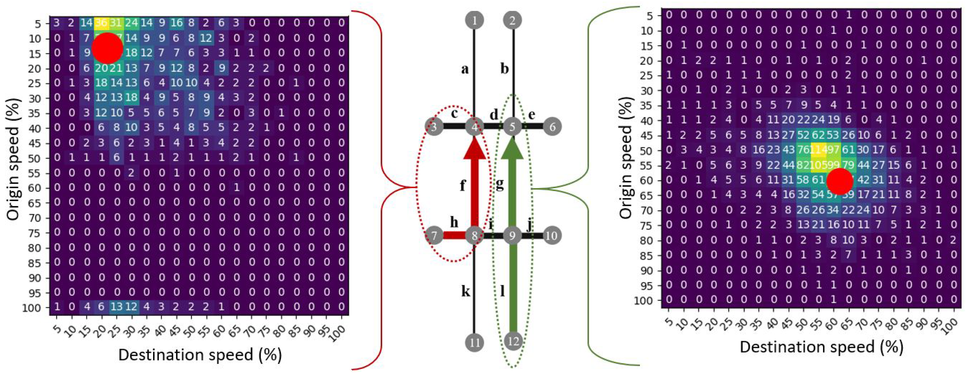
The STM is a novel traffic data representation and modeling technique that captures the vehicle’s speed at the movement between two consecutive road segments called transition [34]. It is used to represent the speed probability change, and therefore it represents the speed probability distribution at one transition in one time interval. The transition is defined as a spatial change in vehicle trajectory when traveling from edge e i to edge e i + 1 in time interval Δ t . As a traffic parameter under observation, the relative harmonic speed is used. The speed is relative to the speed limit on the observed edge. Two examples of the transition are visually represented in Figure 2 with red and green colors. Transitions describe the vehicles that are traveling between edges h f , and l g with corresponding STMs. The STMs represent a very different traffic pattern: (i) On the left-hand side, the traffic congestion with very low origin and destination speeds, and (ii) on the right-hand side, stable traffic flow with origin and destination speeds around 60% of the speed limit. The red circles show the CoM for represented traffic patterns. It can be observed that the position of the CoM is one of the most important parameters when estimating the traffic state, and the next chapters will debate how to use the position of the CoM for anomaly detection.
In this paper, 5% is chosen as the discretization period, and 100% is the maximal possible speed, which resulted in matrix dimensions of 20 × 20. The STM can be represented as:
X ( Δ t ) = p 11 p 12 p 1 n p 21 p m 1 p m n
where p i j represents the probability of transitioning from speed value i to j.

3.3. Tensors

Tensor T is defined as multi-dimensional array T R N 1 × N 2 × × N M , where M represents the order of the tensor (number of dimensions). A vector is then represented with the first-order tensor, matrix with the second-order tensor, and three or more order tensors are called higher-order tensors [35]. For the analysis of the road traffic spatiotemporal data, most authors use a third-order tensor composed using o r i g i n × d e s t i n a t i o n × t i m e and p r o f i l e × r o a d s e g m e n t s × t i m e where profile represents the speed or volume time series on the observed road network segment. Notations and abbreviations are adopted from Kolda and Bader [35].
The decomposition method used in this article is the CANDECOMP/PARAFAC (CP) in its non-negative form. The CP decomposition factorizes a tensor into a sum of component rank-one tensors. For tensor T CP is the following:
T r = 1 R a r b r c r
where R is a positive integer that represents the decomposition rank. Then, rank one components can be expressed as factor matrices A ( a ( 1 ) a ( 2 ) a ( R ) ) , B ( b ( 1 ) b ( 2 ) b ( R ) ) , and C ( c ( 1 ) c ( 2 ) c ( R ) ) .
Most of the authors predefined a tensor rank based on the underlying knowledge of the phenomena that is observed [16]. The Core Consistency Diagnostic (CORCONDIA) [36] method is used in this paper.

4. Methodology

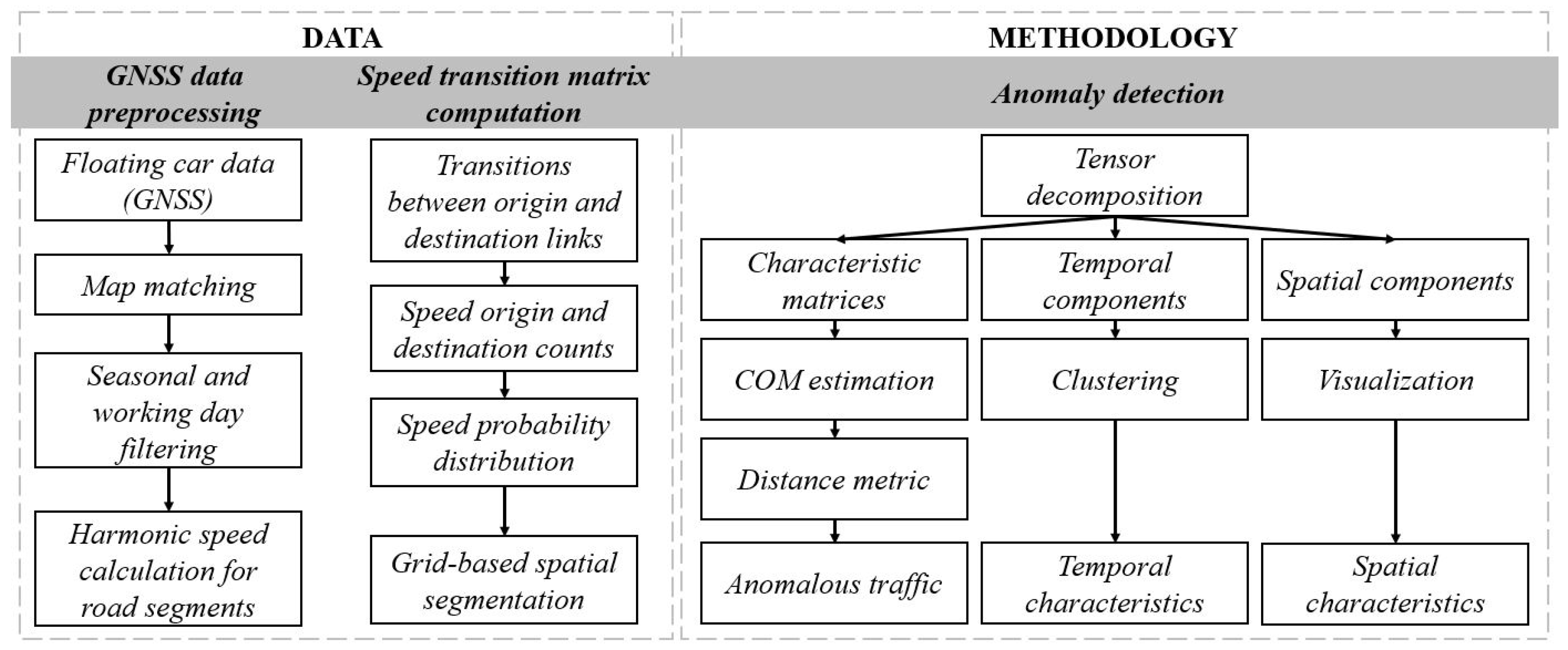
This paper aims to propose a tensor-based road traffic pattern extraction method for the purpose of spatiotemporal anomaly detection. The proposed methodology is presented in Figure 3, and encompasses the main steps: (i) Data preprocessing, (ii) grid-based map segmentation with STMs computation, and (iii) anomaly detection based on the CoM estimation.

4.1. Grid-Based Map Segmentation

When constructing a tensor, many researchers are using one tensor to model the spatiotemporal dataset. In this paper, the goal was to extract many different traffic flow patterns to capture more diverse patterns that are different for many parts of the city. The grid-based map segmentation approach is used to divide the city into many smaller cells. Then, for every cell, all transitions were extracted. The cell’s size was fixed to 500 × 500 m. According to [37], this cell size is sufficient to capture the most important traffic patterns. Transitions were further filtered by discarding every road segment with a speed limit smaller than 50 kmph. This filter was used to avoid any possible false anomaly detection regarding the observed road segments’ low speed or parking lots. There are many different approaches for map segmentation. This approach is used because this paper aims to find and analyze the anomalies on a city-wide scale and give an overview of the city’s most dangerous road segments and possible problems with inadequate traffic signalization.

4.2. Tensor Construction

In this paper, the spatiotemporal tensor composed from the STMs is proposed as a traffic data modeling method. The tensor is constructed by flattening STMs into matrix as a frontal slices, placing transitions as spatial components, and adding time intervals as temporal components, represented in Figure 4. Tensor T R m × n × t is constructed, where m represents the flattened size of the STM, n represents the number of observed transitions in the road network, and t represents eight time intervals. Frontal slices of tensor T can be represented with matrix T : : t R m × n , where every STM matrix X is flattened into a vector x R m × 1 and placed into the matrix T : : t as column. Dimension m had the value of 400 as STM size is 20 × 20 . Instead of using one tensor with all the data, data is divided into several smaller tensors using the grid-based map segmentation, where n represents the number of the transitions inside one grid cell. Then, the final form of the tensors is T ( 1 ) , T ( 2 ) , , T ( N ) where T ( i ) R 400 × n × 8 . With the proposed approach, anomalies can be captured from different parts of the road network, while smaller spatial dimensions of the cells allows capturing more diverse traffic patterns.

4.2.1. Tensor Rank Estimation

In this paper, CORCONDIA is applied as the tensor rank estimation method using the AutoTen algorithm [38]. It is essential to mention that tensor rank estimation methods are used to get recommendations more than the rank’s exact actual value. The algorithm was run five times on randomly chosen tensor T ( i ) , and the average estimated rank resulted in a value of R = 10 , which is the rank used for the experiments.

4.2.2. Factor Matrix Discussion

The tensor decomposition resulted in three factor matrices A R 400 × 10 , B R n × 10 , and C R 8 × 10 as presented in Figure 4. Factor matrix A consists of extracted characteristic traffic patterns on the road network. If the column a : j R 400 × 1 of the factor matrix A is reshaped into the matrix 20 × 20 it represents the characteristic STM (traffic patterns). The goal of anomaly detection is to find the anomalous traffic patterns and link them to the corresponding values in spatial and temporal factor matrices. The matrix B represents the spatial factor matrix, and the values in the rows b i : represent how well each of the characteristic STM represents the traffic flow on the corresponding transition on index i. The values in the columns b : j show how well each characteristic matrix describes each of the transitions (spatial components) in the observed road network. The matrix C represents the temporal factor matrix. The values in the rows c i : represent how well each of the characteristic STM represents the corresponding time interval on index i, and the values in the columns c : j show how well each characteristic matrix describes each of the time interval (temporal components). The larger values in the factor matrices B , and C suggest the greater impact of the spatial or temporal components on the corresponding factor [39].

4.3. Anomaly Detection

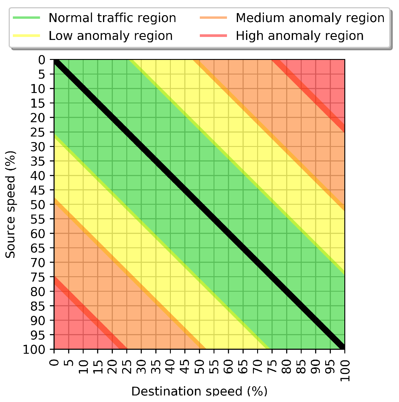
When working with traffic data represented by the STM, the anomalous traffic can be represented by large deviations between origin and destination speeds, which highly depends on the represented pattern’s position. These dangerous traffic situations can be identified by the vehicle’s sudden braking, or a very high acceleration, with the corresponding positions in the STM, lower left, and the upper right corner. Then, normal traffic behavior can be represented if the position of the pattern is close to the diagonal of the STM. Those values represent normal traffic behavior, which extends from the congested (upper left corner) to the free traffic flow (lower right corner). All scenarios are illustrated in Figure 5.
To amplify the importance of the location of the patterns, the method for the anomaly detection is based on (i) CoM estimation for the pattern represented by the characteristic STM, and (ii) measuring the relative distance between CoM and the diagonal of the STM. CoM is computed for every characteristic STM extracted from the tensor decomposition method. With this, extracted CoM represents the most probable speed transition in the characteristic STM. This approach is used because the position of the pattern represented by the STM is crucial for the traffic state estimation and the anomaly detection [40]. CoMs are computed based on the computation of the expected value, adopted from [41]. Firstly, marginal distribution for the coordinates (origin and destination speed) are computed using Equations (3) and (4):
p x ( x j ) = i = 1 m p i j , j = 1 , 2 , , n ,
p y ( y i ) = j = 1 n p i j , i = 1 , 2 , , n ,
where p x ( x j ) and p y ( y i ) represent the marginal distributions for the coordinates. Then, the CoM coordinates are computed using:
c x = j = 1 n p x ( x j ) · j ,
c y = i = 1 m p y ( y i ) · i ,
where c x and c y represent coordinates of the CoM.
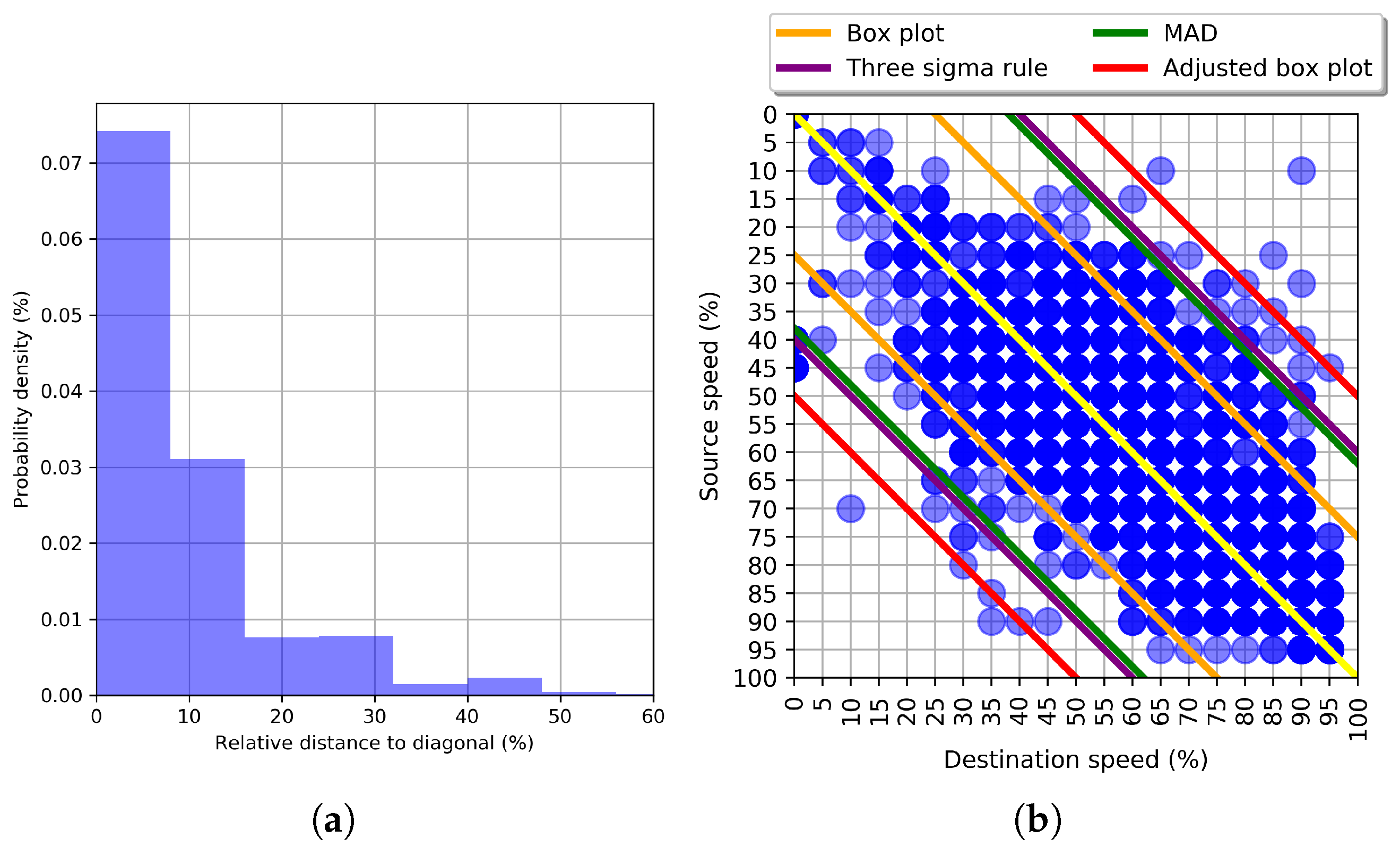
After the CoM estimation, the relative distance between the CoM and the diagonal is measured using the Euclidean distance. The most suitable anomaly detection method is chosen by comparison of the most used methods represented in Table 1, that reports the name of the anomaly detection method, number of anomalies detected, and the lower and upper bounds. Relative distance from the diagonal values that are placed outside of the computed bounds are considered as anomalous ones. The box plot method resulted in detecting the most anomalies, three sigma rule, and MAD resulted in detecting the same amount of anomalies, while, adjusted box plot detected eight anomalous characteristic matrices. After examining the relative distance distribution (Figure 6a), the adjusted box plot is chosen as an anomaly detection method. It is a method that does not take any parametric assumptions and uses med couple as a robust skewness estimator [42]. Other methods assume the normal distribution of the data and cannot be used in this case. The results of applying all the methods can be observed in Figure 6b, where the plotted lines show the upper bound of the anomaly detection methods with plotted CoMs for every calculated characteristic STM resulted in tensor decomposition. It can be observed that the adjusted box plot resulted in detecting only the most anomalous transitions regarding the anomaly definition presented in Section 3.1.
The tensor-based anomaly detection method is presented in Algorithm 1. The algorithm begins with the empty lists initialization, namely, list of tensors T and the list of anomalous characteristic matrices M . Every tensor T ( i ) is constructed by flattening every STM recorded inside the spatial cell g ( i ) G , and constructing a frontal slice T : : t explained in detail in Section 4.2. Then, on every tensor, the Non-negative Tensor Decomposition (NTD) is applied to compute three factor matrices. A i represents extracted traffic patterns, where every row a : i represent flattened extracted characteristic matrix, B i spatial factor matrix, and C i temporal factor matrix. Then, every a : i is reshaped into two dimensional STM X c h ( i ) and CoM coordinates are computed using Equations (3)–(6). The final step is the anomaly detection, which is estimated by using two distances d C o M and d A , where d C o M represents the distance from the CoM to the diagonal of the STM, and d A threshold distance for the anomaly detection visually shown in Figure 6. The anomaly is detected if the d C o M is larger or equal than the d A and placed into list M .
Algorithm 1 Tensor-based anomaly detection pseudo code
 Input: Spatial cells G, STMs
1:
Initialize empty list of tensors T
2:
Initialize empty list of anomalous characteristic matrices M
3:
for each spatial cell g ( i ) in G do
4:
   Construct a new tensor T ( i ) R m × n × t using STMs for cell g ( i )
5:
   Add new tensor T ( i ) to list T
6:
end for
7:
for each tensor T ( i ) in list T  do
8:
   Apply Non-negative Tensor Decomposition on T ( i ) and store the result in matrices A i , B i and C i
9:
   for each flattened characteristic matrix a : i in A i  do
10:
     Reshape matrix a : i to 20 × 20 matrix and set it as X c h ( i )
11:
     Compute CoM coordinates c x ( i ) and c y ( i ) from X c h ( i )
12:
     Compute distance d C o M between CoM coordinates and the diagonal of X c h ( i )
13:
     if  d C o M d A  then
14:
        Add X c h ( i ) to list M
15:
     end if
16:
   end for
17:
end for

5. Results

5.1. Data

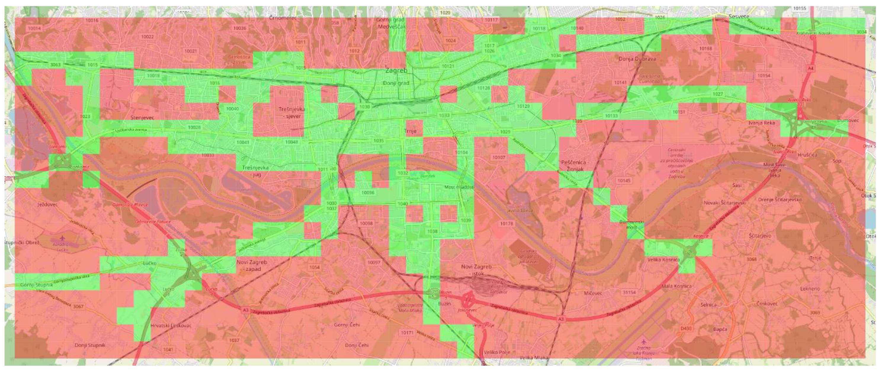
A real-life dataset was provided by the Mireo Inc. from Zagreb, Croatia [43]. It consists of large GNSS data collected between 2009 and 2014 by vehicle fleet with the size of approximately 5000 vehicles (Table 2). The dataset includes around 6.55 billion GNSS records driven across all Croatia. For this paper, the dataset is filtered to represent data for the City of Zagreb, as a mid-size city in the European context with a population of around 800,000 people. To lower deviations due to the road traffic seasonality issue [44], weekend days, the summer months, July, and August are excluded from the dataset. The grid-based map segmentation and the filtering were applied to the dataset, and the results are shown in Figure 7, where green represents the cell with the data, and red cells are excluded from this research.

5.2. Anomalous Traffic Patterns

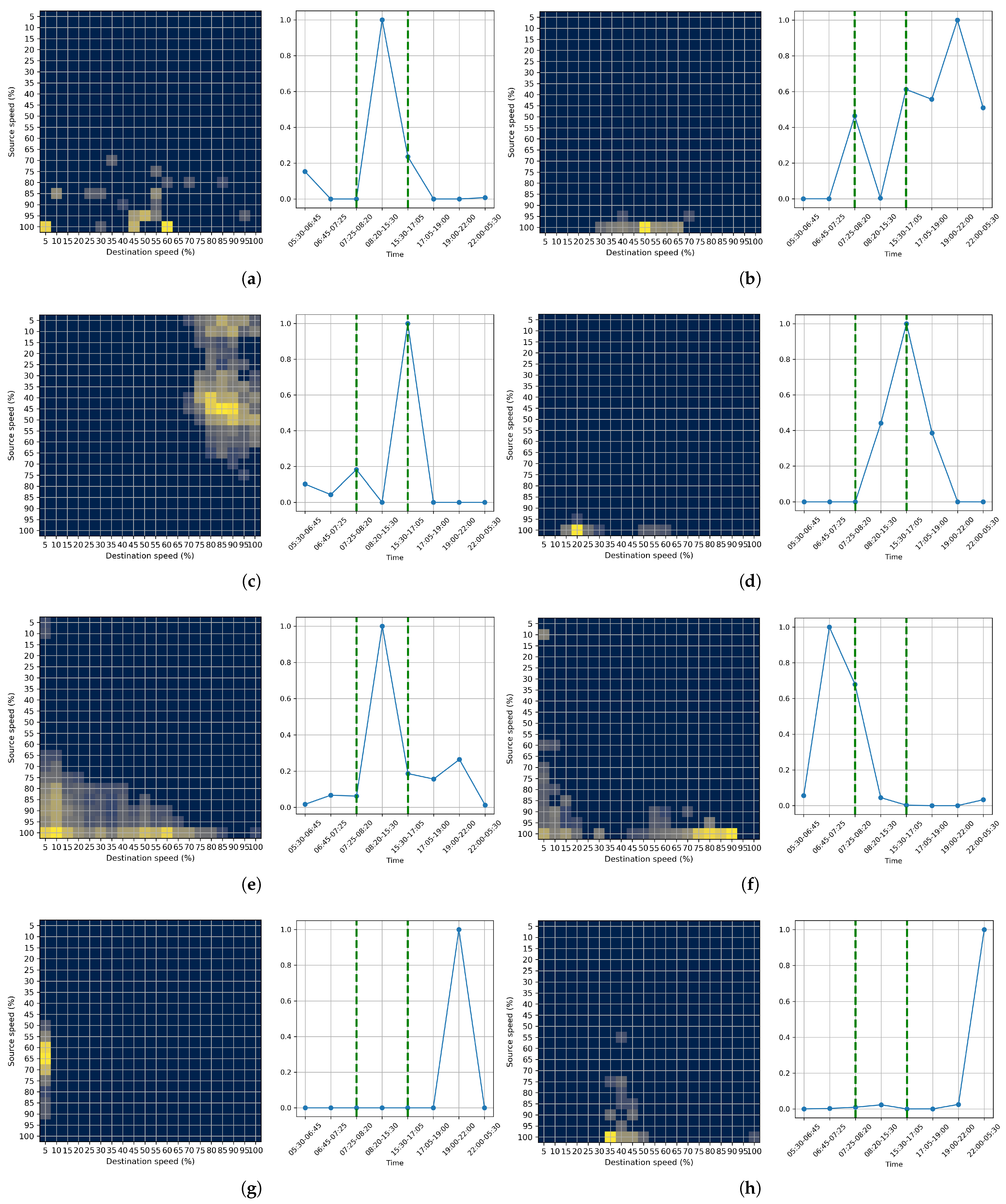
This section shows the evaluation results using the real-life dataset. Figure 8 presents eight extracted characteristic matrices, with corresponding temporal components, in which the morning (07:25–08:20) and evening (15:30–17:05) rush hours are labeled with striped green lines. Figure 9 represents the spatial placement of the extracted anomalous cells, where every anomaly event is labeled with a letter that corresponds to the Figure 8 labels.
All characteristic matrices, except for (c) example, represent the same anomaly type as the CoM placed at the matrix’s lower-left corner. This traffic situation is characterized by sudden brakes and large speed decrease when traveling from origin to destination links. These situations occur when a vehicle is facing congestion ahead and represent a potentially serious safety threat. The (c) example is the opposite situation, where the CoM is placed in the upper right corner. Here, a different but potentially dangerous event occurs, where vehicles are accelerating from low to very high speeds.
Most of the temporal components indicate that anomalous events occur at rush hours. It can be observed that the period between rush hours (08:20–15:30) and the evening rush hour is the most represented case. This claim is justified because in rush hours, many vehicles are on the roads, and the anomaly probability arises.
Figure 9 represents the spatial placement of the extracted abnormal cells, where every anomaly event is labeled with a letter that corresponds to the labels in Figure 8. The spatial placement of the anomalies indicates two spatial clusters: (i) Edges of the city represented with the examples (a), (b), (d), (f), (h), and (ii) city center represented with the examples (c), (e), and (g). The cluster of transitions placed at the edges of the city points to the congestion related to daily commuters traveling to work from outside of the city center. By considering temporal components, it can be observed that the evening rush hour contributes mostly to the congestion and the anomalous events in the city, with the exception of example (f), where the anomalous events mostly occur at the morning rush hour. The city center cluster is characterized by the temporal components that point to the intervals between rush hours, evening rush hour, and the interval later in the day, after the evening rush hour. This behavior is mostly attributed to the inefficient traffic signalization, which leads to the prolongation of the anomaly events mostly caused by the rush-hour congestion. Similar behavior can be caused by the tourist attractions and other entertainment facilities provided at the city center. During the transition in example (e), the most congested bridge in the city was captured. This information indicates the possible usable information for the urban planners by suggesting the need to build a new bridge that will connect the north and the south parts of the city.

5.3. Domain Knowledge Validation

The HCM provides methods for computing relevant traffic parameters to estimate the capacity and the level of service for different road types [45]. Level of service is defined using a relative traffic flow speed on the observed road segments, labeled with letters from A to F, where A represents the best traffic conditions, with vehicle speeds larger than 80% of the free-flow speed, and F represents the most extreme congestion, where vehicle speeds are less than 30% of the free-flow speed. The 2000 STMs were labeled using the HCM data for the level of service. STMs were labeled as anomalous only if the transition contains a significant change in the level of service, i.e., from A to F, or from F to A. With this setup, the recurrent congestion was not detected as an anomaly. In other cases, STMs were labeled as normal. With this setting, only most extreme anomalies were labeled as abnormal. Firstly, 500 anomalous and 500 STMs without the anomaly were selected randomly from the labeled data as a training dataset. Then the results of our approach were compared to the HCM classification as the ground truth. We report the precision calculated as t r u e p o s i t i v e / ( t r u e p o s i t i v e + f a l s e p o s i t i v e ) , recall as t r u e p o s i t i v e / ( t r u e p o s i t i v e + f a l s e n e g a t i v e ) , and F-1 score in Table 3.

5.4. Comparison to Other Approaches

This section compares the proposed approach to other approaches for road traffic anomaly detection. While there are many tensor-based approaches focused on congestion estimation, missing data imputation, and event detection, there are only a few specialized in anomaly detection on urban roads. Table 4 shows several tensor-based approaches for the anomaly detection of road traffic networks. Most of the authors are using O-D matrices that show the number of the vehicle (volume) traveling between two points in the traffic network [9,18,46]. Regarding the potentially large spatial distance between the O-D pairs, those approaches extract the patterns and detect global anomalies related to traffic fluctuations [47]. Therefore, most of the authors focus on the detection of the general events that are related to traffic movements like tourist attractions or other social events [46,48].
This paper focuses on detecting the anomalies that affect the traffic flow on micro-locations (transitions). The proposed approach is more suitable for detecting anomalies that could potentially lead to traffic accidents like sudden braking or fast acceleration. Therefore, this approach can be applied in real-time traffic accident detection and prediction.
Alongside the possible applications of the proposed methodology, some drawbacks of the method must be addressed in the further research. The anomaly detection method is based on the speed, which can be lead to false anomaly detection on a short road segments bounded with the non-synchronised intersections. This is the reason why the short road segments with the speed limit less than 50 kmph was excluded from this research. Secondly, more narrow time intervals like 5-, 15-, or 30 min are used in most of the road traffic related research. Narrower time intervals could provide more informative results with the possibilities of implementing the method on a real-time case study especially in the environment with the mixed traffic flows [49]. Further improvements of the method could also include the analysis of the interactions between the consecutive cells. The modeling process of the STM should also be addressed. The important parameters of the STM like size, discretization period, and cell size should be analyzed for optimization purposes.

6. Conclusions

For the development of the more secure, cleaner, and overall more sustainable cities, traffic congestion and corresponding anomalies must be addressed. This paper presents a novel method for the extraction of road traffic patterns and anomaly detection using tensor-based method. It integrates a tensor decomposition with the anomaly detection approach based on estimating the CoM of the observed traffic pattern represented by the STM. This method is evaluated on a large real-life GNSS road traffic dataset and validated using the domain knowledge data. The result presents the valuable traffic insights useful for the routing application, responsible urban planners, and road infrastructure maintenance authorities. It can be used as valuable traffic information about the need for infrastructure expansion, additional improvement strategies, or to analyze the traffic influence of the new road infrastructure.
Compared to other approaches related to road traffic anomaly detection, the proposed method is more focused on detecting the anomalies that affect the traffic flow and could lead to dangerous situations and, consequently, to traffic accidents. Furthermore, anomaly detection will include the expansion of the proposed method for the real-time anomaly detection framework.

Author Contributions

Conceptualization, L.T. and T.C.; methodology, L.T., S.F. and J.G.; software, L.T.; validation, L.T. and T.C.; formal analysis, L.T.; investigation, L.T.; resources, T.C.; data curation, L.T. and T.C.; writing—original draft preparation, L.T. and S.F.; writing—review and editing, L.T., S.F., T.C. and J.G.; visualization, L.T.; supervision, T.C. and J.G.; project administration, T.C.; funding acquisition, T.C. All authors have read and agreed to the published version of the manuscript.

Funding

This research was funded by European Regional Development Fund under the grant KK.01.1.1.01.0009 (DATACROSS). Sofia Fernandes acknowledges the support of FCT (Fundação para a Ciência e a Tecnologia) via the Ph.D. scholarship PD/BD/114189/2016.

Acknowledgments

The data used for this research was collected during the project SORDITO, European Regional Development Fund under contract RC.2.2.08-0022. This work has been partly supported by the University of Zagreb and the Faculty of Transport and Traffic Sciences under the grant “Innovative Models and Control Strategies for Sustainable Mobility in Smart Cities” and “Optimization of the Line Transport Timetables for the Case of Electric Vehicles: A Proof of Concept”.

Conflicts of Interest

The authors declare no conflict of interest.

Abbreviations

The following abbreviations are used in this manuscript:
CoMCenter of Mass
CORCONDIACore Consistency Diagnostic
CPCANDECOMP/PARAFAC
GNSSGlobal Navigation Satellite System
HCMHighway Capacity Manual
ITSIntelligent Transport Systems
NTDNon-negative Tensor Decomposition
O-DOrigin-Destination
PCAPrincipal Components Analysis
STMSpeed Transition Matrix

References

  1. Li, D.; Yang, M.; Jin, C.J.; Ren, G.; Liu, X.; Liu, H. Multi-Modal Combined Route Choice Modeling in the MaaS Age Considering Generalized Path Overlapping Problem. IEEE Trans. Intell. Transp. Syst. 2021, 22, 2430–2441. [Google Scholar] [CrossRef]
  2. Tišljarić, L.; Fernandes, S.; Carić, T.; Gama, J. Spatiotemporal Traffic Anomaly Detection on Urban Road Network Using Tensor Decomposition Method. In Discovery Science; Appice, A., Tsoumakas, G., Manolopoulos, Y., Matwin, S., Eds.; Springer International Publishing: Cham, Switzerland, 2020; pp. 674–688. [Google Scholar]
  3. Erdelić, T.; Ravlić, M.; Carić, T. Travel time prediction using speed profiles for road network of Croatia. In Proceedings of the International Symposium ELMAR, Zadar, Croatia, 12–14 September 2016; pp. 97–100. [Google Scholar] [CrossRef]
  4. Ma, X.; Dai, Z.; He, Z.; Ma, J.; Wang, Y.; Wang, Y. Learning traffic as images: A deep convolutional neural network for large-scale transportation network speed prediction. Sensors 2017, 17, 818. [Google Scholar] [CrossRef] [Green Version]
  5. Nguyen, H.; Liu, W.; Chen, F. Discovering Congestion Propagation Patterns in Spatio-Temporal Traffic Data. IEEE Trans. Big Data 2017, 3, 169–180. [Google Scholar] [CrossRef]
  6. Zhang, H.; Wu, Y.; Tan, H.; Dong, H.; Ding, F.; Ran, B. Understanding and Modeling Urban Mobility Dynamics via Disentangled Representation Learning. IEEE Trans. Intell. Transp. Syst. 2020, 1–11. [Google Scholar] [CrossRef]
  7. Zhang, B.; Chen, S.; Ma, Y.; Li, T.; Tang, K. Analysis on spatiotemporal urban mobility based on online car-hailing data. J. Transp. Geogr. 2020, 82, 102568. [Google Scholar] [CrossRef]
  8. Wang, Z.; Hu, K.; Xu, K.; Yin, B.; Dong, X. Structural analysis of network traffic matrix via relaxed principal component pursuit. Comput. Netw. 2012, 56, 2049–2067. [Google Scholar] [CrossRef] [Green Version]
  9. Fanaee-T, H.; Gama, J. Event detection from traffic tensors: A hybrid model. Neurocomputing 2016, 203, 22–33. [Google Scholar] [CrossRef] [Green Version]
  10. Xu, G.; Khan, S.; Zhu, H.; Han, L.; Ng, M.K.; Yan, H. Discriminative tracking via supervised tensor learning. Neurocomputing 2018, 315, 33–47. [Google Scholar] [CrossRef]
  11. Rendle, S. Factorization Machines with LibFM. ACM Trans. Intell. Syst. Technol. 2012, 3, 57. [Google Scholar] [CrossRef]
  12. Prada, M.A.; Dominguez, M.; Barrientos, P.; Garcia, S. Dimensionality Reduction for Damage Detection in Engineering Structures. Int. J. Mod. Phys. B 2012, 26, 1246004. [Google Scholar] [CrossRef]
  13. Tian, X.; Zhang, X.; Deng, X.; Chen, S. Multiway kernel independent component analysis based on feature samples for batch process monitoring. Neurocomputing 2009, 72, 1584–1596. [Google Scholar] [CrossRef]
  14. Fanaee-T, H.; Gama, J. EigenEvent: An Algorithm for Event Detection from Complex Data Streams in Syndromic Surveillance. Intell. Data Anal. 2015, 19, 597–616. [Google Scholar] [CrossRef] [Green Version]
  15. Gauvin, L.; Panisson, A.; Cattuto, C. Detecting the Community Structure and Activity Patterns of Temporal Networks: A Non-Negative Tensor Factorization Approach. PLoS ONE 2014, 9, e86028. [Google Scholar] [CrossRef] [PubMed] [Green Version]
  16. Wang, J.; Gao, F.; Cui, P.; Li, C.; Xiong, Z. Discovering Urban Spatio-temporal Structure from Time-Evolving Traffic Networks. In Web Technologies and Applications; Chen, L., Jia, Y., Sellis, T., Liu, G., Eds.; Springer International Publishing: Cham, Switzerland, 2014; pp. 93–104. [Google Scholar]
  17. Fernandes, S.; Fanaee-T, H.; Gama, J.; Tišljarić, L.; Šmuc, T. WINTENDED: WINdowed TENsor decomposition for Densification Event Detection in time-evolving networks. Mach. Learn. 2020. [Google Scholar] [CrossRef]
  18. Wang, X.; Fagette, A.; Sartelet, P.; Sun, L. A Probabilistic Tensor Factorization Approach to Detect Anomalies in Spatiotemporal Traffic Activities. In Proceedings of the IEEE Intelligent Transportation Systems Conference, Auckland, New Zealand, 27–30 October 2019; pp. 1658–1663. [Google Scholar] [CrossRef]
  19. Tang, K.; Chen, S.; Liu, Z. Citywide spatial-temporal travel time estimation using big and sparse trajectories. IEEE Trans. Intell. Transp. Syst. 2018, 19, 4023–4034. [Google Scholar] [CrossRef]
  20. Tan, H.; Yang, Z.; Feng, G.; Wang, W.; Ran, B. Correlation Analysis for Tensor-based Traffic Data Imputation Method. Procedia Soc. Behav. Sci. 2013, 96, 2611–2620. [Google Scholar] [CrossRef] [Green Version]
  21. Tan, H.; Wu, Y.; Shen, B.; Jin, P.J.; Ran, B. Short-Term Traffic Prediction Based on Dynamic Tensor Completion. IEEE Trans. Intell. Transp. Syst. 2016, 17, 2123–2133. [Google Scholar] [CrossRef]
  22. Pan, P.; Wang, H.; Li, L.; Wang, Y.; Jin, Y. Peak-Hour Subway Passenger Flow Forecasting: A Tensor Based Approach. In Proceedings of the 21st International Conference on Intelligent Transportation Systems, Maui, HI, USA, 4–7 November 2018; pp. 3730–3735. [Google Scholar] [CrossRef]
  23. Chen, X.; He, Z.; Chen, Y.; Lu, Y.; Wang, J. Missing traffic data imputation and pattern discovery with a Bayesian augmented tensor factorization model. Transp. Res. Part Emerg. Technol. 2019, 104, 66–77. [Google Scholar] [CrossRef]
  24. Chandola, V. Anomaly Detection: A Survey. ACM Comput. Surv. 2009, 41, 15. [Google Scholar] [CrossRef]
  25. Schubert, E.; Zimek, A.; Kriegel, H.P. Local outlier detection reconsidered: A generalized view on locality with applications to spatial, video, and network outlier detection. Data Min. Knowl. Discov. 2014, 28, 190–237. [Google Scholar] [CrossRef]
  26. Feng, Z.; Zhu, Y. A Survey on Trajectory Data Mining: Techniques and Applications. IEEE Access 2016, 4, 2056–2067. [Google Scholar] [CrossRef]
  27. Zheng, Y. Trajectory Data Mining: An Overview. ACM Trans. Intell. Syst. Technol. 2015, 6, 29:1–29:41. [Google Scholar] [CrossRef]
  28. Gupta, M.; Gao, J.; Aggarwal, C.C.; Han, J. Outlier Detection for Temporal Data: A Survey. IEEE Trans. Knowl. Data Eng. 2014, 26, 2250–2267. [Google Scholar] [CrossRef]
  29. Djenouri, Y.; Belhadi, A.; Lin, J.C.w.; Djenouri, D.; Cano, A. A Survey on Urban Traffic Anomalies Detection Algorithms. IEEE Access 2019, 7, 12192–12205. [Google Scholar] [CrossRef]
  30. Tan, P.N.; Steinbach, M.; Kumar, V. Anomaly Detection. In Introduction to Data Mining, 2nd ed.; Pearson Addison Wesley: Boston, MA, USA, 2006; pp. 651–684. [Google Scholar]
  31. Guo, J.; Huang, W.; Williams, B.M. Real time traffic flow outlier detection using short-term traffic conditional variance prediction. Transp. Res. Part C Emerg. Technol. 2014, 50, 160–172. [Google Scholar] [CrossRef]
  32. Pan, B.; Zheng, Y.; Wilkie, D.; Shahabi, C. Crowd Sensing of Traffic Anomalies Based on Human Mobility and Social Media. In Proceedings of the 21st ACM SIGSPATIAL International Conference on Advances in Geographic Information Systems, Orlando, FL, USA, 5–8 November 2013; pp. 344–353. [Google Scholar] [CrossRef] [Green Version]
  33. Chen, S.; Wang, W.; Zuylen, H.V. A comparison of outlier detection algorithms for ITS data. Expert Syst. Appl. 2010, 37, 1169–1178. [Google Scholar] [CrossRef]
  34. Tišljarić, L.; Ivanjko, E.; Kavran, Z.; Carić, T. Fuzzy Inference System for Congestion Index Estimation Based on Speed Probability Distributions. Trans. Res. Proc. 2021, 55, 2021. [Google Scholar] [CrossRef]
  35. Kolda, T.G.; Bader, B.W. Tensor decompositions and applications. SIAM Rev. 2009, 51, 455–500. [Google Scholar] [CrossRef]
  36. Bro, R.; Kiers, H.A.L. A new efficient method for determining the number of components in PARAFAC models. J. Chemom. 2003, 17, 274–286. [Google Scholar] [CrossRef]
  37. Carić, T.; Fosin, J. Using Congestion Zones for Solving the Time Dependent Vehicle Routing Problem. Promet-Traffic Transp. 2020, 32, 25–38. [Google Scholar] [CrossRef]
  38. Papalexakis, E.E. Automatic Unsupervised Tensor Mining with Quality Assessment. In Proceedings of the International Conference on Data Mining, Miami, FL, USA, 5–7 May 2016; pp. 711–719. [Google Scholar] [CrossRef] [Green Version]
  39. Qi, G.; Huang, A.; Guan, W.; Fan, L. Analysis and Prediction of Regional Mobility Patterns of Bus Travellers Using Smart Card Data and Points of Interest Data. IEEE Trans. Intell. Transp. Syst. 2019, 20, 1197–1214. [Google Scholar] [CrossRef]
  40. Tišljarić, L.; Carić, T.; Abramović, B.; Fratrović, T. Traffic State Estimation and Classification on Citywide Scale Using Speed Transition Matrices. Sustainability 2020, 12, 7278. [Google Scholar] [CrossRef]
  41. Jordaan, I.J. Decisions under Uncertainty: Probabilistic Analysis for Engineering Decisions; Cambridge University Press: Cambridge, UK, 2005; pp. 127–144. [Google Scholar]
  42. Hubert, M.; Vandervieren, E. An adjusted boxplot for skewed distributions. Comput. Stat. Data Anal. 2008, 52, 5186–5201. [Google Scholar] [CrossRef]
  43. Erdelić, T.; Ravlić, M. SORDITO—System for Route Optimization in Dynamic Transport Environment. Promet-Traffic Transp. 2016, 28, 193–194. [Google Scholar] [CrossRef] [Green Version]
  44. Capparuccini, D.M.; Faghri, A.; Polus, A.; Suarez, R.E. Fluctuation and Seasonality of Hourly Traffic and Accuracy of Design Hourly Volume Estimates. Transp. Res. Rec. 2008, 2049, 63–70. [Google Scholar] [CrossRef]
  45. HCM2010. Highway Capacity Manual; Transportation Research Board, National Research Council: Washington, DC, USA, 2010. [Google Scholar]
  46. Lin, C.; Zhu, Q.; Guo, S.; Jin, Z.; Lin, Y.R.; Cao, N. Anomaly detection in spatiotemporal data via regularized non-negative tensor analysis. Data Min. Knowl. Discov. 2018, 32, 1056–1073. [Google Scholar] [CrossRef] [Green Version]
  47. Lykov, S.; Asakura, Y. Anomalous Traffic Pattern Detection in Large Urban Areas: Tensor-Based Approach with Continuum Modeling of Traffic Flow. Int. J. Intell. Transp. Syst. Res. 2018, 18, 13–21. [Google Scholar] [CrossRef]
  48. Chen, L.; Jakubowicz, J.; Yang, D.; Zhang, D.; Pan, G. Fine-Grained Urban Event Detection and Characterization Based on Tensor Cofactorization. IEEE Trans. Hum.-Mach. Syst. 2017, 47, 380–391. [Google Scholar] [CrossRef]
  49. Vrbanić, F.; Ivanjko, E.; Kušić, K.; Čakija, D. Variable Speed Limit and Ramp Metering for Mixed Traffic Flows: A Review and Open Questions. Appl. Sci. 2021, 11, 2574. [Google Scholar] [CrossRef]
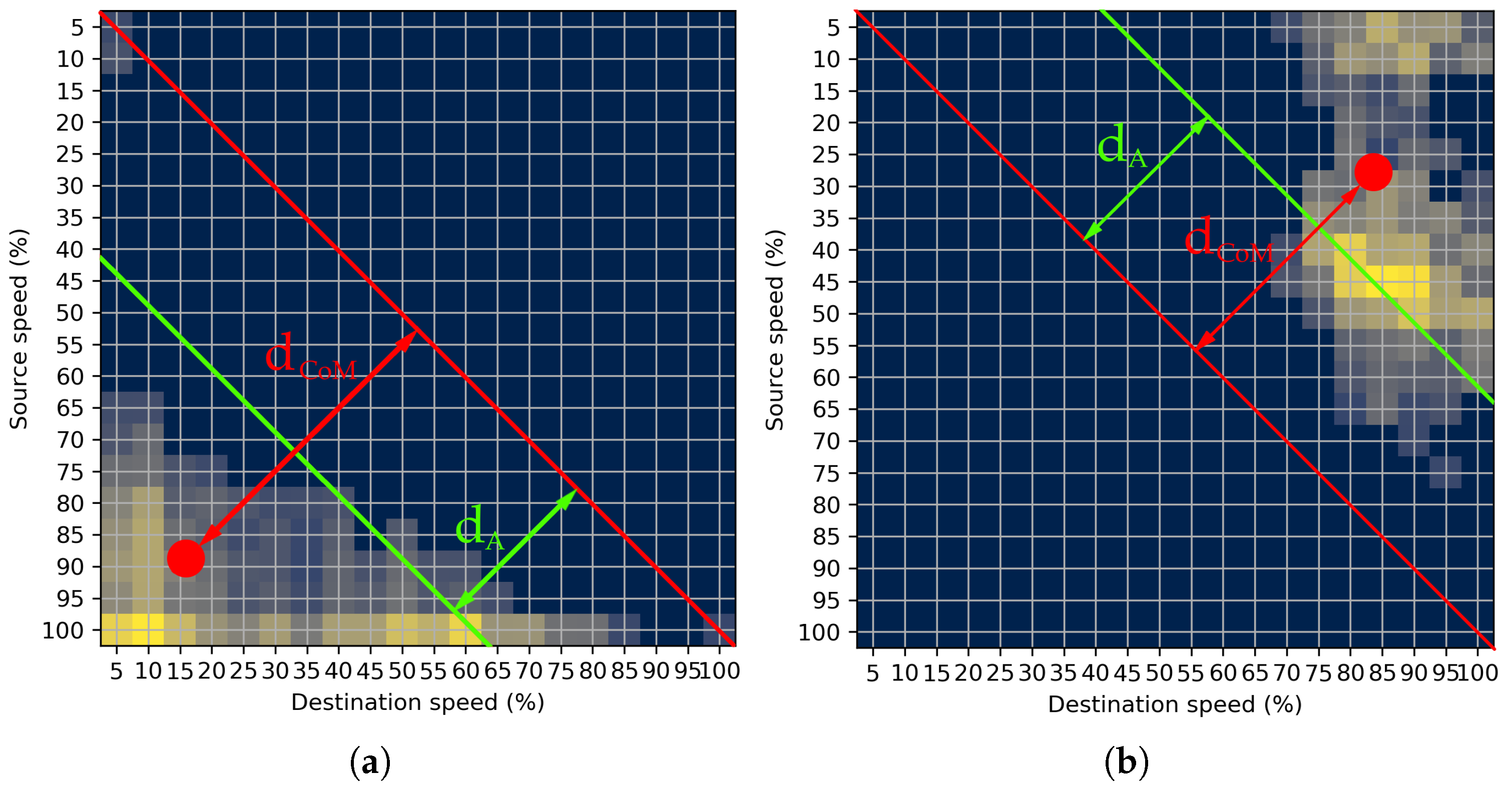
Figure 1. Example of two possible anomaly types: (a) Sudden breaks and (b) intense accelerations.
Applsci 11 12017 g001
Figure 2. Transitions (center), congested STM (left), and normal traffic STM (right) examples on a simple road network.
Applsci 11 12017 g002
Figure 3. Proposed methodology for the anomaly detection.
Applsci 11 12017 g003
Figure 4. Steps that are describing the tensor construction method using the STMs: (1) Grid-based map segmentation, (2) STM extraction, (3) tensor construction, and (4) factor matrices.
Applsci 11 12017 g004
Figure 5. Regions in the STM that shows pattern location importance for anomaly detection.
Applsci 11 12017 g005
Figure 6. Choosing the anomaly detection method: (a) Distribution of the relative distances to the diagonal of the STM, and (b) CoMs of the characteristic matrices with labeled anomaly measures results.
Applsci 11 12017 g006
Figure 7. Result of the grid-based map segmentation and the data filtering process.
Applsci 11 12017 g007
Figure 8. Results of the anomaly detection; (ah) represent characteristic matrices which represent anomalous patterns (left) with corresponding temporal components (right).
Applsci 11 12017 g008
Figure 9. Positions of the anomalous cells on the map (ah) represent most anomalous parts of the traffic network in the City of Zagreb.
Applsci 11 12017 g009
Table 1. Comparison of the multiple anomaly detection methods.
MethodN. Anomalies DetectedBounds
Box plot261 [ 15.00 , 25.00 ]
Three sigma rule58 [ 20.12 , 39.13 ]
MAD58 [ 24.38 , 38.52 ]
Adjusted Box plot8 [ 4.65 , 46.13 ]
Table 2. Data summary.
Number of GNSS traces6.55 billion
Sampling rate100 m/5 min
Time-spanAugust 2008–October 2014
Number of vehicles4200
Number of road segments (Croatia)2,000,000
Number of road segments (Zagreb)86,900
Table 3. Validation results of the proposed method by using the domain knowledge data.
Anomalous STMsNormal STMsPrecisionRecallF-1
500500 92.88 % 87.55 % 90.14%
Table 4. Comparison of the proposed approach to other approaches for the traffic anomaly detection.
LiteratureData TypeTraffic ParameterAnomaly Detection
Fanaee et al. [9]O-D matrices (car)Traffic volumeTraffic flow or topology
Wang et al. [18]O-D matrices (car)Traffic volumeTraffic Flow
Lin et al. [46]O-D matrices (car)Traffic volumeEvent detection
Chen et al. [48]GNSS (bicycle)Traffic volumeEvent detection
Lykov et al. [47]Simulation (car)Traffic speedTraffic patterns
Publisher’s Note: MDPI stays neutral with regard to jurisdictional claims in published maps and institutional affiliations.