UAVC: A New Method for Correcting Lidar Overlap Factors Based on Unmanned Aerial Vehicle Vertical Detection

Abstract

A method to calibrate the overlap factor of Lidar is proposed, named unmanned aerial vehicle correction (UAVC), which uses unmanned aerial vehicles (UAVs) to detect the vertical distribution of particle concentrations. The conversion relationship between the particulate matter concentration and the aerosol extinction coefficient is inverted by the high-altitude coincidence of the vertical detection profiles of the UAV and Lidar. Using this conversion relationship, the Lidar signal without the influence of the overlap factor can be inverted. Then, the overlap factor profile is obtained by comparing the signal with the original Lidar signal. A 355 nm Raman-Mie Lidar and UAV were used to measure overlap factors under different weather conditions. After comparison with the Raman method, it is found that the overlap factors calculated by the two methods are in good agreement. The changing trend of the extinction coefficient at each height is relatively consistent, after comparing the inversion result of the corrected Lidar signal with the ground data. The results show that after the continuously measured Lidar signal is corrected by the overlap factor measured by this method, low-altitude aerosol information can be effectively obtained.

1. Introduction

Aerosols with the ability to reflect, absorb, and scatter light are composed of solid or liquid particles suspended in the atmosphere. Generally, climate change will be directly or indirectly affected by aerosols [1,2,3,4]. It will also have a serious impact on human health, especially the respiratory system [5,6]. On the other hand, aerosols will reduce atmospheric visibility, which will have an important impact on traffic, navigation, and satellite remote sensing [7,8]. In recent years, the globalization process has become inseparable from the excessive combustion of fossil fuels and automobile exhaust emissions, and anthropogenic aerosol pollution in many areas has become increasingly serious [9,10,11]. Lidar is an important tool for detecting the spatial and temporal distribution of aerosols and is widely used in the fields of atmospheric science research and environmental monitoring [12,13,14,15]. However, for Lidar low-altitude observations, the incomplete overlap of the laser beam and the telescope’s field of view (FOV) in the near field partially receive the echo signal. The ratio of the overlap area to the cross-section of the laser beam is called the overlap factor or geometrical form factor [16]. To effectively detect the vertical distribution of low-altitude aerosols, the overlap factor of Lidar must be corrected. The overlap factor is zero in the near field and gradually reaches one as the distance increases. The influenced distance of the overlap factor differs from a few hundred meters to three kilometers, depending on the structure of the transmitting and receiving systems. Theoretically, the overlap factor can be calculated by a ray-tracing model [17,18]. In practice, the system parameters are difficult to obtain accurately, so the overlap factors are mainly obtained by experimental means. For example, Y. Sasano et al. proposed that the overlap factor can be obtained through horizontal observations under the condition of a uniform atmospheric level [19]. Wandinger et al. proposed a method of using Raman signals to measure overlap factors [20]. In recent years, the traditional Raman method has been improved by the introduction of constraints by researchers [21,22,23]. It is worth noting that for aerosol Lidar that cannot perform horizontal observation and only has a meter scattering channel, the horizontal observation method and the Raman method are not suitable for calculating overlap factors. Therefore, Guerrero Rascado et al. combined the ceilometer profile to extract the overlap factors of the Lidar [24]. Z. Wang et al. used CCD to observe the side scattering of the emitted beam to calculate the overlap factor [25]. However, to meet the detection accuracy requirements of more Lidar in different complex environments, more methods for correcting the overlap factor need to be studied.

In this paper, a method to correct the overlap factor of Lidar is proposed, named UAVC (unmanned aerial vehicle correction), which uses an aerial vehicle (UAV) to detect the vertical distribution of particle concentration. In Section 2, the experiment and method are introduced. In Section 3, the overlap factor of the two methods under different weather conditions is calculated. The low-altitude detection capabilities of Lidar before and after geometric factor correction are compared. Finally, a conclusion is given in Section 4.

2. Experiment and Method

A Raman-Mie Lidar (model: LR112-D400, Raymetrics S.A., Athens, Greece) and a six-rotor UAV (model: M6E, Tiantu Aviation Technology Co. Ltd., Beijing, China) equipped with light scattering particle detectors (are the main instruments of the experiment. The Raman-Mie Lidar emission wavelength is 355 nm, and the system parameters are shown in

Table 1. The parameters of Raman-Mie Lidar.

Parameters	Values
Transmitter
Transmitted wavelength	355 nm
Pulse energy	50 mJ
Pulse repetition rate	10 Hz
Pulse duration	8 ns
Laser beam divergence	0.2 mrad
Receiver
Telescope diameter	400 mm
FOV	0.5–2 mrad
Detect channels	355, 387, 408
Filter bandwidth	1 nm
Data acquisition
Sample rate	40 MHz
Resolution	12 bit

. The 355 nm elastic scattering signal, the 387 nm nitrogen Raman scattering signal, and the 408 nm water vapour Raman scattering signal are simultaneously received by the Cassegrain telescope. The Lidar only works in the vertical state and has the ability to detect Raman signals at night. The acquired Raman signal is used to calculate the overlap factor for comparison with the method proposed in this paper.

An M6E six-rotor UAV produced by Beijing Tiantong Aviation Technology Co., Ltd, Beijing, China is used for vertical flight experiments. The UAV is also equipped with a PMS A003 miniature light scattering particle detector produced by Beijing Plantor Co., Ltd., Beijing, China, which draws air into the scattering chamber. The particle detector uses a laser diode as the light source and calculates the particle mass concentration by detecting the intensity of the side scattered light of the particle. However, the instrument cannot distinguish particle size and remove the influence of particle moisture growth. However, because the measurement object is the particle scattered light signal, which is consistent with the Lidar, the measurement data of the two instruments has a physical basis for mutual conversion.

The 355 nm signal received by the Lidar is represented by the Lidar equation:

$$X\left(z\right)=CO\left(z\right)\left[{\beta }_a\left(z\right)+{\beta }_m\left(z\right)\right]\cdot \exp \left\{-2{\displaystyle {\int }_0^z\left[{\alpha }_a\left(z^{\prime }\right)+{\alpha }_m\left(z^{\prime }\right)\right]d{z}^{\prime }}\right\},$$

(1)

where X(z) is the range corrected signal (RCS) at height z; C is the system constant; O(z) is the overlap factor of the detection channel; β_m(z) and α_m(z) are the atmospheric molecular backscatter coefficient and extinction coefficient calculated by the atmospheric model; β_a(z) and α_a(z) are the aerosol backscatter coefficient and extinction coefficient, respectively, according to the Fernald method [26], calculated by X(z):

$${\beta }_a\left(z\right)=-{\beta }_m\left(z\right)+\frac{X\left(z\right)\cdot \exp \left[-2\left(S_1-S_2\right){\displaystyle {\int }_{z_C}^z{\beta }_m\left(z^{\prime }\right)}d{z}^{\prime }\right]}{\frac{X\left(z_C\right)}{{\beta }_a\left(z_C\right)+{\beta }_m\left(z_C\right)}-2S_1{\displaystyle {\int }_{z_C}^{z}X\left(z\right)\cdot \exp \left[-2\left(S_1-S_2\right){\displaystyle {\int }_{z_C}^z{\beta }_m\left(z^{″}\right)}d{z}^{″}\right]d{z}^{\prime }}},$$

(2)

where z_c is the calibration height, which is generally taken near the tropopause; the aerosol backscatter ratio is R(z_c) = 1 + β_a(z_c)/β_m(z_c), and for 355 nm, its value is usually assumed to be 1.001 [27]; S₁ is the Lidar ratio of aerosols, which is obtained by inversion of Raman signals in adjacent time periods [28]; S₂ is the Lidar ratio of atmospheric molecules, which is equal to 8π/3.

The Raman method is implemented in this work for comparison. Transformed by Equation (1), the overlap factor can be written as [21]:

$$O\left(z\right)=\frac{X\left(z\right)\left[{\beta }_a\left(z_f\right)+{\beta }_m\left(z_f\right)\right]}{X\left(z_f\right)\left[{\beta }_a\left(z\right)+{\beta }_m\left(z\right)\right]}\exp \left\{-2{\displaystyle {\int }_z^{z_f}\left[{\alpha }_a\left(z^{\prime }\right)+{\alpha }_m\left(z^{\prime }\right)\right]d{z}^{\prime }}\right\},$$

(3)

where z_f represents the place where the overlap factor is equal to 1. The aerosol backscatter coefficient is derived from the ratio of the elastic signal to the nitrogen Raman signal:

$${\beta }_a\left({\lambda }_L,z\right)=\frac{X\left({\lambda }_L,z\right)\cdot X\left({\lambda }_R,z_c\right)\cdot N\left(z\right)}{X\left({\lambda }_R,z\right)\cdot X\left({\lambda }_L,z_c\right)\cdot N\left(z_c\right)}{\beta }_m\left({\lambda }_L,z_c\right)\frac{\exp \left\{-{\displaystyle {\int }_{z_c}^z{\alpha }_a\left({\lambda }_R,z^{\prime }\right)+{\alpha }_m\left({\lambda }_R,z^{\prime }\right)d{z}^{\prime }}\right\}}{\exp \left\{-{\displaystyle {\int }_{z_c}^z{\alpha }_a\left({\lambda }_L,z^{\prime }\right)+{\alpha }_m\left({\lambda }_L,z^{\prime }\right)d{z}^{\prime }}\right\}}-{\beta }_m\left({\lambda }_L,z\right),$$

(4)

where λ_L and λ_R represent the signal wavelengths of elastic the channel and Raman channel, respectively. z_c is the reference height without aerosol. N(z) is the molecular concentration of nitrogen. Since the overlap factors of the elastic channel and the Raman channel are almost the same, the aerosol backscatter coefficient is not affected by the overlap factor. The aerosol extinction coefficient is calculated by the gradient method of the Raman signal:

$${\alpha }_a\left({\lambda }_L,z\right)=\frac{\frac{d}{dz}\ln \left[\frac{N\left(z\right)}{X\left({\lambda }_R,z\right)}\right]-{\alpha }_m\left({\lambda }_L,z\right)-{\alpha }_m\left({\lambda }_R,z\right)}{1+{\left[\frac{{\lambda }_L}{{\lambda }_R}\right]}^k},$$

(5)

where k is the Angstrom exponent, commonly assumed as one. The low altitude aerosol extinction coefficient affected by the overlap factor is derived from the aerosol backscatter coefficient. The overlap factor is obtained by combining the above formulas.

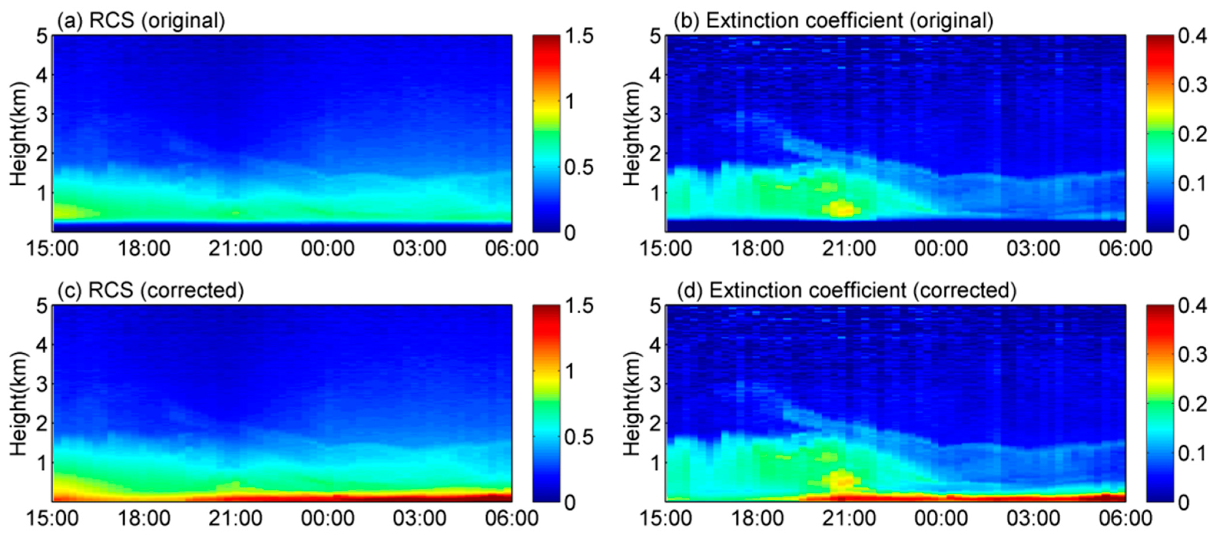
3. Results and Analysis

In May 2019, we conducted a series of simultaneous observations of Lidar and UAV, and obtained eight sets of experimental data, as shown in Figure 1. Each flight takes more than 20 min to smoothly rise by several hundred meters and approximately 10 min to descend. At the same time, three Lidar signal profiles of 355 nm were averaged for processing, with 9000 laser shots transmitted in total. In Figure 1, the black lines are the aerosol extinction coefficient profiles retrieved by Lidar, and the blue lines are the particulate mass concentration profiles measured by the UAV. Affected by the overlap factor, there is a large difference between them at low altitudes, but above 600 m, when the overlap factor approaches one, the trends of the two kinds of profiles are the same. It should be noted that the output values of the data collected by the PMS A003 miniature light scattering particle detector are named after “PM2.5”, which is obviously not rigorous enough. However, since only the conversion relationship needs to be obtained from the acquired data, the impact of this naming is negligible.

A scatter diagram of PM2.5 and extinction coefficients of the coincident profile fragments above 600 m is presented in Figure 2. The relational expression of the dot trace linear fitting is Y = 0.007056X + 0.011, and the coefficient of determination is R² = 0.988.

Data from two different weather conditions are selected to calculate the overlap factors of the Lidar system. Figure 3a–c shows the analysis process of a set of data on the morning of May 13th, local time (LT). First, the particle concentration profile is converted to the extinction coefficient profile, and the wavelet denoising process is performed [29], as shown by the blue and red lines in Figure 3a. The black line in Figure 3a is the aerosol extinction coefficient measured by Lidar. The results are more consistent at altitudes above 0.5 km, and there is a thin cloud at 0.66–0.94 km. Then, the equivalent range corrected signal is calculated from the smoothed extinction coefficient profile according to Equation (1). The red line in Figure 3b represents the range-corrected signal profile after removing the influence of the overlap factor, and the black line represents the original range-corrected signal measured by the Lidar. After adjusting the scale factor, the black line and the red line are consistent in the upper air part. After normalizing the ratio of the two range corrected profiles in Figure 3b and the upper-air part values, the overlap factor profile is obtained, as shown by the red line in Figure 3c. As a comparison, 10 sets (30,000 laser shots in all) of 355 nm and 387 nm signals measured at 22:00 ~ 23:40 (LT) on May 11 were averaged, and the overlap factor was calculated using the Raman method. The result is shown as the black line in Figure 3c. It should be emphasized that the dramatic changes in the density of particles under the cloud make the overlap factors measured by UAV fluctuate significantly between 0.41 and 0.75 km, but the general trends of the overlap factors measured by the two methods are consistent. Figure 3d–f shows an example under clear and clean weather on the afternoon of May 20 (LT), and the content and legend are the same as those in Figure 3a–c. The results show that the overlap factors calculated by the two methods are basically the same. Due to the slight change in the direction of the emitted laser beam between the two experiments, the overlap factor slightly changes.

Demarcated by the time of transmitter adjustment, the data in Figure 1 are divided into two groups. The first set is five groups of data measured on May 12-13 (LT), and the second set is three groups of data measured on May 20 (LT). Intermittent thin clouds appeared at low altitudes in the first group, and the weather in the second group was fine and clean. Figure 4a shows the overlap factor calculated based on the first set of data. The gray area represents the variation range of the five overlap factor profiles, the boundary is the black dashed lines; the black solid line is the averaged overlap factor, and the red dashed line is the result of the Raman method. For comparison, Figure 4b shows the relative deviation of the results of the two methods. The deviation between the two methods is very small above 0.45 km, and the relative deviation between 0.14 and 0.45 km is less than 6.25%. However, the deviation increases rapidly as the altitude decreases and exceeds 10% below 0.12 km. This is because, at low altitudes close to the height of the detection blind zone, the overlap factor value is too small. Figure 4c,d show the calculation results of the second set of data, and the legend is consistent with Figure 4a,b. As the atmosphere is relatively clean and stable, the fluctuation range of the overlap factor is small. The relative deviation is less than 3.55% above 0.26 km and reaches the maximum value of 10.05% at 0.15 km. Below 50 m close to the blind zone, the absolute value of the relative deviation exceeds 10%.

To verify the correction effect of the calculated overlap factor, the overlap factor in Figure 4c is used for data correction from 15:00 on May 22 to 06:00 on May 23 (LT). The time series of 355 nm range corrected signals before and after overlap factor correction are shown in Figure 5a,c, and the corresponding aerosol extinction coefficients are shown in Figure 5b,d, respectively. After 19:30 on 22 July (LT), the near-surface aerosol extinction coefficients gradually increased after overlap factor correction.

To facilitate analysis, the time curves of 75 m, 150 m, 300 m, and 750 m near the height range affected by the overlap factor were selected and compared with the corrected extinction coefficient with the ground observation curve. As shown in Figure 6, before 20:00 on May 22 (LT), due to the relatively uniform mixing of aerosols in the boundary layer, the aerosol extinction coefficients of all heights have the same changing trend, and the values are relatively close. After that, as the top of the boundary layer descends, aerosols converge toward the near-ground area, the changing trend of extinction coefficients at different heights is no longer consistent, and the numerical gap increases. As the height decreases, the trend of the curve gradually coincides with that of the surface ground. To sum up, the ability of Lidar to effectively detect low-altitude aerosols is greatly improved by the correction of the overlap factor.

4. Conclusions

For an aerosol Lidar system that cannot be observed horizontally and does not have a Raman detection channel, a new method of correcting the geometric factor was proposed. The vertical distribution of particulate matter mass concentration detected by the UAV was used to invert the Lidar signal that was not affected by the overlap factor. The inverted signal was compared with the original signal to obtain the required overlap factor. The overlap factor of the 355 nm channel under different weather conditions was obtained from the simultaneous observation of UAV and Lidar. After comparison with the Raman method, it was found that the overlap factor calculated by this method obtains better numerical results. The Lidar’s ability to detect aerosols at low altitudes is significantly improved after the overlap factor had been corrected. In summary, this method provides a new way of correcting the overlap factor for Lidar operating in different complex environments.

References

1. Rosenfeld, D.; Sherwood, S.; Wood, R.; Donner, L. Climate Effects of Aerosol-Cloud Interactions. Science 2014, 343, 379–380. [Google Scholar] [CrossRef]
2. Li, S.; Wang, T.; Solmon, F.; Zhuang, B.; Wu, H.; Xie, M.; Han, Y.; Wang, X. Impact of aerosols on regional climate in southern and northern China during strong/weak East Asian summer monsoon years. J. Geophys. Res. Atmos. 2016, 121, 4069–4081. [Google Scholar] [CrossRef] [Green Version]
3. Barlow, J.F.; Dunbar, T.M.; Nemitz, E.G.; Wood, C.R.; Gallagher, M.W.; Davies, F.; O’Connor, E.; Harrison, R.M. Boundary layer dynamics over London, UK, as observed using Doppler lidar during REPARTEE-II. Atmos. Chem. Phys. Discuss. 2011, 11, 2111–2125. [Google Scholar] [CrossRef] [Green Version]
4. Burkhardt, U.; Kärcher, B.; Schumann, U. Global Modeling of the Contrail and Contrail Cirrus Climate Impact. Bull. Am. Meteorol. Soc. 2010, 91, 479–484. [Google Scholar] [CrossRef] [Green Version]
5. Hsueh, H.T.; Ko, T.H.; Chou, W.C.; Hung, W.C.; Chu, H. Health risk of aerosols and toxic metals from incense and joss paper burning. Environ. Chem. Lett. 2011, 10, 79–87. [Google Scholar] [CrossRef]
6. Zeng, X.-W.; Vivian, E.; Mohammed, K.A.; Jakhar, S.; Vaughn, M.; Huang, J.; Zelicoff, A.; Xaverius, P.; Bai, Z.; Lin, S.; et al. Long-term ambient air pollution and lung function impairment in Chinese children from a high air pollution range area: The Seven Northeastern Cities (SNEC) study. Atmos. Environ. 2016, 138, 144–151. [Google Scholar] [CrossRef] [Green Version]
7. Shen, X.; Sun, J.; Zhang, X.; Zhang, Y.; Zhang, L.; Che, H.; Ma, Q.; Yu, X.; Yue, Y.; Zhang, Y. Characterization of submicron aerosols and effect on visibility during a severe haze-fog episode in Yangtze River Delta, China. Atmos. Environ. 2015, 120, 307–316. [Google Scholar] [CrossRef] [Green Version]
8. Wang, Y.; Chen, L.; Chen, L.; Wang, X.; Yu, C.; Si, Y.; Zhang, Z. Interference of Heavy Aerosol Loading on the VIIRS Aerosol Optical Depth (AOD) Retrieval Algorithm. Remote Sens. 2017, 9, 397. [Google Scholar] [CrossRef] [Green Version]
9. Cohen, J.B.; Prinn, R.G.; Wang, C. The impact of detailed urban-scale processing on the composition, distribution, and radiative forcing of anthropogenic aerosols. Geophys. Res. Lett. 2011, 38. [Google Scholar] [CrossRef]
10. Yang, Y.; Zheng, Z.; Yim, S.Y.; Roth, M.; Ren, G.; Gao, Z.; Wang, T.; Li, Q.; Shi, C.; Ning, G.; et al. PM 2.5 Pollution Modulates Wintertime Urban Heat Island Intensity in the Beijing-Tianjin-Hebei Megalopolis, China. Geophys. Res. Lett. 2020, 47, e2019GL084288. [Google Scholar] [CrossRef] [Green Version]
11. Hua, Y.; Cheng, Z.; Wang, S.; Jiang, J.; Chen, D.; Cai, S.; Fu, X.; Fu, Q.; Chen, C.; Xu, B.; et al. Characteristics and source apportionment of PM2.5 during a fall heavy haze episode in the Yangtze River Delta of China. Atmos. Environ. 2015, 123, 380–391. [Google Scholar] [CrossRef]
12. Zhao, M.; Xie, C.-B.; Zhong, Z.-Q.; Wang, B.-X.; Wang, Z.-Z.; Dai, P.-D.; Shang, Z.; Tan, M.; Liu, N.; Wang, Y.-J. Development of High Spectral Resolution Lidar System for Measuring Aerosol and Cloud. J. Opt. Soc. Korea 2015, 19, 695–699. [Google Scholar] [CrossRef] [Green Version]
13. Zhang, Z.; Huang, J.; Chen, B.; Yi, Y.; Liu, J.; Bi, J.; Zhou, T.; Huang, Z.; Chen, S. Three-Year Continuous Observation of Pure and Polluted Dust Aerosols Over Northwest China Using the Ground-Based Lidar and Sun Photometer Data. J. Geophys. Res. Atmos. 2019, 124, 1118–1131. [Google Scholar] [CrossRef] [Green Version]
14. Hu, S.; Xu, C.; Ji, Y.; Hu, H. Aerosol microphysical parameters’ vertical profiles measured by a dual Raman-Mie lidar during 2007–2013 at Hefei, China. Appl. Opt. 2019, 58, 1537–1546. [Google Scholar] [CrossRef]
15. Yang, H.; Fang, Z.; Xie, C.; Cohen, J.; Yang, Y.; Wang, B.; Xing, K.; Cao, Y. Two trans-boundary aerosol transport episodes in the western Yangtze River Delta, China: A perspective from ground-based lidar observation. Atmos. Pollut. Res. 2021, 12, 370–380. [Google Scholar] [CrossRef]
16. Halldórsson, T.; Langerholc, J. Geometrical form factors for the lidar function. Appl. Opt. 1978, 17, 240–244. [Google Scholar] [CrossRef] [PubMed]
17. Chen, R.; Jiang, Y.; Wen, L.; Wen, D. Calculation of the overlap factor for scanning LiDAR based on the tridimensional ray-tracing method. Appl. Opt. 2017, 56, 4636–4645. [Google Scholar] [CrossRef]
18. Stelmaszczyk, K.; Dell’Aglio, M.; Chudzyński, S.; Stacewicz, T.; Wöste, L. Analytical function for lidar geometrical compression form-factor calculations. Appl. Opt. 2005, 44, 1323–1331. [Google Scholar] [CrossRef]
19. Sasano, Y.; Shimizu, H.; Takeuchi, N.; Okuda, M. Geometrical form factor in the laser radar equation: An experimental determination. Appl. Opt. 1979, 18, 3908–3910. [Google Scholar] [CrossRef]
20. Wandinger, U.; Ansmann, A. Experimental determination of the lidar overlap profile with Raman lidar. Appl. Opt. 2002, 41, 511–514. [Google Scholar] [CrossRef] [PubMed]
21. Chen, H.; Chen, S.; Zhang, Y.; Chen, H.; Guo, P.; Chen, B. Experimental determination of Raman lidar geometric form factor combining Raman and elastic return. Opt. Commun. 2014, 332, 296–300. [Google Scholar] [CrossRef]
22. Li, J.; Li, C.; Zhao, Y.; Li, J.; Chu, Y. Geometrical constraint experimental determination of Raman lidar overlap profile. Appl. Opt. 2016, 55, 4924–4928. [Google Scholar] [CrossRef] [PubMed]
23. Wang, W.; Gong, W.; Mao, F.; Pan, Z. Physical constraint method to determine optimal overlap factor of Raman lidar. J. Opt. 2017, 47, 83–90. [Google Scholar] [CrossRef]
24. Guerrero-Rascado, J.L.; Costa, M.J.; Bortoli, D.; Silva, A.M.; Lyamani, H.; Alados-Arboledas, L. Infrared lidar overlap function: An experimental determination. Opt. Express 2010, 18, 20350–20369. [Google Scholar] [CrossRef] [PubMed]
25. Wang, Z.; Tao, Z.; Liu, N.; Wu, D.; Xie, C.; Wang, Y. New experimental method for lidar overlap factor using a CCD side-scatter technique. Opt. Lett. 2015, 40, 1749–1752. [Google Scholar] [CrossRef]
26. Fernald, F.G. Analysis of atmospheric lidar observations: Some comments. Appl. Opt. 1984, 23, 652–653. [Google Scholar] [CrossRef]
27. Su, J.; Wu, Y.; McCormick, M.P.; Lei, L.; Lee, R.B. Improved method to retrieve aerosol optical properties from combined elastic backscatter and Raman lidar data. Appl. Phys. A 2013, 116, 61–67. [Google Scholar] [CrossRef]
28. Mueller, D.; Ansmann, A.; Mattis, I.; Tesche, M.; Wandinger, U.; Althausen, D.; Pisani, G. Aerosol-type-dependent lidar ratios observed with Raman lidar. J. Geophys. Res. Atmos. 2007, 112, D16202. [Google Scholar] [CrossRef]
29. Zhou, Z.; Hua, D.; Wang, Y.; Yan, Q.; Li, S.; Li, Y.; Wang, H. Improvement of the signal to noise ratio of Lidar echo signal based on wavelet de-noising technique. Opt. Lasers Eng. 2013, 51, 961–966. [Google Scholar] [CrossRef]
Figure 1. (a–h) Aerosol extinction coefficient profiles measured by Lidar (black lines) and PM2.5 profiles measured by UAV (blue lines) at different times that marked in the upper right corner of each sub-figures.
Applsci 12 00184 g001
Figure 2. Scatter diagram of the extinction coefficient and PM2.5 above 600 m.
Applsci 12 00184 g002
Figure 3. Comparison of the results of calculating geometric factors by the two methods under different weather conditions: (ac) thin cloud weather; (df) sunny and clean weather.
Applsci 12 00184 g003
Figure 4. The overlap factors are calculated by the two methods and their relative deviations in different weather conditions: (ab) thin cloud weather; (cd) clean weather.
Applsci 12 00184 g004
Figure 5. Range corrected signal (a,c) and aerosol extinction coefficient (b,d) from 15:00 on May 22 to 06:00 on May 23 (LT) before and after overlap factor correction.
Applsci 12 00184 g005
Figure 6. The curve of the aerosol extinction coefficient with time for different heights.
Applsci 12 00184 g006