An Orthogonal Wheel Odometer for Positioning in a Relative Coordinate System on a Floating Ground

Abstract

This paper introduces a planar positioning sensing system based on orthogonal wheels and encoders for some surfaces that may float (such as ship decks). The positioning sensing system can obtain the desired position and angle information on any such ground that floats. In view of the current method of using the IMU gyroscope for positioning, the odometer data on these floating grounds are not consistent with the real-time data in the world coordinate system. The system takes advantage of the characteristic of the orthogonal wheel, using four vertical omnidirectional wheels and encoders to position on the floating ground. We design a new structure and obtain the position and angle information of a mobile robot by solving the encoder installed on four sets of omnidirectional wheels. Each orthogonal wheel is provided with a sliding mechanism. This is a good solution to the problem of irregular motion of the system facing the floating grounds. In the experiment, it is found that under the condition that the parameters of the four omnidirectional wheels are obtained by the encoder, the influence of the angle change of the robot in the world coordinate system caused by the flotation of the ground can be ignored, and the position and pose of the robot on the fluctuating ground can be well obtained. Regardless of straight or curved motion, the error can reach the centimeter level. In the mobile floating platform experiment, the maximum error of irregular movement process is 2.43 (±0.075) cm and the RMSE is 1.51 cm.

1. Introduction

Robots have been a hot topic ever since the idea of artificial intelligence was raised. The concept of “robot” was first mentioned in the 1920s by Czech writer Karel Capek in his novel, Rossum’s Universal Robot [1]. Among them, the mobile robot is a kind of early development in the field of robot research. In the early 1960s, research on mobile robots was carried out abroad [2]. As the birthplace of robots [3], the United States first realized the first generation of industrial robots and put them into production, for example, Google’s earliest driverless car [4], Da Vinci’s surgical robot [5], and Atlas [6], which represents the most advanced humanoid robot technology in the world.

With the development of robotic research, many robot-related technologies are mature. However, for mobile robots, there are still several aspects worth studying further: First, the mobile robot full-field positioning system. Based on a certain reference position, the mobile robot can obtain the real-time position and attitude of the robot through the data measured by one or more of its own sensors when considering the changes of the environment where the robot is located [7]. The second is the study of path planning. In the known map environment, the mobile robot can dynamically plan a safe and reliable accurate route to reach the feasible target point according to the requirements. Finally, the motion control of mobile robot is studied. On the premise of feasible path planning for the robot, the control robot can reach the target point automatically and safely [8]. All these aspects enable the robot to complete the task. The positioning system of mobile robots is to determine the real-time pose of robots in the environment, which is the basis for the development and application of mobile robots [9]. For mobile robots, posture recognition is the foundation of path planning and motion control. High-precision sensors are needed to detect the pose of mobile robots. Therefore, how to make mobile robot pose detection in a variety of complex environment has become a problem of concern.

At present, there are some mature methods for the study of plane localization: the global navigation satellite system (GNSS) [10,11] and China’s BeiDou navigation satellite system (BDS) [12], which play a major role in outdoor positioning; the pseudolite indoor positioning [13,14] and the indoor positioning system using the beacon [15,16] and Bluetooth [17]; in order to achieve seamless indoor and outdoor positioning services, Chinese researchers are developing a BDS/GPS indoor positioning pseudo-satellite system; precise positioning technology using real-time kinematics (RTK) [18]; using natural or artificial landmarks for positioning, such as two-dimensional code positioning [19]; signal guidance and positioning based on the sensor signals of visual camera [20], RFID [21], ultrasonic [22] and LiDAR [23]; positioning systems using Wi-Fi [24,25] such as (OS-ELM) [26]; inertial navigation and positioning (MEMS) [27]; odometer positioning [28]; etc.

When the robot is on a floating ground (such as the deck of a ship), these positioning methods may not be as effective in obtaining its own posture. When the robot is on the deck, as the ship floats along with the water, the deck is in an irregular motion in both horizontal and vertical directions. In this case, the accuracy of the robot’s positioning is a challenge. For positioning methods such as GPS, GNSS and BDS, which are mainly used for outdoor positioning, signals are blocked when there are obstacles around [29]. In addition to the positioning method mentioned above, the most commonly used positioning system at present is odometer positioning using gyroscopes and orthogonal wheels; although orthogonal wheels are both adopted, the use of gyroscopes has its own limitations in the face of such floating ground. In the following article, we prove the limitations based on experiments.

To solve this problem, we propose a planar positioning sensing system. Figure 1 shows the physical picture of the positioning system. We design a kind of orthogonal wheel structure, which uses four vertical omnidirectional wheels to position on the floating ground. Each driven wheel is equipped with a magnetically coded sensor. Figure 2a shows the installation of the encoder and omnidirectional wheel. The four omnidirectional wheels placed vertically are provided with a sliding mechanism, as shown in Figure 2b, which can move up and down. The range of up and down movement is 6 cm. Every sliding mechanism supports the amount of ground unevenness at ±3 cm. Springs on both sides always provide downward force to the wheels. When the chassis is mounted above the positioning system, it provides downward load to the positioning system so that the wheels can fully contact the ground. In this way, the influence caused by the ground fluctuation on the angle of the robot in the world coordinate system can be ignored, and the motion parameters of the robot in the relative coordinate system relative to the fluctuating ground can be obtained. Finally, the parameters of the four omnidirectional wheels obtained by the sensor can be solved to obtain the pose.

The organization of this paper is as follows. The first part mainly introduces the structure and calculation method of the planar positioning sensor system. The second part proves the limitations of the gyroscope through experiments and analyzes the experimental data of our design of this positioning system. Finally, the experimental results are analyzed and summarized.

2. Materials and Methods

The positioning system is the basic part of an intelligent mobile robot, and it is also one of the key research directions in the field of mobile robots. The orthogonal positioning sensor system introduced in this paper is designed based on the positioning principle of the orthogonal wheel and magnetic encoder. Due to the sudden acceleration of the driving wheel, such as acceleration and emergency stop, the phenomenon of the wheel slipping increases the error of the sensor data. In order to solve the influence of this error, the positioning system designed in this paper adopts the driven way to obtain the position coordinates and rotation angle of the robot relative to the initial pose. The positioning system consists of orthogonal wheels, magnetic encoders and a main frame. Figure 3 shows a three-dimensional diagram of the system.

An orthogonal wheel adopts two identical omnidirectional wheels fixed on the same mechanism. A single orthogonal omnidirectional wheel is shown in Figure 4. Each wheel stand has two degrees of freedom: one is the movement of the axis of the wheel vertically, and the other is the rotation of the axis around the wheel.

The orthogonal wheels assembly includes a bracket and four omnidirectional wheels. The four orthogonal wheels are fixed on the bracket, and the axes of the four orthogonal wheels are perpendicular to each other. Four orthogonal wheels fixed on the bracket can rotate at the same time to achieve any direction of movement. Each driven wheel group includes a sliding mechanism in addition to a bracket and an orthogonal wheel. By designing the sliding mechanism on the bracket of each orthogonal wheel, it is connected with the driven wheel bracket and the whole frame so that the driven wheel group can keep rolling in contact with the ground when sliding in the vertical direction perpendicular to the orthogonal driven wheel shaft. The sliding mechanism consists of a slider, a slide track and a spring. On the floating plane, four orthogonal wheels interact with each other through vertical sliders and slide up and down according to the conditions of the road so that the wheels can always contact the ground, reducing the possibility of wheel slipping and improving the positioning accuracy of the positioning device. Figure 5 shows the tolerance of the positioning system for floating ground.

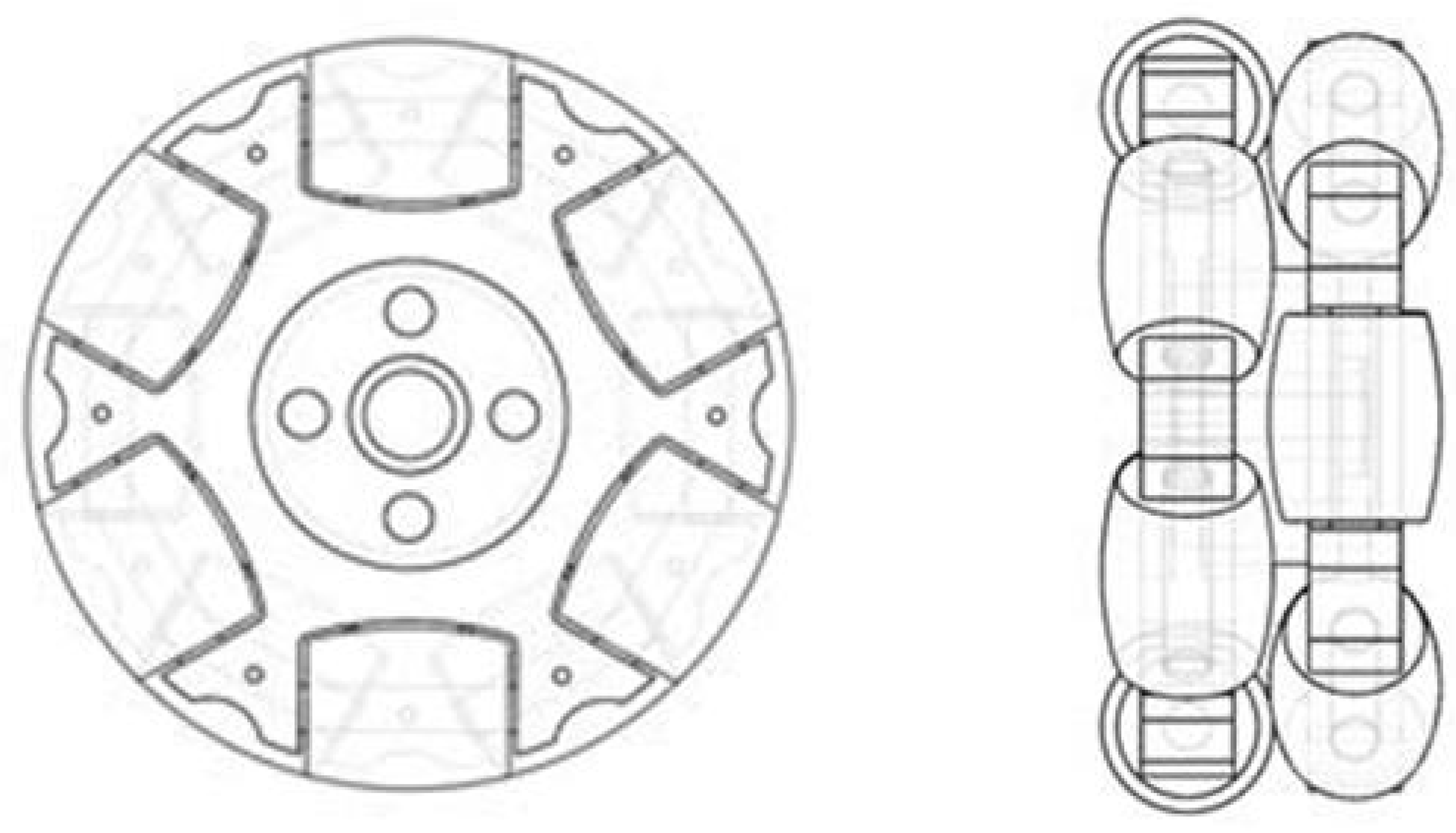
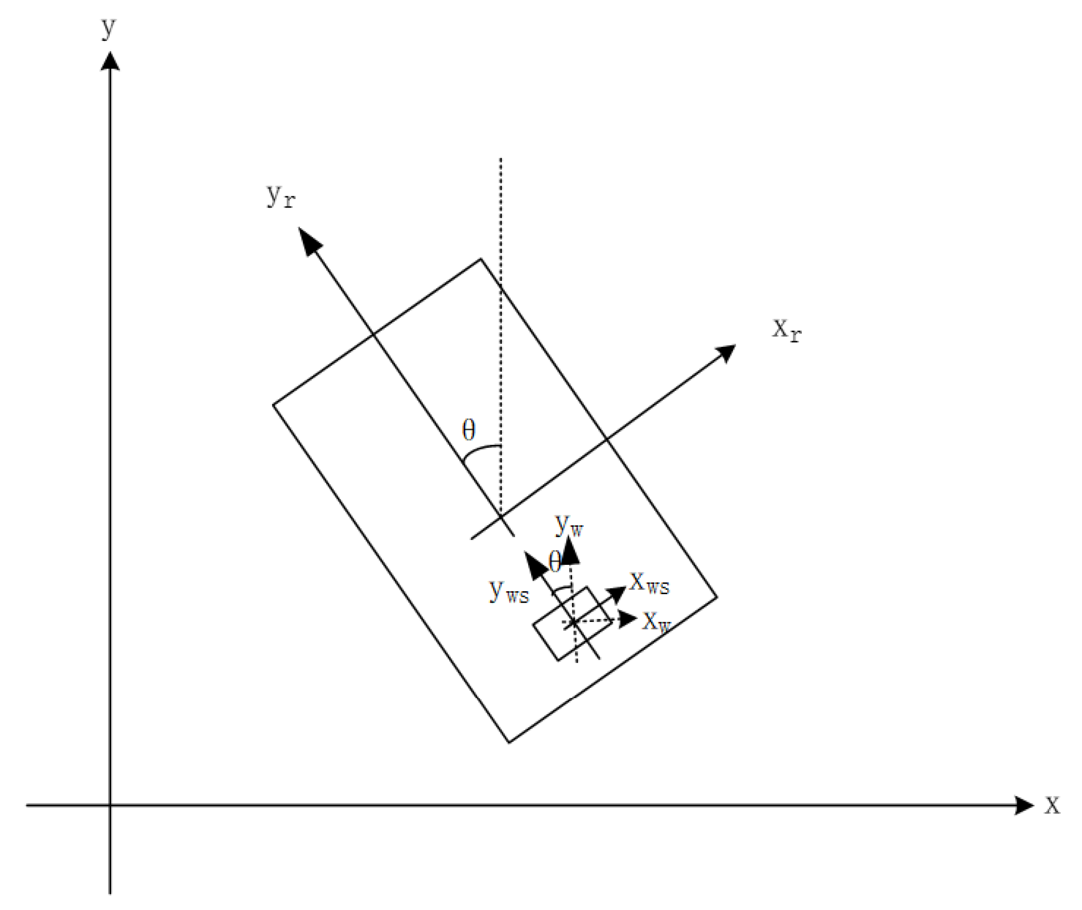
2.1. The Motion Model of a Single Orthogonal Wheel

Counting in the X and Y directions of the orthogonal wheel depends on a magnetic encoder to complete. The dividing value of magnetic encoder is 16,384, that is, one turn corresponds to 16,384. The radius of the orthogonal wheel is 25.4 mm. The displacement of the robot in the X and Y directions can be obtained by integrating the short distance. To determine the real-time accurate pose of the robot in the constructed map, the scheme adopts the relative positioning method. The positioning sensor system is installed on the bottom of the car, and the orthogonal wheels sense the prior position of the robot. For the algorithm of orthogonal wheel odometer, Figure 6 shows the odometer motion model in the X and Y directions of a single orthogonal wheel.

The displacement of the car in the world coordinates and the speed $v_{xws}$ and $v_{yws}$ of the car’s own coordinate system are calculated with the counting of the orthogonal code plate. The coordinate axis X_ws-O-Y_ws shown in the diagram is the coordinate system of the orthogonal wheel group and records the velocity and displacement of the orthogonal wheel group. The angle between the two frames is $\theta$. The distance from the center of the trolley to the installation of the orthogonal wheels is l, and the velocity $v_{xw}$ and $v_{yw}$ of the orthogonal wheel set in the X-O-Y coordinate system is:

$$v_{xw}=v_{xws}cos\left(\theta \right)-v_{y\omega s}sin\left(\theta \right)$$

(1)

$$v_{yw}=v_{yws}cos\left(\theta \right)-v_{x\omega s}sin\left(\theta \right)$$

(2)

The displacement $s_{xw}$ and $s_{yw}$ of the orthogonal wheels in the X-O-Y coordinate system can be calculated by (1) and (2):

$$s_{xw}=\int v_{xw}\mathrm{d}t$$

(3)

$$s_{yw}=\int v_{yw}\mathrm{d}t$$

(4)

Through (3) and (4), the displacement $s_{xr}$ and $s_{yr}$ of the trolley in the X-O-Y coordinate system can be calculated:

$$s_{xr}=s_{xw}+lcos\left(\theta \right)$$

(5)

$$s_{yr}=s_{yw}+lsin\left(\theta \right)$$

(6)

By differentiating both sides of (5) and (6), the velocity $v_{xr}$ and $v_{yr}$ of the car in the X-O-Y coordinate system can be calculated, where $\omega$ is the angular velocity of the car:

$$v_{xr}=v_{xw}-\omega lsin\left(\theta \right)$$

(7)

$$v_{yr}=v_{yw}+\omega lcos\left(\theta \right)$$

(8)

Through (7) and (8), the velocity $v_{xrs}$ and $v_{yrs}$ of the car in the coordinate system of the car itself can be obtained:

$$v_{xrs}=v_{xr}cos\left(\theta \right)+v_{yr}sin\left(\theta \right)$$

(9)

$$v_{yrs}=v_{yr}cos\left(\theta \right)-v_{xr}sin\left(\theta \right)$$

(10)

From the above, the data received through the magnetic encoders on the orthogonal wheels can be converted into the position and velocity information in the world coordinate system. In other words, the velocity and the displacement of the moving chassis in the X-O-Y coordinate system are obtained.

In a simpler sense, the use of two vertically positioned omni-wheels and encoders results in accurate coordinate information relative to the world’s coordinate system, rather than four. In this case, the angle information of the robot can be obtained by using a gyroscope. However, the disadvantages of such positioning systems can be shown when gyroscopes are exposed to floating ground. In subsequent chapters, we prove the defect through experiment.

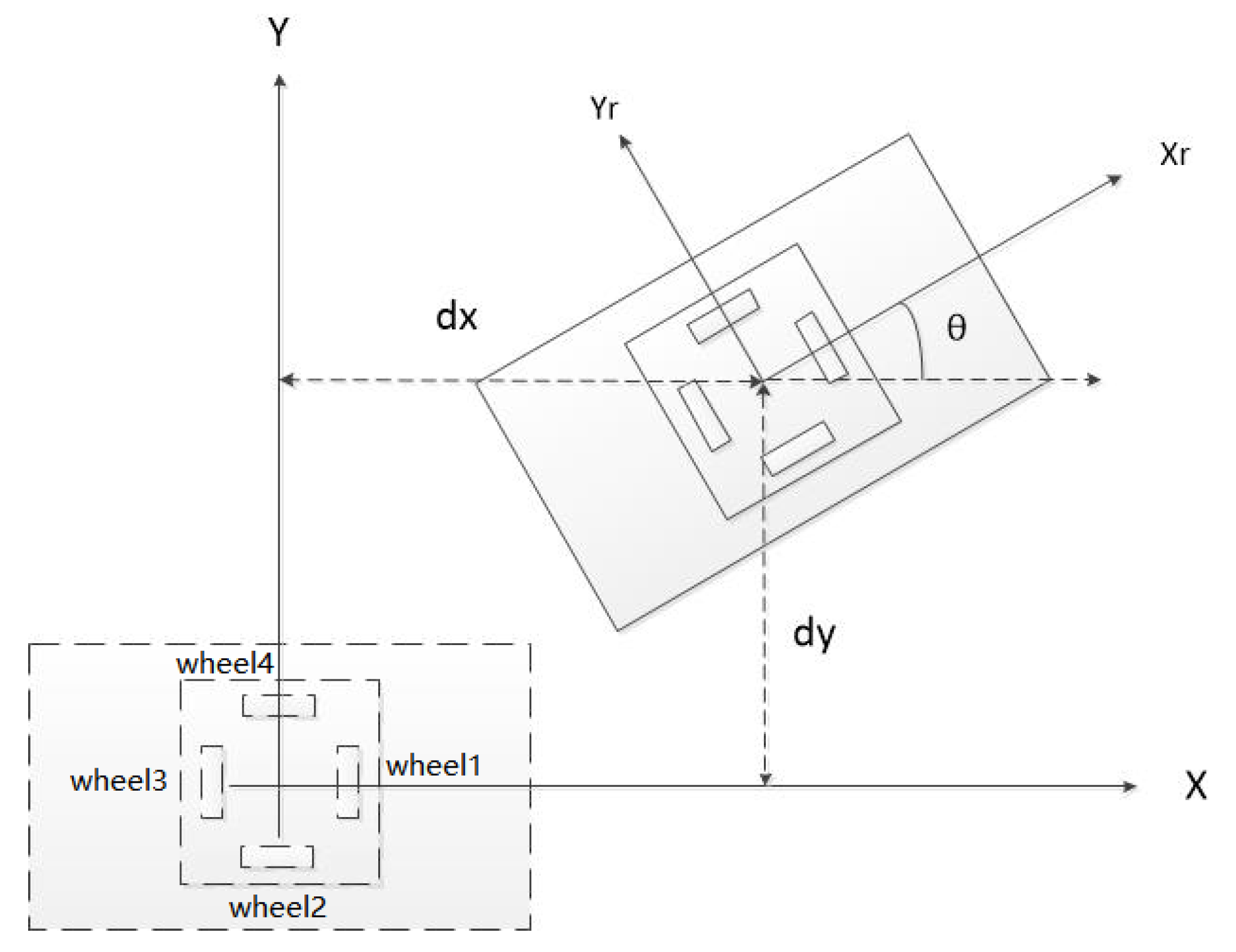
2.2. The Motion Model of Four Orthogonal Wheels

Based on a single wheel, the positioning system we designed uses four orthogonal wheels to solve and obtain accurate coordinate information and angle information. Figure 7 shows the odometer motion model in the X and Y directions of four orthogonal wheels.

Through the linear velocity acquisition module–magnetic encoder, we can obtain the rotation angle ${\theta }_1$, ${\theta }_2$, ${\theta }_3$ and ${\theta }_4$ of each omnidirection from the driving wheel. Given that the radius of each omnidirectional driven wheel is R, the distance $l_1$, $l_2$, $l_3$, $l_4$ of the omnidirectional driven wheel can be calculated. The wheel in the front direction is 1, and clockwise is 2, 3, and 4, as shown in Figure 7:

The wheel axes of the adjacent omnidirectional driven wheels are perpendicular to each other. Through (11), the rotation angle $\theta$ of the mobile robot relative to itself can be calculated:

$$l_n={\theta }_{n}R(n=1,2,3,4)$$

(11)

$$\theta =\frac{l_1+l_2-l_3-l_4}{4L}$$

(12)

By differentiating Equations (11) and (12), we can obtain the distance ${\mathrm{d}}_{l_1}$, ${\mathrm{d}}_{l_2}$, ${\mathrm{d}}_{l_3}$ and ${\mathrm{d}}_{l_4}$ of the omnidirectional rotation from the driving wheel under each instantaneous moment. Then, the displacement dX and dY of the mobile robot in the direction of OX and OY relative to the coordinate system XOY with itself as the origin is obtained at every instantaneous moment:

$$\mathrm{d}\mathrm{X}=\frac{{\mathrm{d}}_{l_2}-{\mathrm{d}}_{l_4}}{2}cos\left(\theta \right)-\frac{{\mathrm{d}}_{l_1}-{\mathrm{d}}_{l_3}}{2}sin\left(\theta \right)$$

(13)

$$\mathrm{d}\mathrm{Y}=\frac{{\mathrm{d}}_{l_1}-{\mathrm{d}}_{l_3}}{2}cos\left(\theta \right)-\frac{{\mathrm{d}}_{l_2}-{\mathrm{d}}_{l_4}}{2}sin\left(\theta \right)$$

(14)

By integrating the displacement dX and dY in the direction of OX and OY at every instantaneous moment, the displacement $\Delta$X and $\Delta$Y in the direction of OX and OY relative to the origin position of the mobile robot can be obtained:

$$\Delta \mathrm{X}=\int \mathrm{d}\mathrm{X}\mathrm{d}t$$

(15)

$$\Delta \mathrm{Y}=\int \mathrm{d}\mathrm{Y}\mathrm{d}t$$

(16)

Thus, the data received by the magnetic encoders on the orthogonal wheels can be converted into position and velocity information in the world coordinate system. That is, the displacement of $\Delta$X and $\Delta$Y relative to the origin position of the mobile robot and the rotation angle relative to itself are obtained.

In the next chapter, the positioning module using an orthogonal wheel and gyroscope is compared with the positioning sensor system we designed to illustrate the disadvantages of using a gyroscope in some specific situations and the advantages of the positioning sensor system introduced in this paper. The positioning sensor system mainly collects and processes the encoder data on the orthogonal wheels to calculate the real-time position and pose state of the positioning system. Through the acquisition of encoder data, the data are transferred to the central processing unit, and then the central processing unit calculates the pose state of the mobile robot and transmits it to the upper computer through the serial port.

3. Experiments

Figure 8 shows the system flow chart of the positioning system we designed. The positioning system using gyroscope mainly collects and processes the data of gyroscope and encoder, and then transfers it to the central processing unit for processing and uploading to the upper computer. Figure 9 shows a system flow chart for a positioning system using a gyroscope.

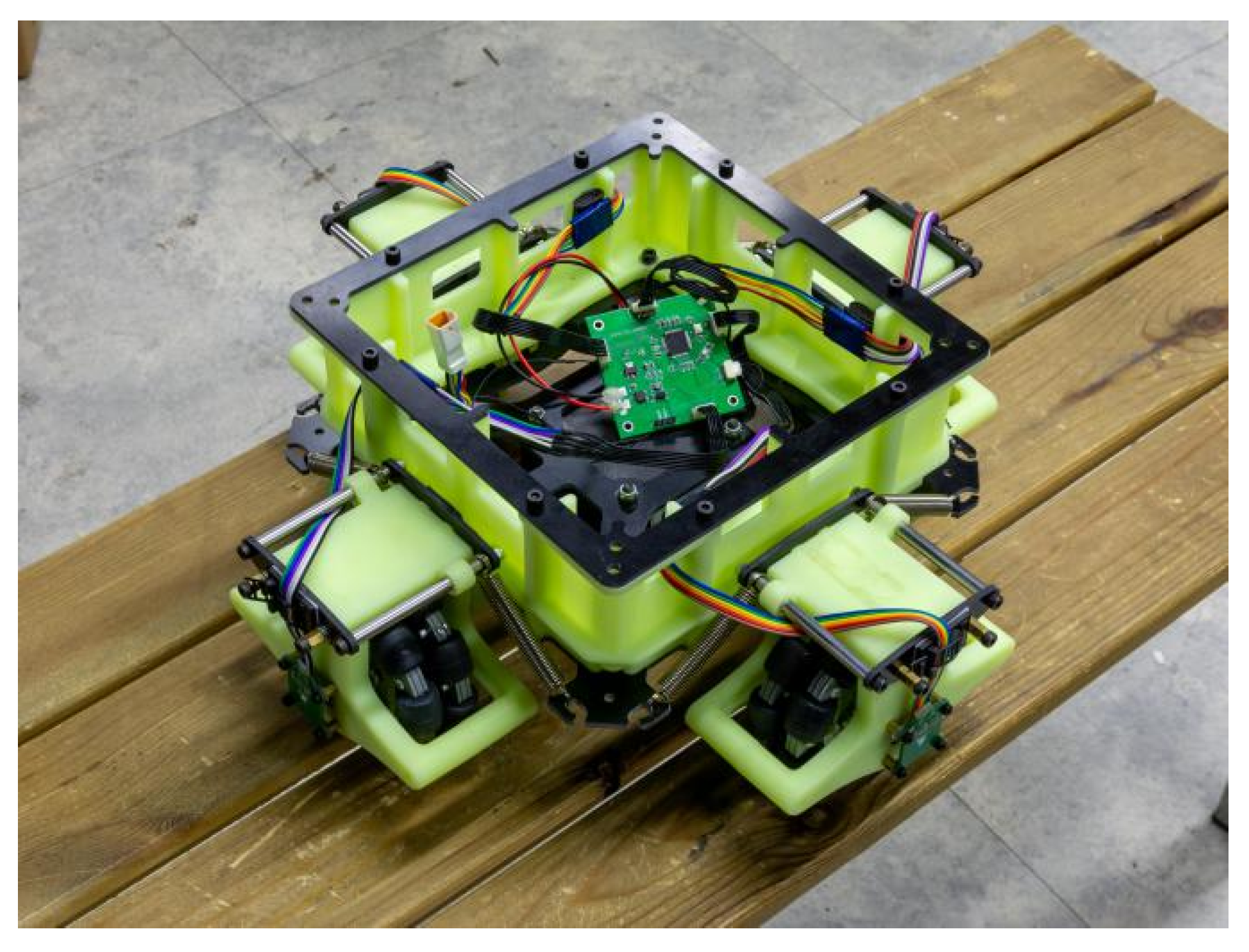
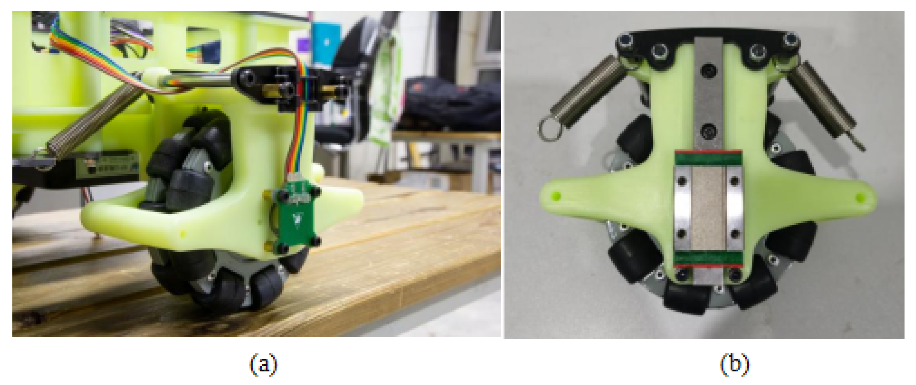
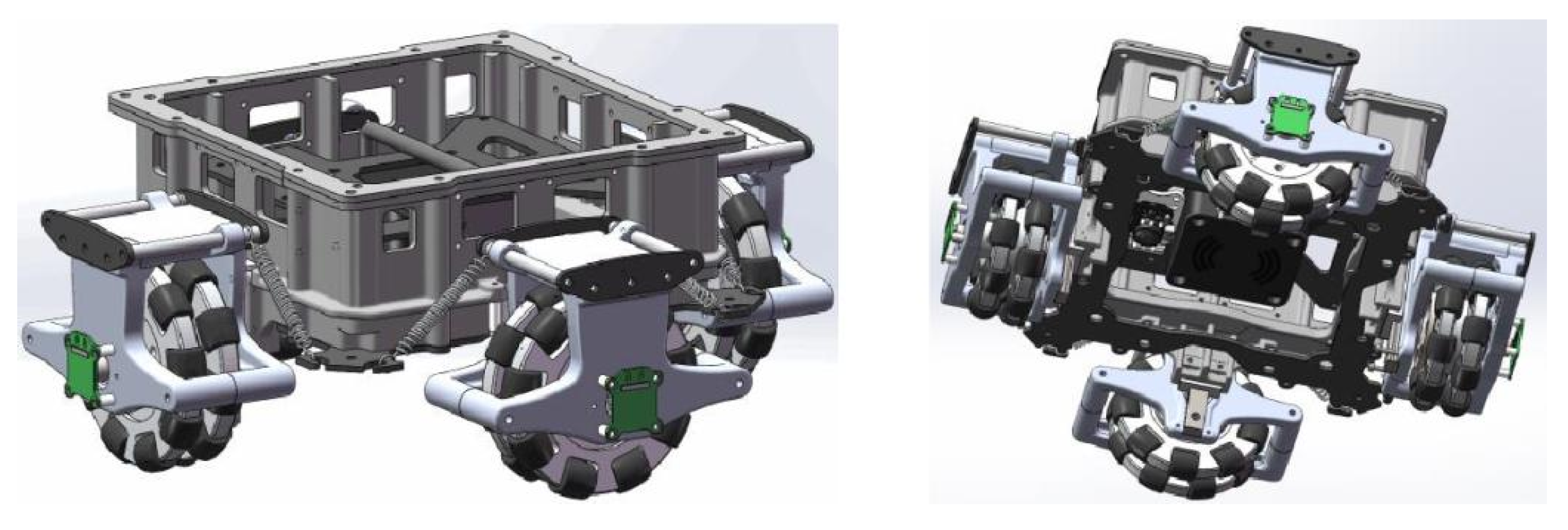
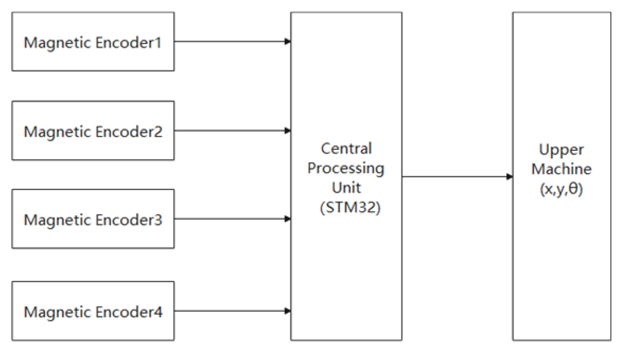
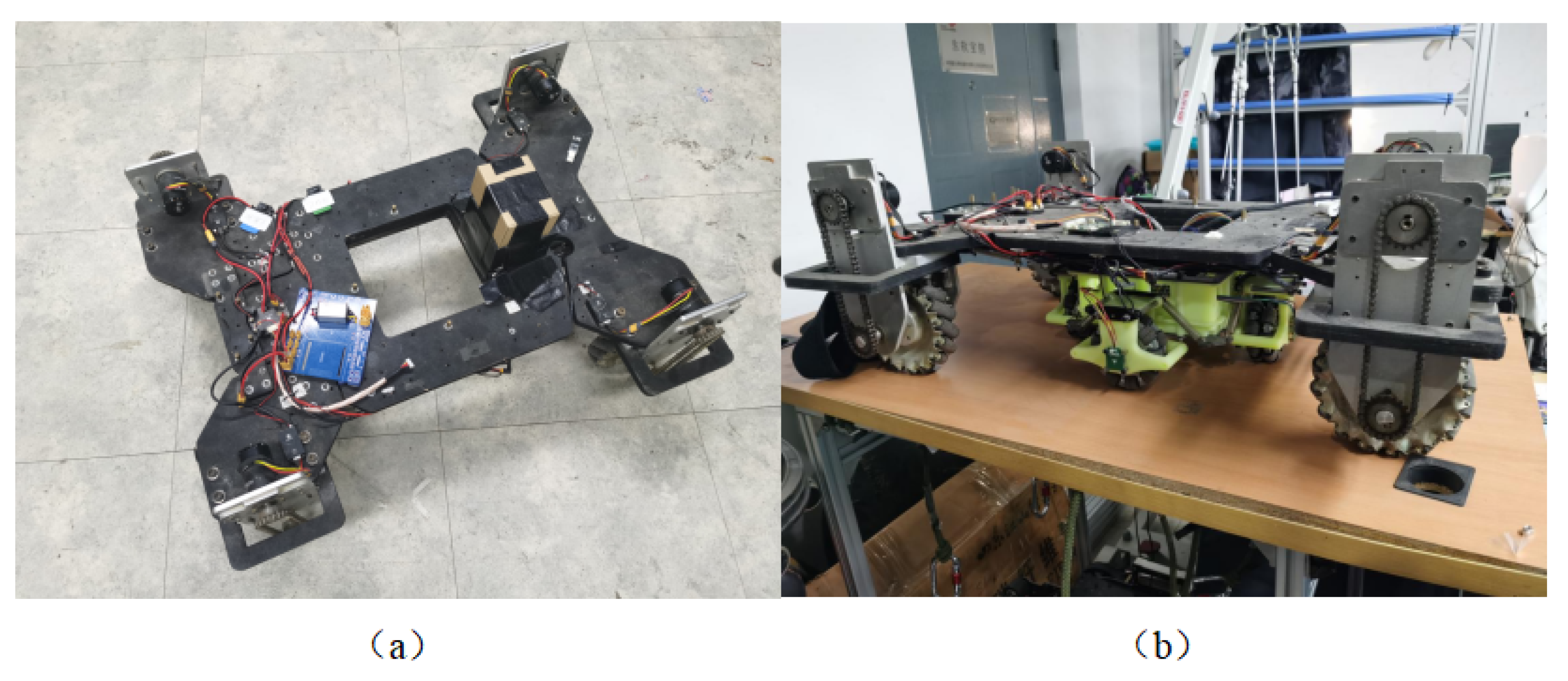
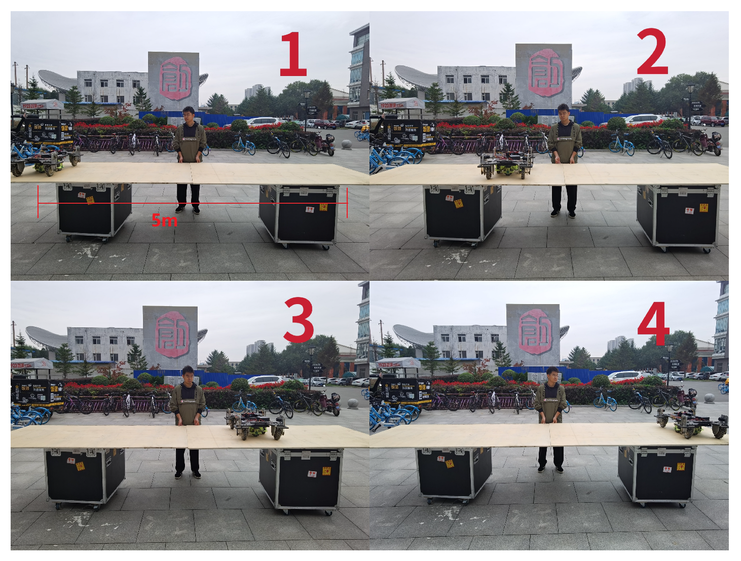
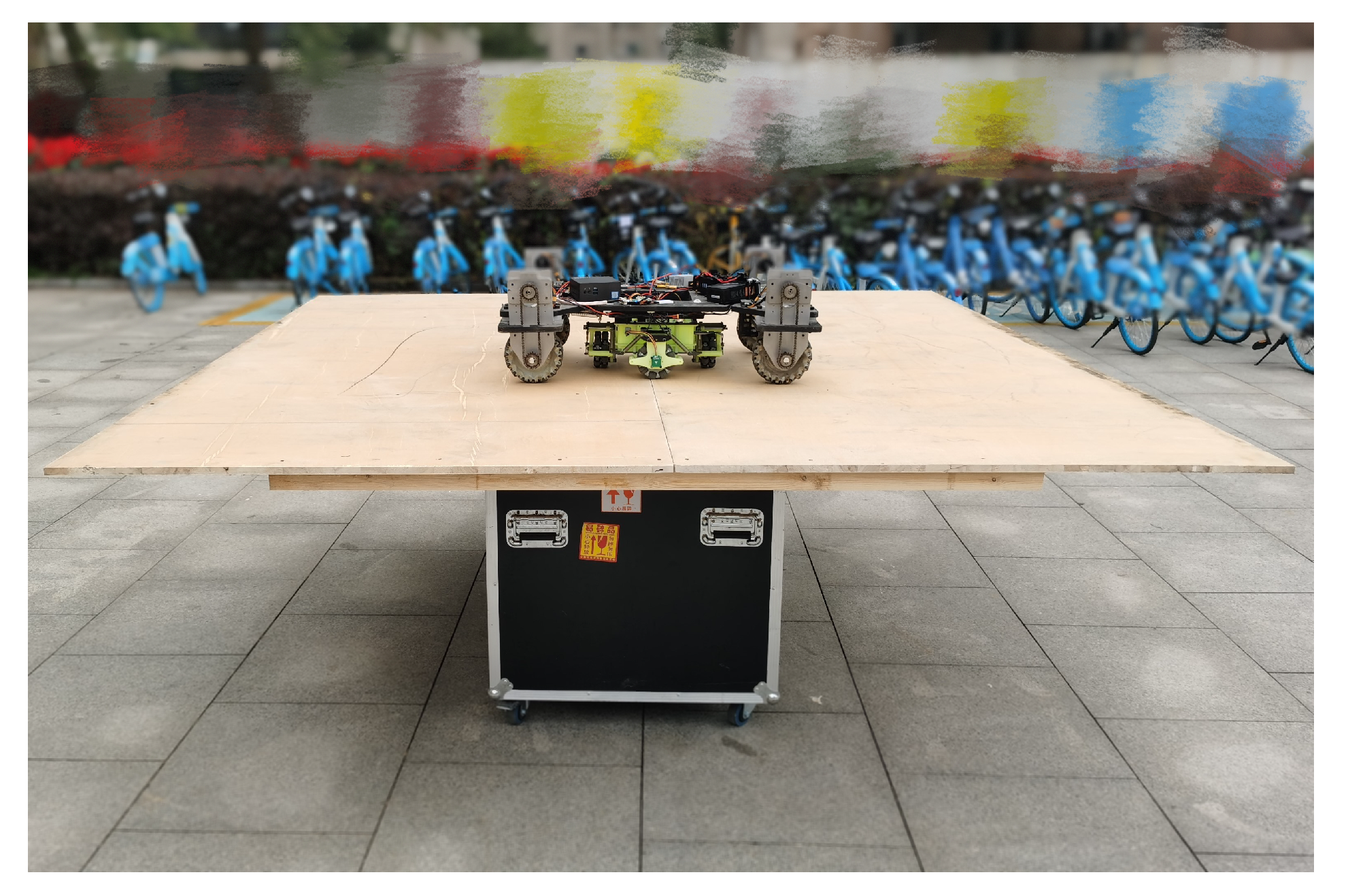
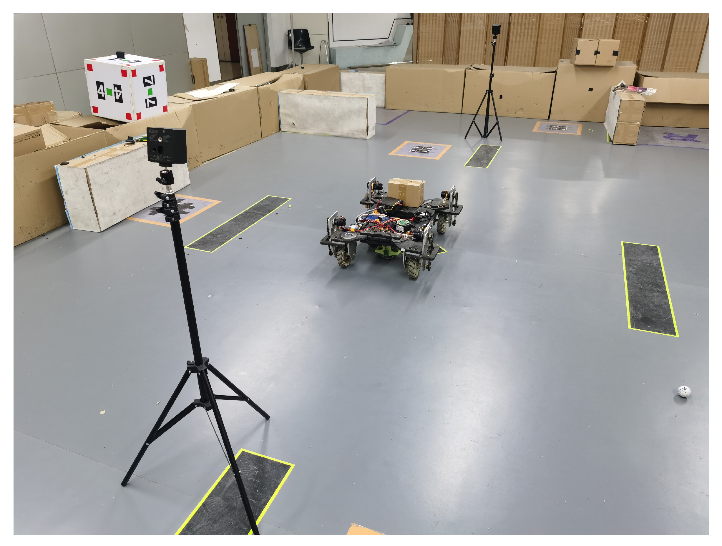
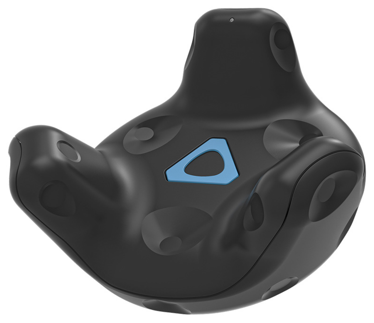
3.1. The Experiment Equipment

This section discusses the positioning device developed on the mobile robot chassis platform. Figure 10 shows the chassis platform of the mobile robot in this experiment. The data collected by the chassis platform are used to analyze the positioning effect. The experiment involves linear motion, curved motion, and rotation around the center of the robot. The positioning system transmits the output position information to the upper computer and draws the time displacement curve of the mobile robot.

Figure 11 shows the chassis coordinate diagram of mobile robot.

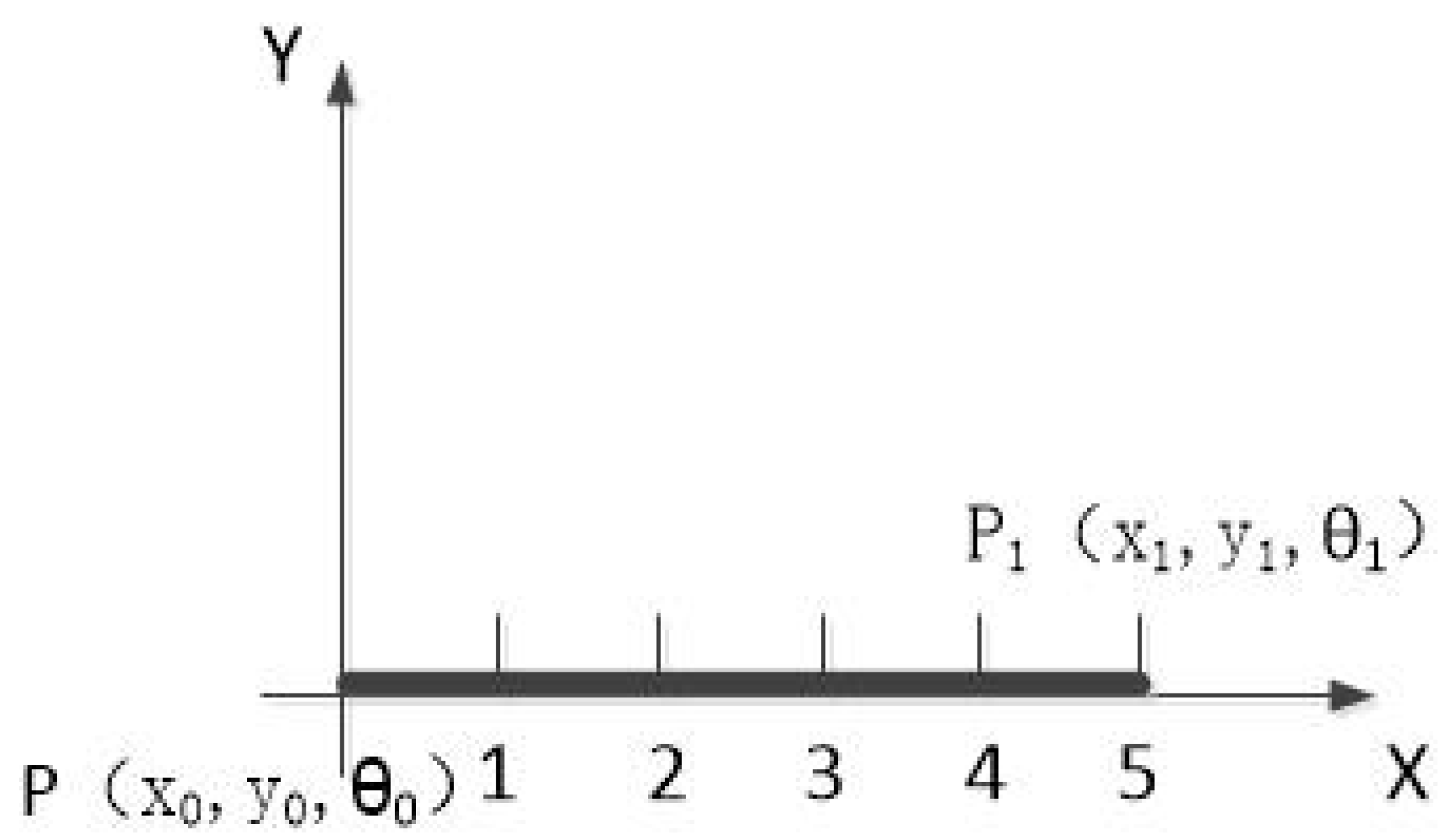
3.2. The Experiment of Linear Motion

In order to simulate the floating ground, we built a floating platform with a size of 5.4 m × 1.3 m, as shown in Figure 12. During the movement of the moving chassis, the platform is disturbed by the irregular up and down movement, artificially. The platform floats mainly by artificial up and down motion. The floating platform can have six degrees of freedom because it has multiple universal wheels under it. The wheels under the platform are locked, and the platform is only artificially pitched and rolled. In addition, the floating degree of platform can be obtained by installing IMU on the moving chassis. Through IMU and the position system, the six degrees of freedom of moving chassis can be obtained, so the floating degree of the simulated platform can be reflected by the angle of chassis coiling around the pitch and roll axis. For pitch and roll angles, we mainly limit them to 15°.

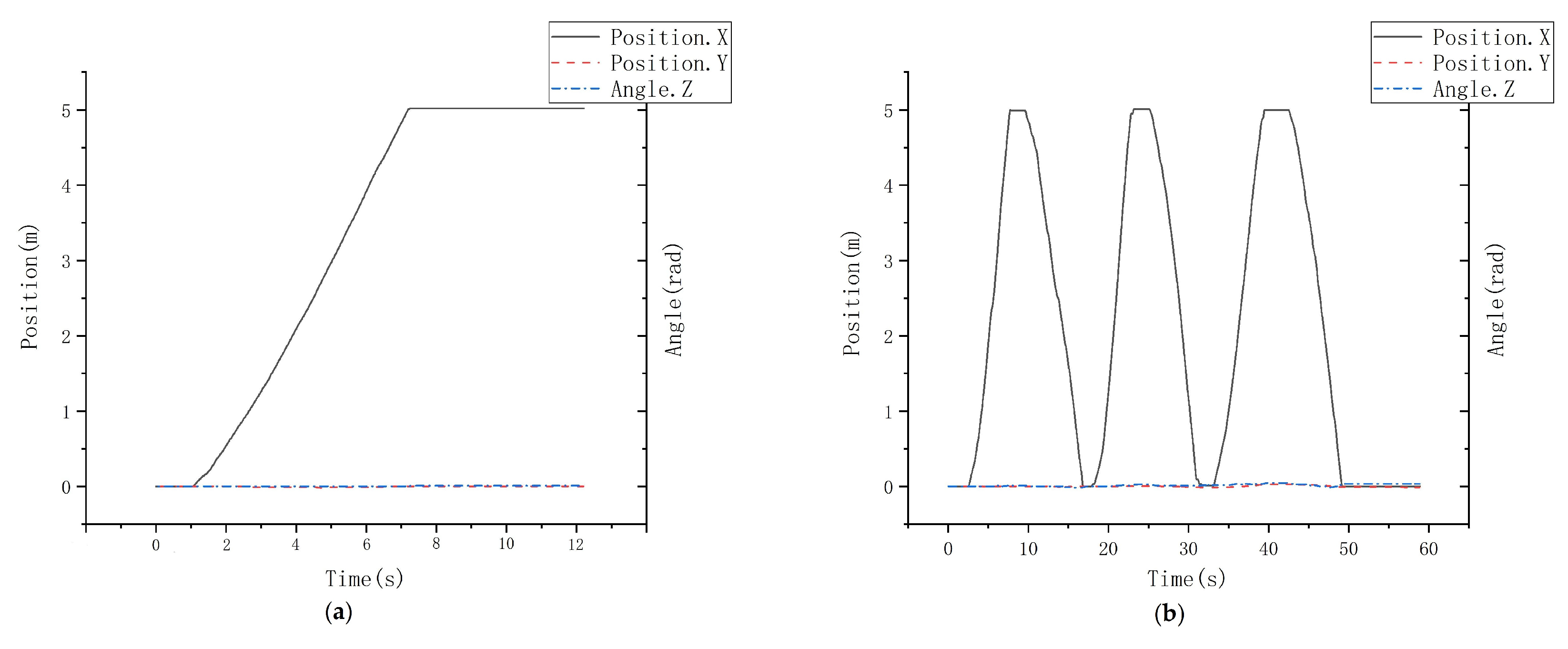
3.2.1. The Chassis Moves in the X Direction

In the initial case, the front of the chassis is oriented in the positive direction of the X axis. The chassis moves in the X direction from point P to point ${\mathrm{P}}_1$ with a motion distance of 5 m. Figure 13 shows the movement track of the moving chassis. During the movement, the floating platform is artificially disturbed by moving up and down. The actual motion scene in the X direction is shown in the Figure 14.

The travel displacement transformation curve of the mobile robot chassis is shown in Figure 15. In the process of motion, due to the linear motion along the X axis, the displacement of the Y axis and the angle of the Z axis basically do not fluctuate. The floating degree of the simulated platform can be reflected by the angle of chassis coiling around pitch and roll axis, as shown in Figure 16.

Table 1. The actual movement value and error of the positioning system for each movement of 5 m along the X axis.

The Theoretical Movement Value (cm)	The Actual Movement Value (cm)	Error (cm)
500	500.5	0.5
500	500.3	0.3
500	500.8	0.8
500	501.1	1.1

records the actual movement value and error of the positioning system for each movement of 5 m along the X axis. It can be seen from Table 1 the positioning value after each movement of 5 m. In addition, the cumulative error of the positioning system is approximately 1.1 cm after it moves a distance of 5 m continuously for four times in the X direction. The experiment shows that the positioning system can meet the requirements in the short distance.

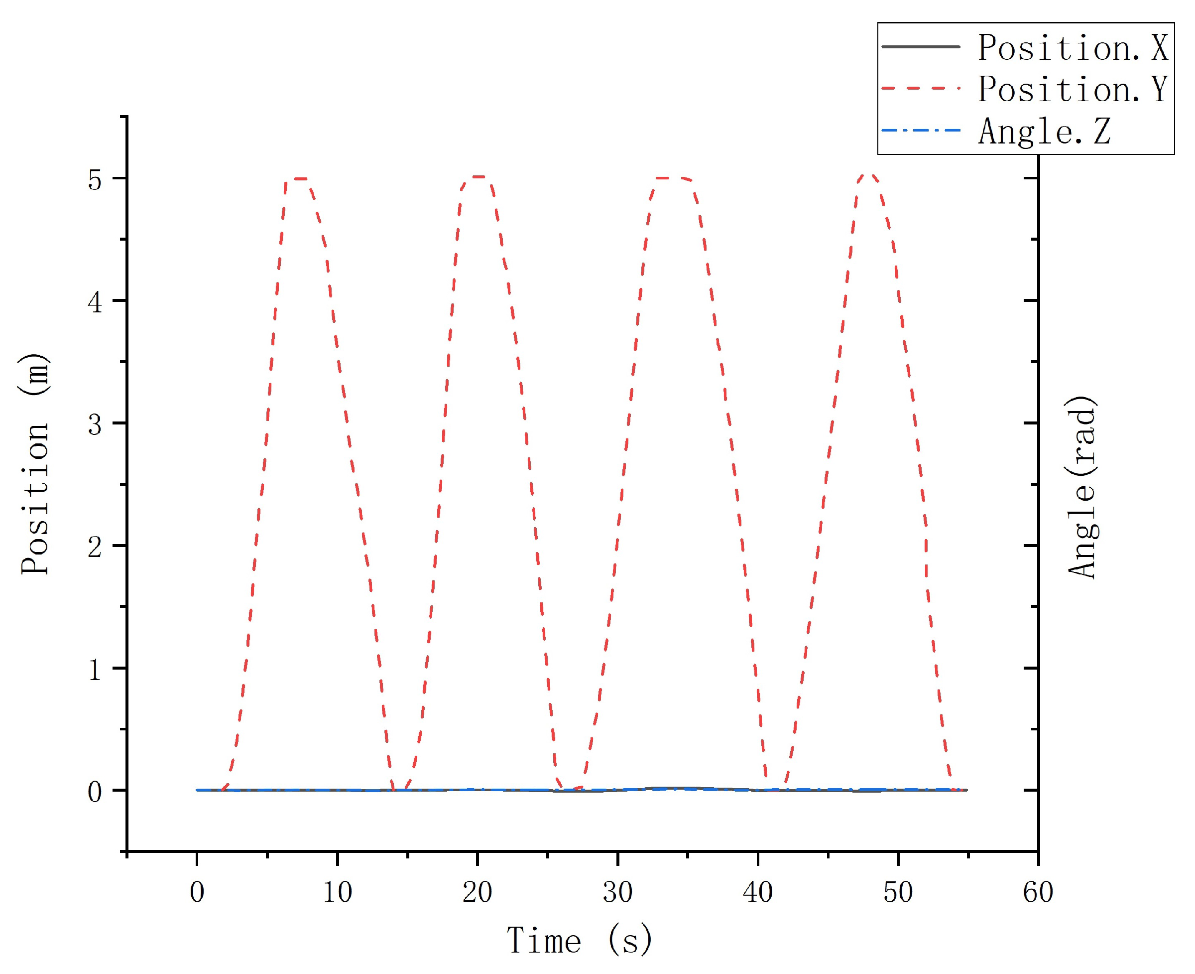
3.2.2. The Chassis Moves in the Y Direction

The moving chassis uses the Mecanum wheel, which provides freedom of movement in the Y direction. Therefore, this chassis can be used to detect the positioning error of our self-developed positioning system in the Y direction. The actual motion scene in the X direction is shown in the Figure 17.

The travel displacement transformation curve of the mobile robot chassis is shown in Figure 18. In the process of motion, due to the linear motion along the Y axis, the displacement of the X axis and the angle of the Z axis basically do not fluctuate. Figure 19 shows that the angle of chassis coiling around pitch and roll axis.

Table 2. The actual movement value and error of the positioning system for each movement of 5 m along the Y axis.

The Theoretical Movement Value (cm)	The Actual Movement Value (cm)	Error (cm)
500	500.1	0.1
500	500.3	0.3
500	500.7	0.7
500	501.0	1.0

records the actual movement value and error of the positioning system for each movement of 5 m along the Y axis. It can be seen from Table 2 the positioning value after each movement of 5 m. In addition, the cumulative error of the positioning system is approximately 1.0 cm after it moves a distance of 5 m continuously for four times in the Y direction. The experiment shows that the positioning system can meet the requirements in the short distance.

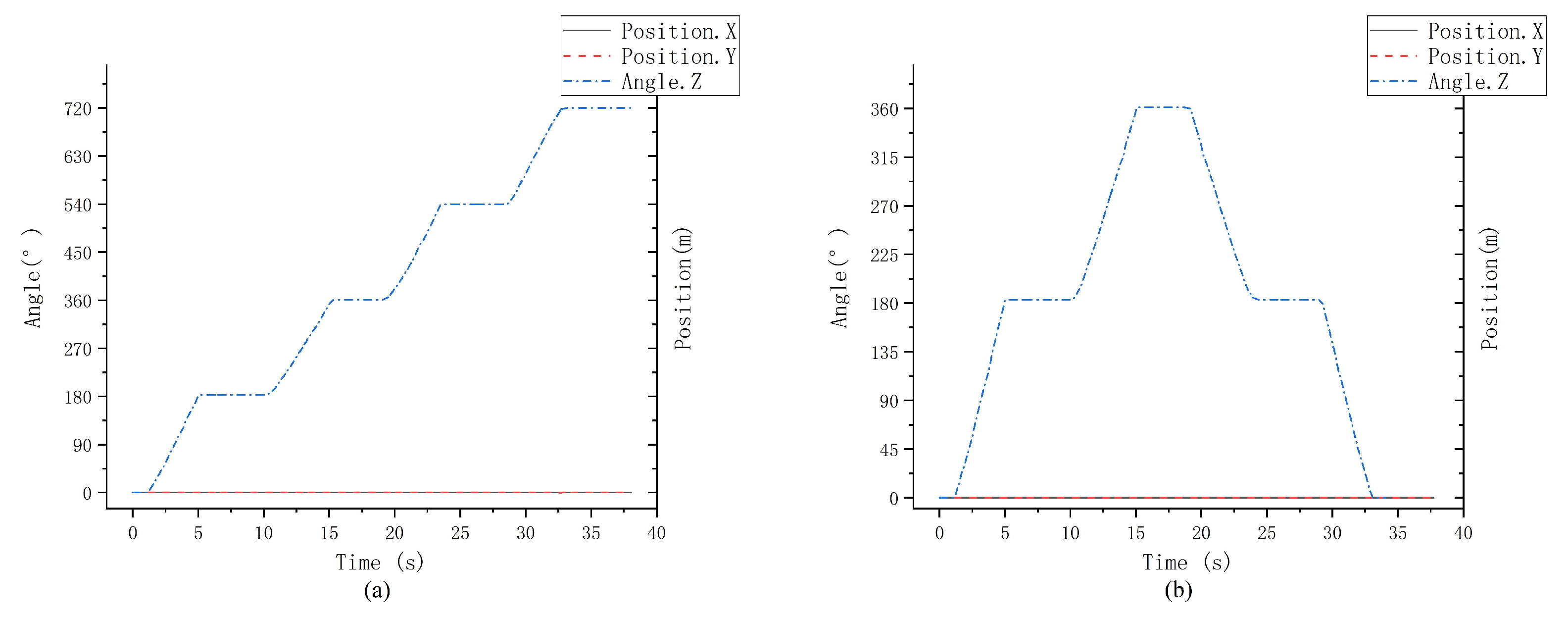
3.2.3. The Experiment of Rotational Motion

In order to verify the accuracy of the angle of the orthogonal wheel positioning system, the chassis of the mobile robot rotates around the center of the body and stops once every 180° for two consecutive turns. The actual motion scene of the chassis rotation is shown in the Figure 20. Figure 21 shows the angle curve of the moving chassis as it rotates in situ. During the rotation of the moving chassis, the displacement along the X and Y directions appears very small fluctuations because the center of the chassis and the center of the orthogonal wheels do not coincide completely. Figure 22 shows that the angle of chassis coiling around pitch and roll axis.

Table 3. The actual movement value and error of the positioning system for each movement of 180° along the Z axis.

The Theoretical Angle Value (°)	The Actual Angle Value (°)	Error (°)
180.00	180.12	0.12
360.00	360.42	0.42
540.00	540.62	0.62
720.00	721.15	1.15

shows the actual angle value and error of the positioning system for each rotation of 180° around the Z axis. Table 3 shows the positioning values after each rotation of 180°. In addition, the cumulative error of the positioning system is approximately 1.15° after continuous rotation of 720° around the Z axis. The experiment shows that the precision of rotation angle of the positioning system is satisfactory.

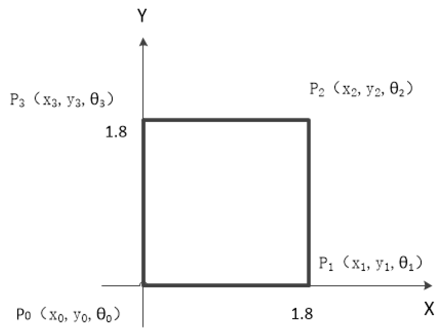
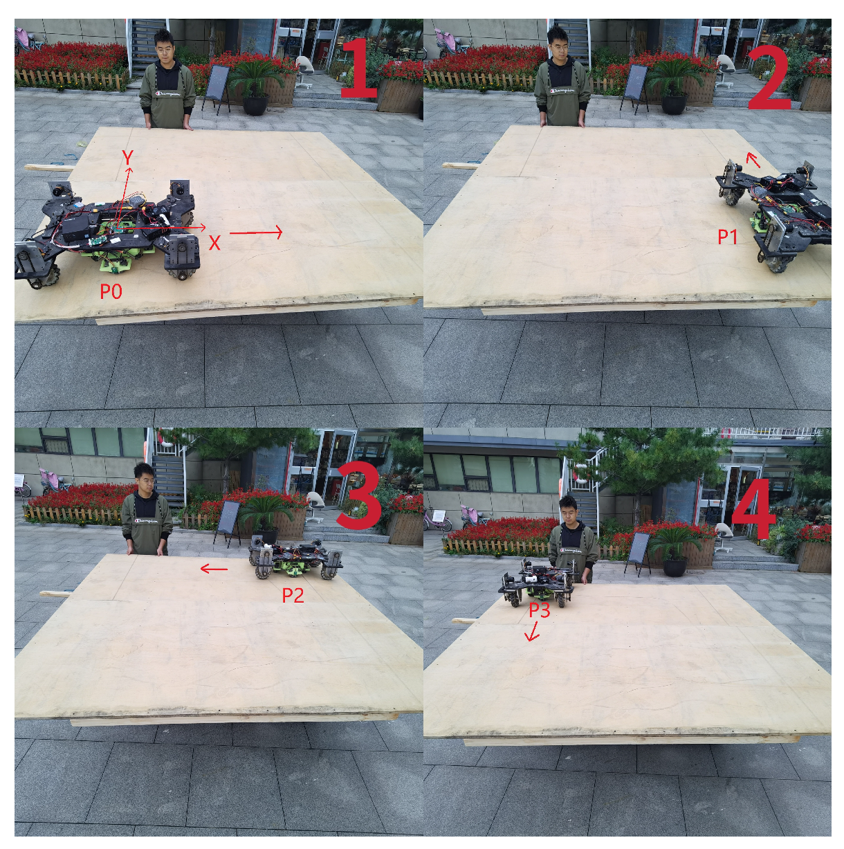
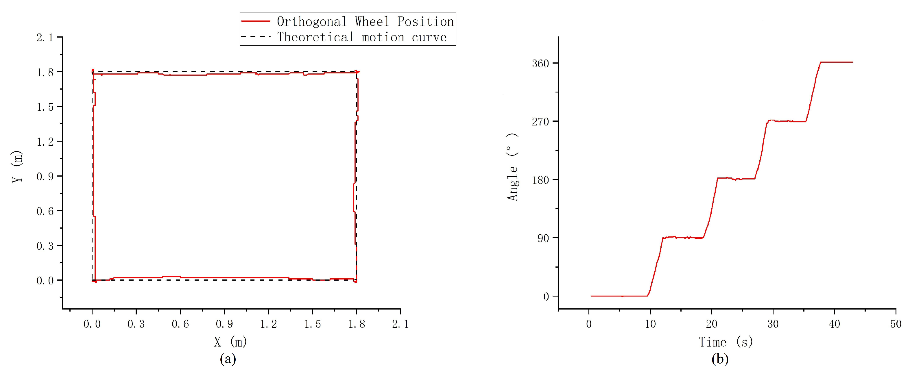
3.2.4. The Experiment of Moving along a Square

The mobile robot chassis moves in a square counterclockwise direction along the simulated floating platform as shown in Figure 23.

Due to the size limitation of the floating platform, we choose the side length of the square to be 1.8 m. Figure 24 shows the movement track of the mobile chassis. The positioning effect of the positioning module is verified by the movement of the chassis along the square. The four points of the square are set to ${\mathrm{P}}_0$, ${\mathrm{P}}_1$, ${\mathrm{P}}_2$, and ${\mathrm{P}}_3$. The actual motion scene is shown in Figure 25.

The displacement transformation curve and angle change curve of the mobile robot chassis are shown in Figure 26. In the process of movement, the actual motion curve is basically consistent with the theoretical motion curve, with only a little fluctuation. The floating degree of the simulated platform can be reflected by the angle of chassis coiling around pitch and roll axis, as shown in the Figure 27.

Table 4. The actual movement value and error of the positioning system for each point along the square.

	Theoretical Movement Value			Actual Movement Value			Error
	x(m)	y(m)	$\mathit{\theta }$(°)	x(m)	y(m)	$\mathit{\theta }$(°)	$\Delta$d(m)	$\Delta$$\mathit{\theta }$(°)
$P_0$	0	0	0	0	0	0	0	0
$P_1$	1.80	0	90	1.802	−0.008	90.02	0.008	0.02
$P_2$	1.80	1.80	180	1.808	1.795	181.45	0.009	0.45
$P_3$	0	1.80	270	0.011	1.805	270.87	0.012	0.87
$P_0^{\prime }$	0	0	360	0.013	−0.010	361.42	0.016	1.42

records the actual movement value and error of the positioning system for each point along the square. It can be seen from Table 4 the positioning value after moving to each point along the square. In addition, after the positioning system returns to the origin after four points, the distance cumulative error is approximately 1.6 cm, and the angle cumulative error is approximately 1.42°. The experiment shows that the positioning system can meet the requirements in the short distance.

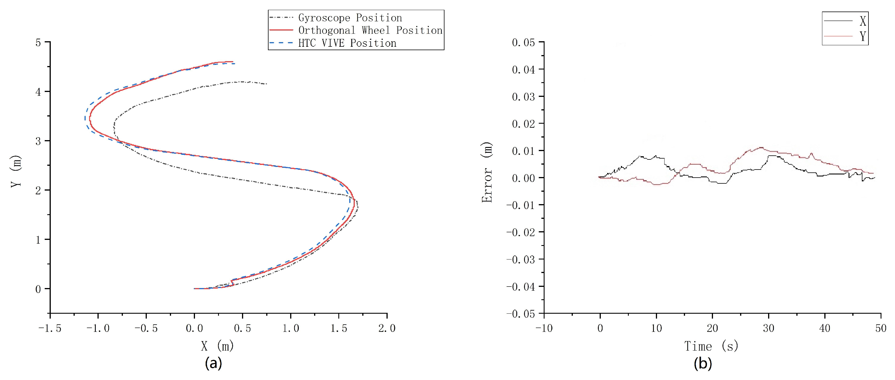
3.3. The Experiment of Random Curve Motion

Before we talk about the experiment, let us first introduce the Steam VR tracking system based on HTC VIVE used in the experiment [30]. This system has long been used in VR motion-sensing games. It is equipped with STEAM tracking technology that allows accurate positioning within a space area of 6 m × 6 m, with an accuracy of less than 1 mm. It includes two HTC VIVE2.0 location base stations and a tracker. By installing the tracking device used in the joystick in the motion sensing game on the chassis of the mobile robot, we can obtain the most accurate actual curve in the random curve movement so as to carry out comparative experiments with the orthogonal wheels positioning system and gyro positioning system designed by us.

First, we introduce the experimental site of random curve motion experiment. Figure 28 shows the site layout of the laboratory. The HTC VIVE2.0 base stations are placed on both sides. The base station is placed on the same axis with a height of one meter. The tracker as shown in Figure 29 is mounted on the mobile chassis, which is fixed in the center of the mobile chassis, that is, the center of the orthogonal wheels system. The mobile robot is randomly moved, S-shaped, by the remote control.

In this experiment, we conducted a comparative experiment on our own positioning system, the gyroscope positioning system and the HTC VIVE positioning system. In the experiment, the gyroscope positioning system can obtain the rotation angle in the movement process by itself, and at the same time, the data of two mutually perpendicular wheels of the four wheels in the orthogonal wheel system serve as the data of X and Y. According to the solution method mentioned in Section 2.1, coordinate information of gyroscope positioning can be obtained. In the process of random S-shaped motion, the upper computer can obtain the data of orthogonal wheel positioning and gyroscope positioning at the same time for comparison test. In combination with the data obtained by HTC VIVE, three experimental curves can be obtained at the same time in one movement for comparison. Figure 30 shows the gyroscope position curve, orthogonal wheels position curve, HTC VIVE position curve and the error curve of orthogonal wheels relative to HTC VIVE, respectively.

As can be seen from the comparison curve, the positioning curve of the orthogonal wheels positioning system is basically consistent with that of HTC VIVE in the random S-shaped motion, and the maximum error is 1.18 (±0.075) cm in the process of moving. As for the positioning curve of the positioning system using a gyroscope, the deviation degree of the curve is increasing with the progress of the motion, due to the accumulated error of gyroscope rotation during the traveling process. This is due to the orthogonal wheel positioning system, which does not have the same sudden or continuous rotation as a gyroscope, resulting in a large deviation in the angle acquisition.

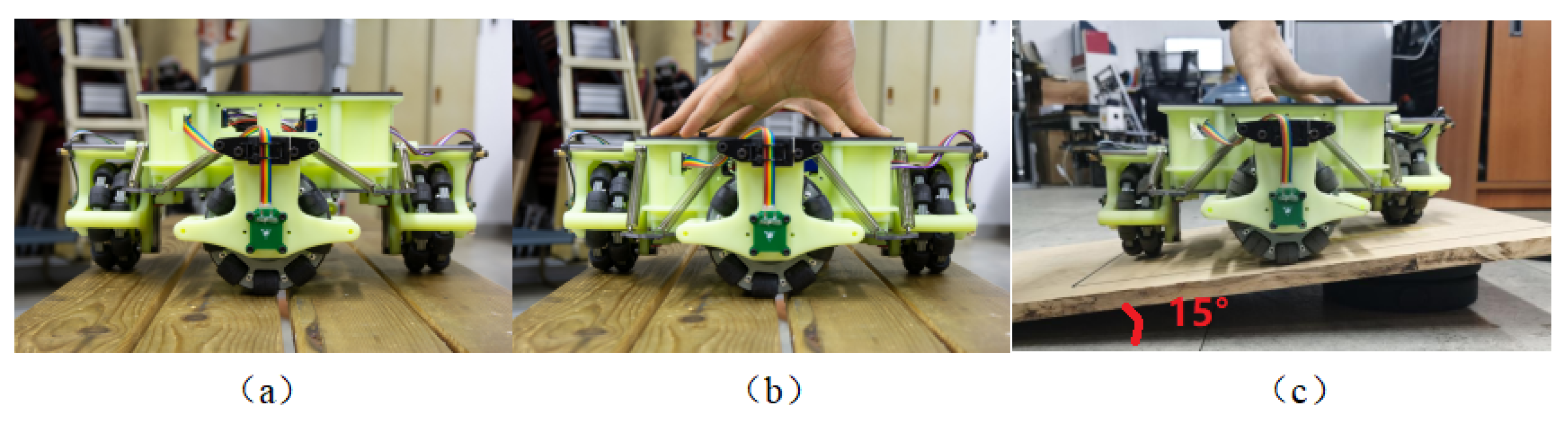
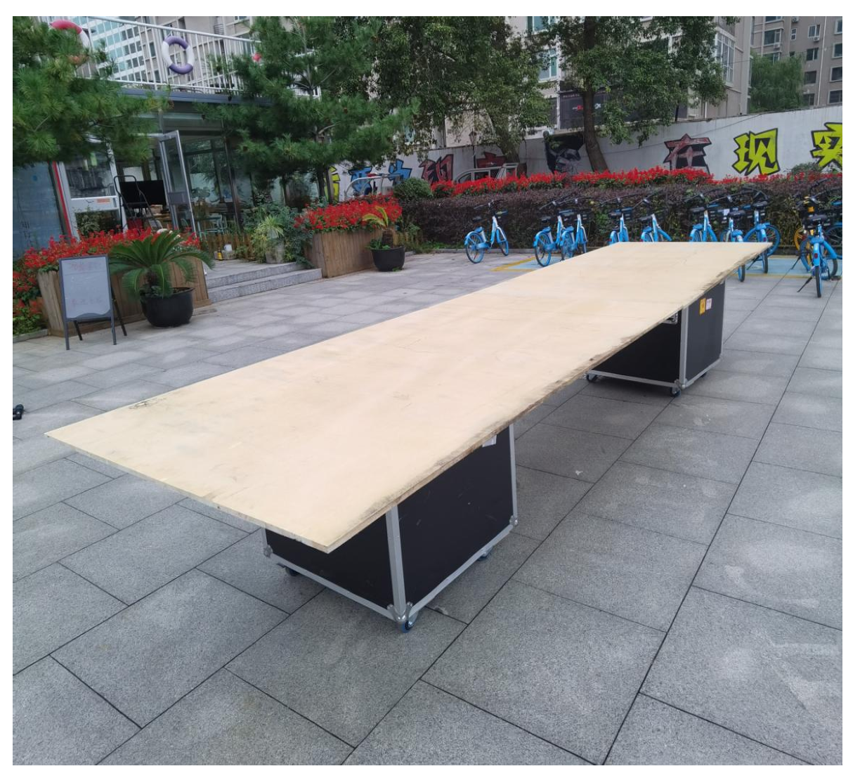
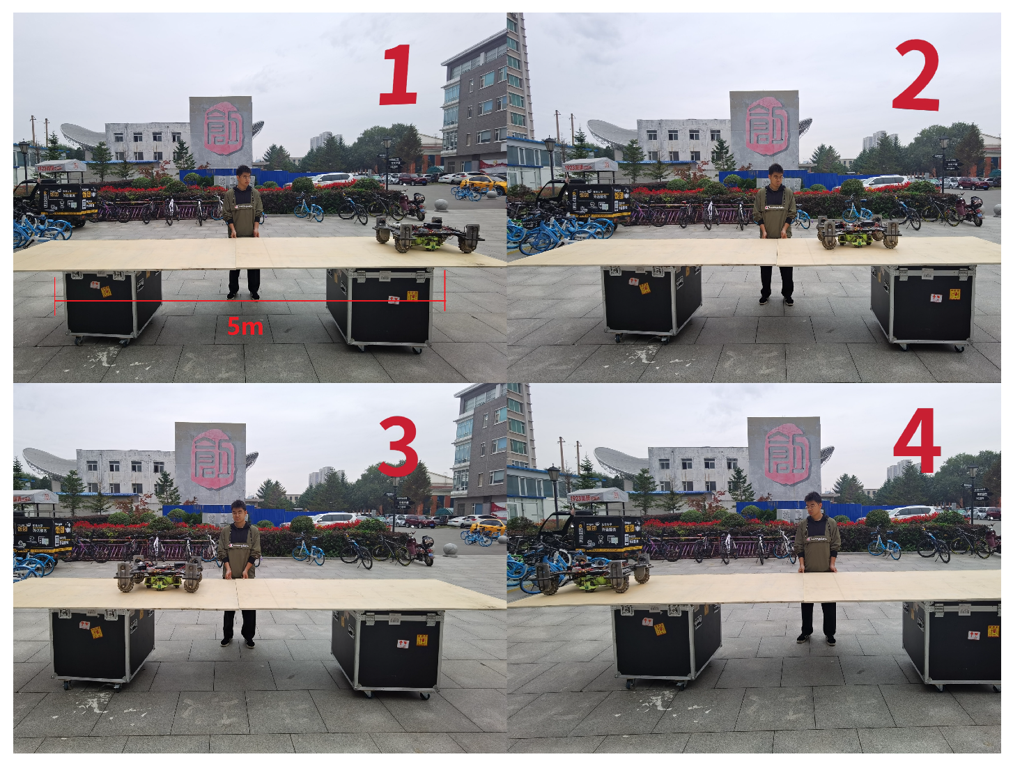
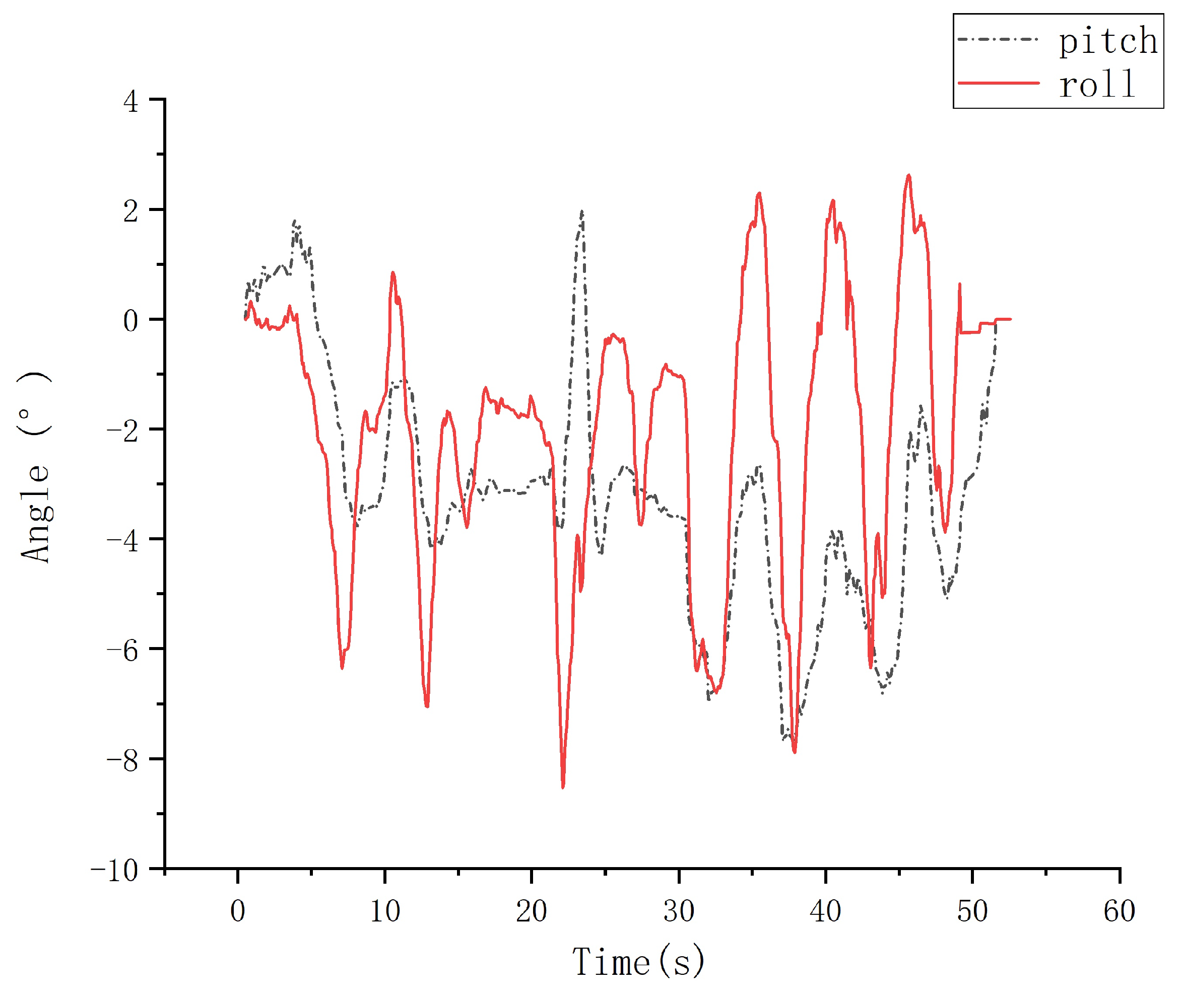
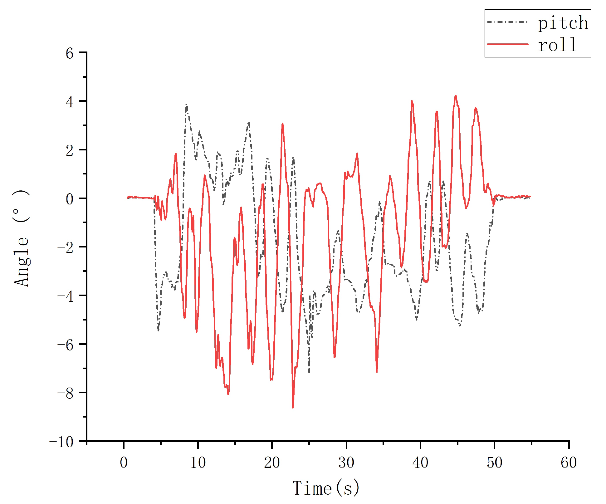
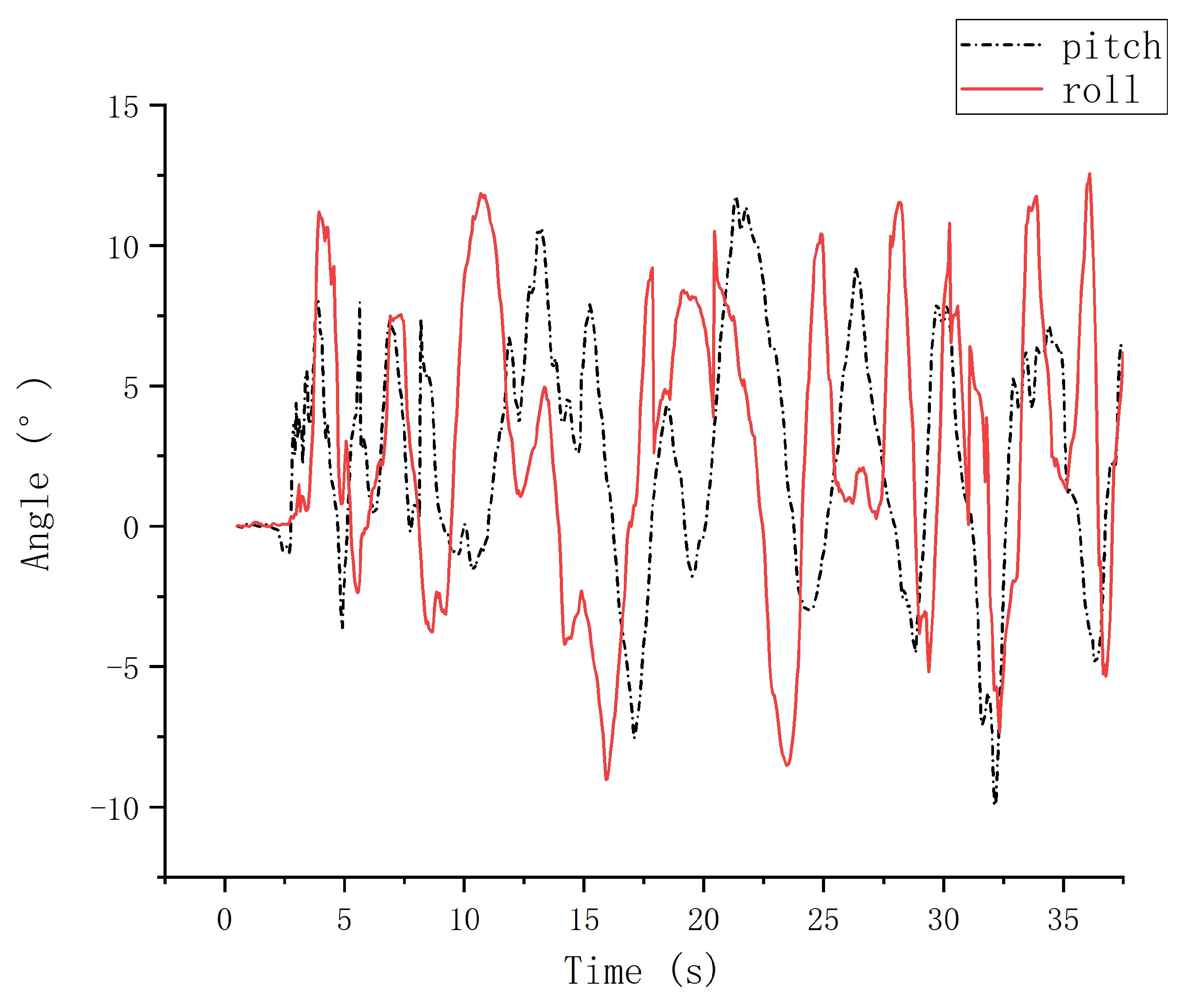
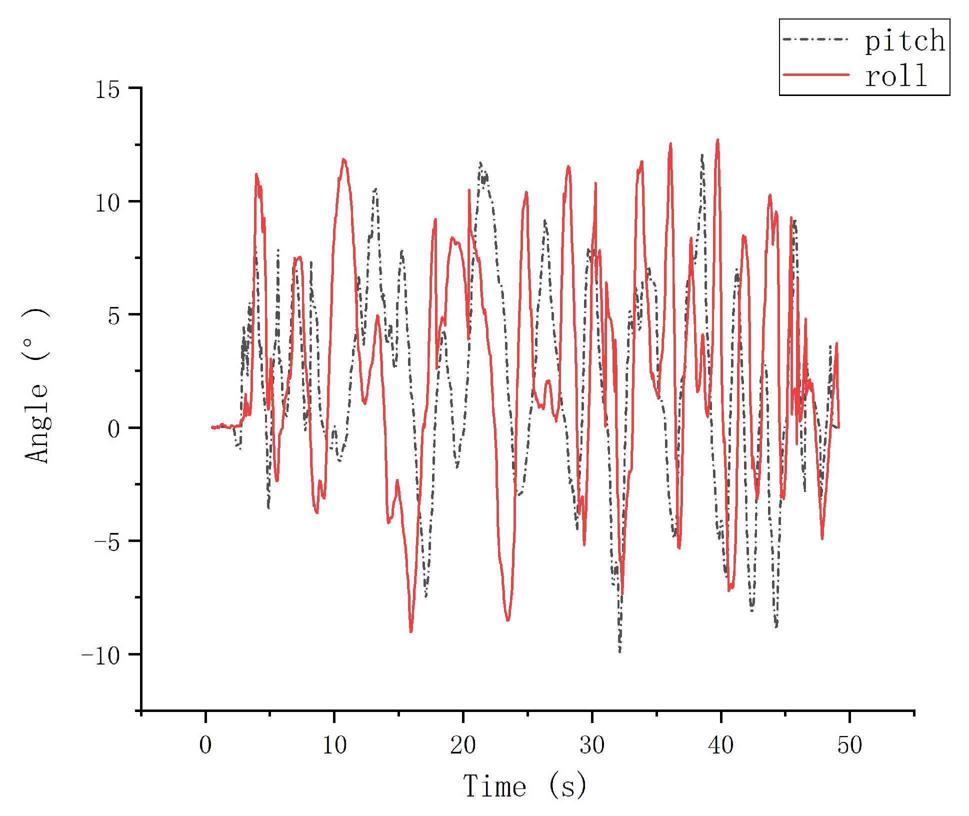
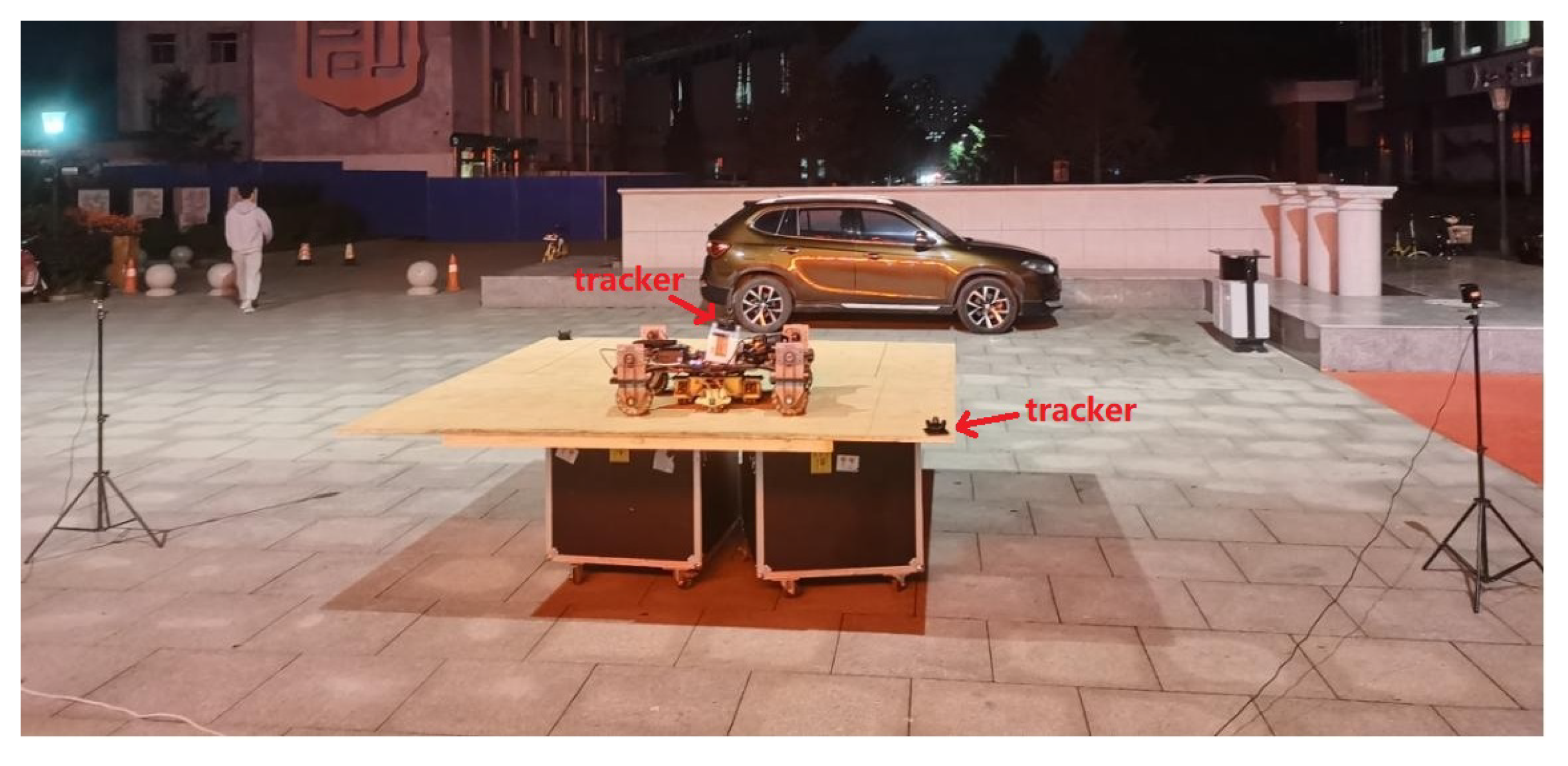
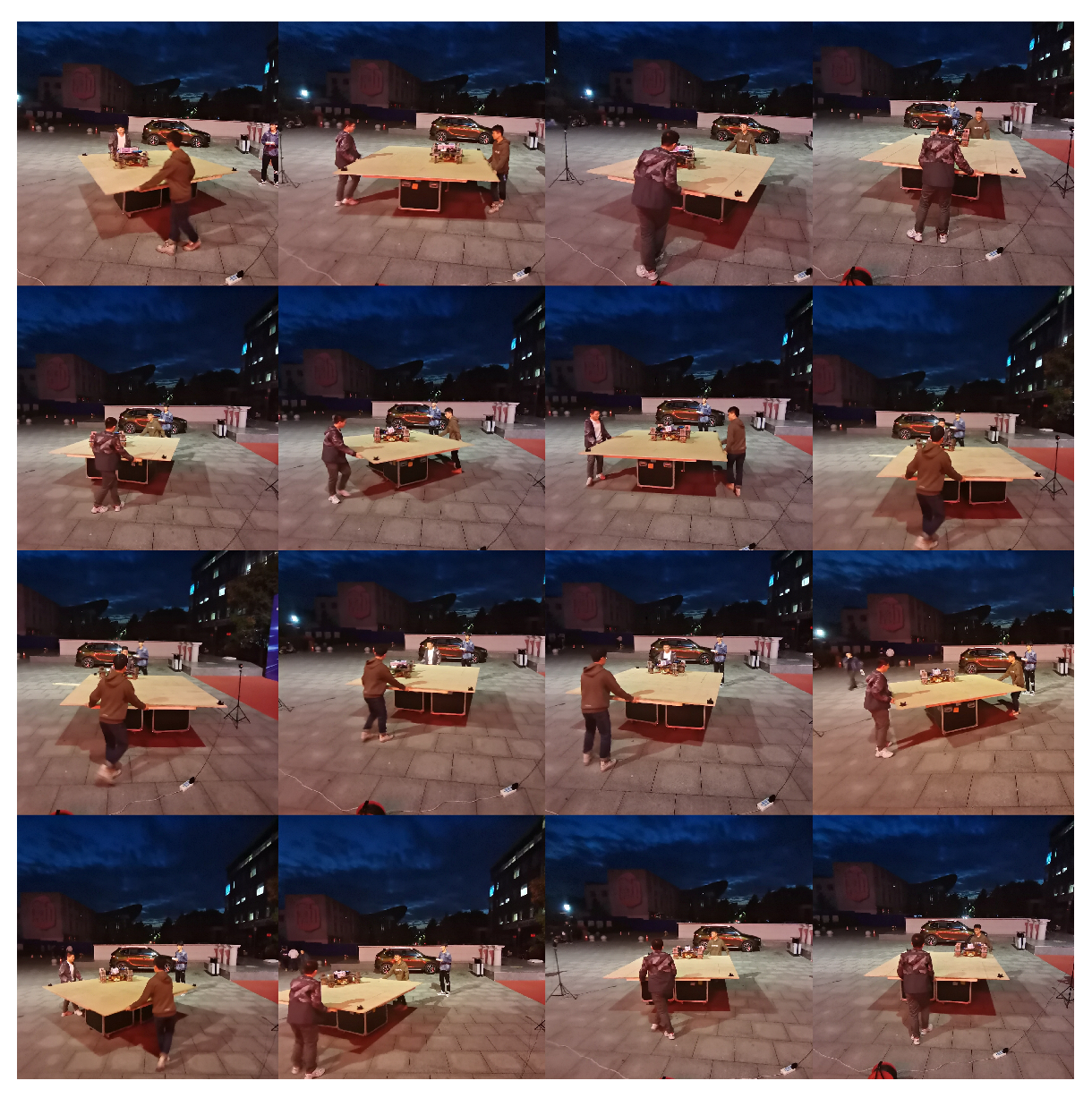
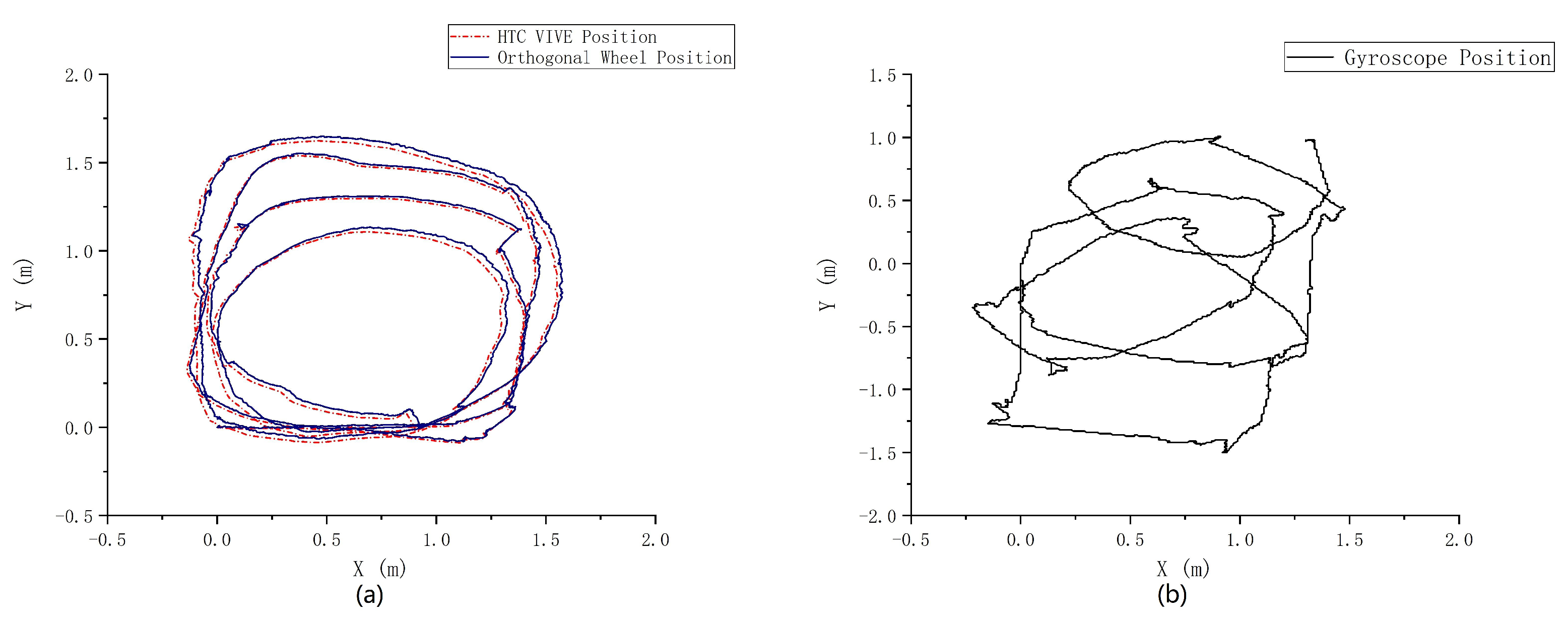
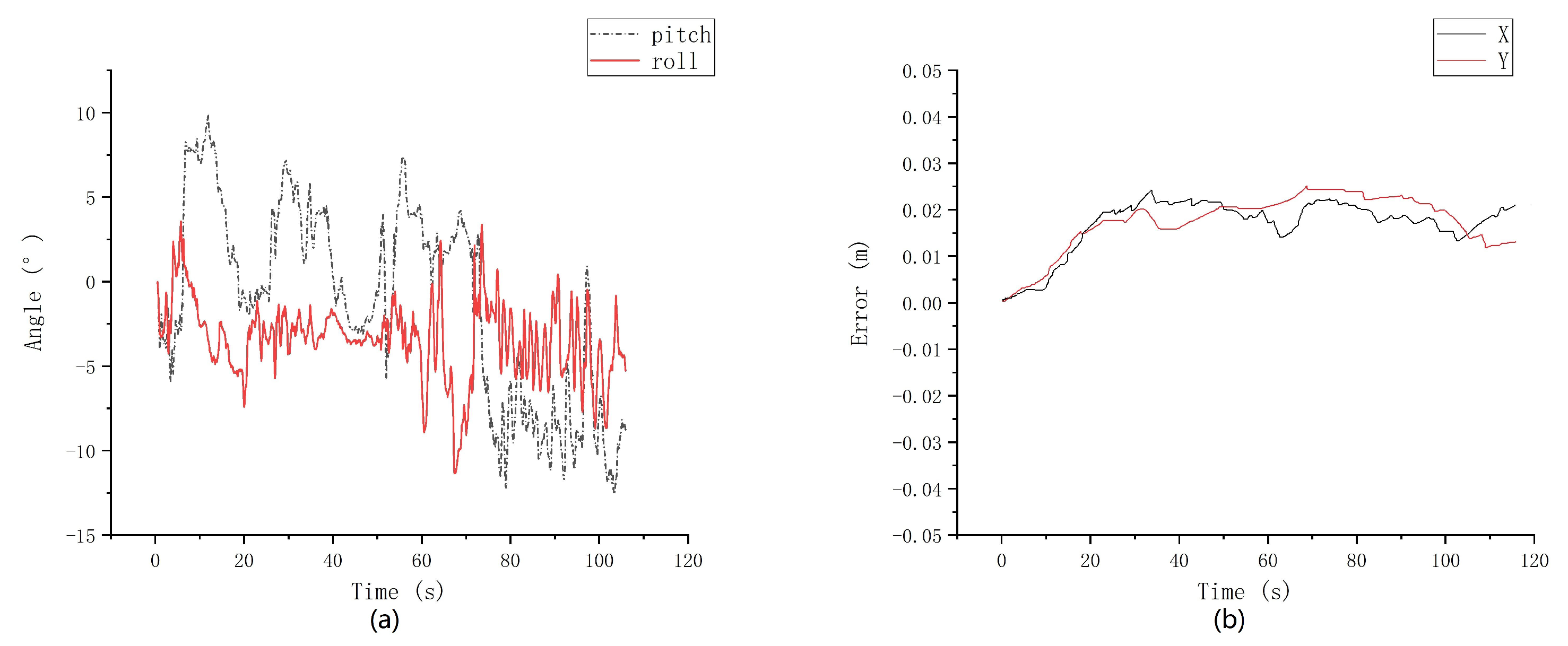
3.4. Simulated Floating Deck Experiment

The orthogonal wheels positioning system is designed at the beginning to deal with the common positioning methods, such as a gyroscope on the ship deck and other floating carriers, which do not have a good positioning effect. The environment of the above experiments is a fixed world coordinate system. In the world coordinate system, through the above experiments, we can verify the positioning accuracy and robustness of the orthogonal wheel positioning system in the absolute coordinate system. Next, the relative coordinate system experiment is carried out on the simulated floating deck experimental platform. Because the experimental scenes, such as the hull deck, are not convenient to obtain, the platform as shown in Figure 31 is adopted as the floating platform for this experiment. The floating hull is simulated by people lifting the plank and walking around at random. The floating platform is fitted with universal wheels to simulate the movement of the deck at sea.

On the floating test platform, the desired motion curve should be the actual curve of the positioning system relative to the floating test platform, not the actual curve in the world coordinate system. The tracker reflects the x, y, z coordinates and yaw, pitch, roll angles of the current moment relative to the world coordinate system. So we put a tracker on the moving chassis and a tracker on the corner of the platform. Through the tracker on the chassis, we can obtain the coordinates $\left(x,y\right)$ of the chassis in the world coordinate system at every moment. Through the tracker fixed in the corner of the platform, we can obtain the coordinates $\left(x_T,y_T\right)$ of the origin of the floating platform coordinate system in the world coordinate system and the rotation angle $\theta$ of the floating platform coordinate system in the world coordinate system at every moment. The position of a point $\left(x,y\right)$ in world coordinates in relative coordinates $\left(x^{\prime },y^{\prime }\right)$ is:

$$\left[\begin{array}{c}{x}^{\prime }\\ y^{\prime }\end{array}\right]=\left[\begin{array}{cc}cos\theta & sin\theta \\ -sin\theta & cos\theta \end{array}\right]\left[\begin{array}{c}x\\ y\end{array}\right]+\left[\begin{array}{c}{x}_T\\ y_T\end{array}\right]$$

The actual curve of the moving chassis relative to the floating platform can be obtained by the above method. Then the positioning curve is compared with that of the orthogonal wheel positioning system developed by ourselves. Figure 32 shows the actual process of this floating platform experiment. Two students control the floating platform to move irregularly, during which they shake the floating platform up and down to produce a floating effect. Another student remotely controls the chassis, moving around the floating platform in an irregular circle.

Figure 33a shows the motion track of the orthogonal wheel positioning system and HTC VIVE positioning system on the mobile floating platform. Figure 33b reflects the trajectory of the gyroscope positioning in this case.

As can be seen from the figure, the positioning curve of the orthogonal wheel positioning system tends to be consistent with the real curve of HTC VIVE. In the process of floating motion, the angle read by the gyroscope is not that of the orthogonal wheels relative to the floating platform, but that of the world coordinate system. As a result, the curve of the gyroscope positioning is unpredictable and inconsistent with the actual motion curve.

Figure 34 shows that the floating degree of the mobile floating platform and the error curve of the orthogonal wheel positioning system relative to HTC VIVE in the process of movement. On the mobile floating platform used in this experiment, the maximum error is 2.43 (±0.075) cm. According to the experimental data, the RMSE of the positioning system on the floating platform is 1.51 cm.

4. Discussion

As far as we know, previous studies have not focused much on floating surfaces, such as decks. For the wheeled positioning of robots, a gyroscope is the current, preferred method used for the angle measurement in terms of economy and practicality. The usual odometer system does have the biggest problems with turns and orientation changes. However, our positioning system is a mechanical structure design, and the calculation of the position when turning is mainly dependent on the radius of rotation of the structure. This is a fixed value, and as long as the radius of rotation is accurate, the error tends to zero. There is no sensor like the gyroscope: the more turns, the greater the angle deviation. Different from other commonly used odometers, the error of self-developed orthogonal wheel odometers fundamentally depends on whether the rotation radius and our orthogonal wheel radius are accurate, as well as the accuracy of the encoder to read the orthogonal wheel mileage.

Compared with the orthogonal wheel positioning system developed by ourselves, both LiDAR and gyroscopes have their drawbacks. The use of gyroscope is usually limited to the fixed plane based on the world coordinate system. With the increase in the gyroscope angle, the error also increases. In order to ignore the angle cumulative error of the gyroscope, the influence on the positioning error is minimal only in the case of a small number of turns. Laser positioning of LiDAR [23] is similar to the positioning mode of HTC VIVE used in the experiment. Although it has very high positioning accuracy, it has high requirements for the environment. In the process of LiDAR positioning, it is necessary to scan the surrounding environment and then match the boundary on the map to achieve the positioning effect. However, on a wide deck, it is hard to scan the boundaries we want, and it is even harder to locate them when there are dynamic obstacles. So LiDAR has its drawbacks, especially in the case of wide decks with unclear boundaries or sea fog. This new positioning technology needs to have accurate positioning accuracy and adaptability to floating environment. In view of the floating motion environment and the desired positioning task, the orthogonal wheels positioning sensor system designed by us can achieve a satisfactory positioning effect in this kind of environment.

According to the experiment in the third chapter, we can understand that the positioning effect of the orthogonal wheels positioning system can achieve a very high positioning accuracy during the movement of a certain distance, and the positioning error can reach within 0.025 m. It can be seen from the random comparison curve that the positioning curve of the orthogonal wheel positioning system is basically consistent with that of HTC VIVE, and the maximum error is 2.43 (±0.075) cm in the process of moving. The RMSE of the positioning system on the floating platform is 1.51 cm. However, the positioning curve of the positioning system using gyroscope deviates more and more with the progress of the movement. This is because the orthogonal wheels are driven by design, and the positioning mode of the orthogonal wheel positioning system is not affected by the error caused by rotation like the gyroscope. Additionally, the orthogonal wheel structure is equipped with a sliding structure so that the positioning system can easily ignore the irregular movement of the system caused by the floating ground. The experimental results show that the errors of the orthogonal wheel positioning system are within the acceptable range (±3 cm) under the conditions of linear motion, curvilinear motion and floating environment, and the expected effect of the centimeter-level positioning system is achieved. The experimental results highlight the potential application of the positioning system in a complex environment. In the case of subsequent use of other positioning calibrations, the accuracy may be even higher.

5. Conclusions and Future Work

This paper introduces a plane positioning sensor system based on orthogonal wheels and encoders. By using the characteristics of the orthogonal wheels of the system, we designed a new structure. The position and angle information of the mobile robot is obtained by solving the encoder installed on four sets of omnidirectional wheels. The system is designed to be an independent, economical, and easy-to-use customized solution for a ground that may be floating. It can obtain the desired position information that we want on any surface where floating occurs (such as ship decks, jolting cars or trains). In view of the current use of the IMU gyroscope positioning method, we use the experiment to prove its limitations. Due to the vertical sliding mechanism on each orthogonal wheel, the positioning system can easily face the irregular up and down movement of the system caused by the floating ground. In addition, it can solve the mismatch between the positioning data of the IMU odometer and the data in the world coordinate system under the floating ground condition. The experiment shows that the error of the positioning system is within the allowable range under the condition of linear and curved motion, and the expected effect is achieved.

In future work, on the basis of using the positioning system, we will continue to study the fusion of multi-sensor positioning, such as RFID, visual tags and so on, to make the positioning effect more obvious. In addition, we will consider using the fused localization sensor system to realize the functions of SLAM mapping and navigation. Using the positioning system as an odometer for map navigation in different environments should have better results.

References

1. Graham, J.D. An Audience of the Scientific Age: Rossum’s Universal Robots and the Production of an Economic Conscience. Grey Room 2013, 50, 112–142. [Google Scholar] [CrossRef]
2. Minsky, M.L. The emotion machine: Commonsense thinking, artificial intelligence, and the future of the human mind. Encycl. Neurol. Sci. 2008, 11, 15–17. [Google Scholar]
3. Tabarelli, D.; Vilardi, A. Statistically robust evidence of stochastic resonance in human auditory perceptual system. Eur. Phys. J. B 2009, 1, 155–159. [Google Scholar] [CrossRef]
4. Kube, C.R.; Vilardi, A. Task Modelling in Collective Robotics. Auton. Robot. 1997, 4, 53–72. [Google Scholar] [CrossRef]
5. Rosenberg, L.B. Virtual fixtures: Perceptual tools for telerobotic manipulation. In Proceedings of the IEEE Virtual Reality International Symposium, Seattle, WA, USA, 18–22 September 1993; pp. 76–82. [Google Scholar]
6. Wilson, A.R. Boston Dynamics introduces next generation humanoid robot. Vis. Syst. Des. 2016, 21, 53–72. [Google Scholar]
7. Zhang, S.; Xie, L.; Adams, M. An efficient data association approach to simultaneous localization and map building. In Proceedings of the IEEE International Conference on Robotics & Automation, Barcelona, Spain, 18–22 April 2005; Volume 24, pp. 49–60. [Google Scholar]
8. Cheng, Y.H.; Zhang, C.L. Mobile Robot Obstacle Avoidance Based on Multi-Sensor Information Fusion Technology. Appl. Mech. Mater. 2014, 2958, 490–491. [Google Scholar] [CrossRef]
9. Sugihara, K.; Smith, J. Genetic algorithms for adaptive motion planning of an autonomous mobile robot. In Proceedings of the IEEE International Symposium on Computational Intelligence in Robotics & Automation, Monterey, CA, USA, 10–11 July 1997. [Google Scholar]
10. Borio, D.; Closas, P. Robust transform domain signal processing for GNSS. Navigation 2019, 66, 305–323. [Google Scholar] [CrossRef] [Green Version]
11. Borio, D.; Closas, P. A Pseudolite-Based Positioning System for Legacy GNSS Receivers. Sensors 2014, 4, 6104–6123. [Google Scholar]
12. Tu, R.; Zhang, R. Real-time detection of BDS orbit manoeuvres based on the combination of GPS and BDS observations. IET Radar Sonar Navig. 2020, 10, 1603–1609. [Google Scholar] [CrossRef]
13. Fujii, K.; Sakamoto, Y. Hyperbolic Positioning with Antenna Arrays and Multi-Channel Pseudolite for Indoor Localization. Sensors 2015, 10, 25157–25175. [Google Scholar] [CrossRef] [Green Version]
14. Zhao, Y.; Peng, Z. A New Method of High-Precision Positioning for an Indoor Pseudolite without Using the Known Point Initialization. Sensors 2018, 18, 1977. [Google Scholar] [CrossRef] [Green Version]
15. Stavrou, V.; Bardaki, C.; Papakyriakopoulos, D.; Pramatari, K. An Ensemble Filter for Indoor Positioning in a Retail Store Using Bluetooth Low Energy Beacons. Sensors 2019, 19, 4550. [Google Scholar] [CrossRef] [Green Version]
16. Kwangjae, S.; Dong, L.; Hwangnam, K. Indoor Pedestrian Localization Using iBeacon and Improved Kalman Filter. Sensors 2018, 18, 1722. [Google Scholar]
17. Xin, L.; Jian, W.; Liu, C. A Bluetooth/PDR Integration Algorithm for an Indoor Positioning System. Sensors 2015, 15, 24862–24885. [Google Scholar]
18. Ferreira, A.; Matias, B.; Almeida, J.; Silva, E. Real-time GNSS precise positioning: RTKLIB for ROS. Int. J. Adv. Robot. Syst. 2020, 17, 1729881420904526. [Google Scholar] [CrossRef]
19. Zhang, H.; Zhang, C.; Wei, Y.; Chen, C.Y. Localization and navigation using QR code for mobile robot in indoor environment. In Proceedings of the IEEE International Conference on Robotics & Biomimetics, Zhuhai, China, 6–9 December 2015. [Google Scholar]
20. Duque Domingo, J.; Cerrada, C.; Valero, E.; Cerrada, J.A. An Improved Indoor Positioning System Using RGB-D Cameras and Wireless Networks for Use in Complex Environments. Sensors 2017, 17, 2391. [Google Scholar] [CrossRef] [Green Version]
21. Xu, H.; Ding, Y.; Li, P.; Wang, R.; Li, Y. An RFID Indoor Positioning Algorithm Based on Bayesian Probability and K-Nearest Neighbor. Sensors 2017, 17, 1806. [Google Scholar] [CrossRef] [Green Version]
22. Guarato, F.; Laudan, V.; Windmill, J.F.C. Ultrasonic sonar system for target localization with one emitter and four receivers: Ultrasonic 3D localization. In Proceedings of the 2017 IEEE SENSORS, Glasgow, Scotland, 29 October–1 November 2017. [Google Scholar]
23. Kim, H.; Liu, B.; Myung, H. Road-feature extraction using point cloud and 3D LiDAR sensor for vehicle localization. In Proceedings of the 2017 14th International Conference on Ubiquitous Robots and Ambient Intelligence (URAI), Jeju, Korea, 28 June–1 July 2017. [Google Scholar]
24. Wang, B.; Liu, X.; Yu, B.; Jia, R.; Gan, X. An Improved WiFi Positioning Method Based on Fingerprint Clustering and Signal Weighted Euclidean Distance. Sensors 2019, 19, 2300. [Google Scholar] [CrossRef] [Green Version]
25. Chen, G.; Meng, X.; Wang, Y.; Zhang, Y.; Tian, P.; Yang, H. Integrated WiFi/PDR/Smartphone Using an Unscented Kalman Filter Algorithm for 3D Indoor Localization. Sensors 2015, 15, 24595–24614. [Google Scholar] [CrossRef] [PubMed] [Green Version]
26. Zou, H.; Lu, X.; Jiang, H.; Xie, L. A Fast and Precise Indoor Localization Algorithm Based on an Online Sequential Extreme Learning Machine. Sensors 2015, 15, 1804. [Google Scholar] [CrossRef] [PubMed]
27. Willemsen, T.; Keller, F.; Sternberg, H. Concept for building a MEMS based indoor localization system. In Proceedings of the International Conference on Indoor Positioning & Indoor Navigation, Busan, Korea, 27–30 October 2014. [Google Scholar]
28. Eyobu, O.S.; Poulose, A.; Han, D.S. An Accuracy Generalization Benchmark for Wireless Indoor Localization based on IMU Sensor Data. In Proceedings of the 2018 IEEE 8th International Conference on Consumer Electronics, Berlin, Germany, 2–5 September 2018. [Google Scholar]
29. Gan, X.; Yu, B.; Huang, L.; Jia, R.; Zhang, H.; Sheng, C.; Fan, G.; Wang, B. Doppler Differential Positioning Technology Using the BDS/GPS Indoor Array Pseudolite System. Sensors 2019, 19, 4580. [Google Scholar] [CrossRef] [PubMed] [Green Version]
30. HTC Vive. China Releases First Self-Developed Group Standard for the VR Industry. Electronics Newsweekly, 25 April 2017; p. 74.
Figure 1. Physical picture of the positioning system.
Applsci 11 11340 g001
Figure 2. (a) Physical picture of encoder and slave wheel installation. (b) Physical drawing of sliding mechanism. The range of up and down movement is 6 cm. Every sliding mechanism supports the amount of ground unevenness at ±3 cm.
Applsci 11 11340 g002
Figure 3. A 3D diagram of positioning sensing system.
Applsci 11 11340 g003
Figure 4. Main view and left view of a single orthogonal omnidirectional wheel.
Applsci 11 11340 g004
Figure 5. (a,b) The status of the sliding mechanism of the positioning system before and after complete pressure, respectively, which can withstand a movement of approximately 6 cm up and down. (c) The positioning system can still maintain contact with the ground under the plane simulating the inclined ground. From the positioning system structure, the maximum allowable slope is approximately 15°.
Applsci 11 11340 g005
Figure 6. The motion model of single omnidirectional wheel in world coordinate system and self coordinate system.
Applsci 11 11340 g006
Figure 7. The motion model of four omnidirectional wheels in world and its own coordinates. The horizontal plane body coordinate system XOY: the center of the body is the center point O, OX direction is the direction of the moving robot, OY direction is the vertical direction of the moving robot. The initial position coordinates of the mobile robot (x, y) are the origin of the world coordinate system.
Applsci 11 11340 g007
Figure 8. The magnetic encoders on the four omnidirectional wheels transmit the data to the CPU respectively. After data processing by the central processor, the position information is transmitted to the upper computer through serial port.
Applsci 11 11340 g008
Figure 9. Data from the encoders on the two orthogonal wheels and a gyroscope converted by AD are transmitted to the CPU respectively. After data processing by the CPU, the position information is transmitted to the upper computer through serial port.
Applsci 11 11340 g009
Figure 10. (a) The mobile chassis platform used in this experiment. (b) The self-developed positioning system is mounted under the mobile chassis.
Applsci 11 11340 g010
Figure 11. The chassis coordinate diagram of mobile robot. In the figure, P is the origin of the vehicle’s own coordinate system, and O is the origin of the world coordinate system.
Applsci 11 11340 g011
Figure 12. Simulation floating experimental platform, size of 5.4 m × 1.3 m.
Applsci 11 11340 g012
Figure 13. The motion of the chassis in the X direction. The motion distance is 5 m.
Applsci 11 11340 g013
Figure 14. The actual motion scene in the X direction. In the figure, 1, 2, 3 and 4 are the four stages of the movement process respectively.
Applsci 11 11340 g014
Figure 15. (a) The change curve of displacement when the mobile robot travels once along the X direction. (b) The displacement curve of the mobile robot when it repeats three times along the Y axis.
Applsci 11 11340 g015
Figure 16. The angle of chassis coiling around pitch and roll axis.
Applsci 11 11340 g016
Figure 17. The actual motion scene in the Y direction. The motion distance is 5 m. In the figure, 1, 2, 3 and 4 are the four stages of the movement process respectively.
Applsci 11 11340 g017
Figure 18. The displacement curve of the mobile robot when it repeats four times along the Y axis.
Applsci 11 11340 g018
Figure 19. The angle of chassis coiling around pitch and roll axis.
Applsci 11 11340 g019
Figure 20. The actual motion scene of the chassis rotation. In the figure, 1, 2, 3 and 4 are the four stages of the movement process respectively.
Applsci 11 11340 g020
Figure 21. (a) The angle change curve of the mobile robot when it rotates continuously for two turns along the Z axis. (b) The angle change curve when the mobile robot rotates one circle counterclockwise and one circle clockwise along the Z axis.
Applsci 11 11340 g021
Figure 22. The angle of chassis coiling around pitch and roll axis.
Applsci 11 11340 g022
Figure 23. Simulation floating experimental platform, size of 2.4 m × 2.4 m.
Applsci 11 11340 g023
Figure 24. The movement track of the mobile chassis. The length of the square side is 1.8 m. The four points of the square are set to P 0 , P 1 , P 2 , and P 3 . In the horizontal plane coordinate system XOY, the center of the chassis is center point O, OX direction is the initial motion direction of the mobile chassis, and OY direction is the vertical direction of moving robot. The initial position coordinates of the mobile robot (x, y) are the origin of the world coordinate system.
Applsci 11 11340 g024
Figure 25. The actual motion scene. In the figure, 1, 2, 3 and 4 are the four stages of the movement process respectively.
Applsci 11 11340 g025
Figure 26. (a) Comparison diagram of actual motion curve and theoretical motion curve. The actual motion curve is basically consistent with the preset motion path. (b) The angle change curve of the mobile robot when it moves in a counterclockwise direction along a square.
Applsci 11 11340 g026
Figure 27. The angle of chassis coiling around pitch and roll axis.
Applsci 11 11340 g027
Figure 28. The site layout of the laboratory. HTC VIVE2.0 base stations are placed on both sides of the site, and the base stations are placed on the same axis with a height of one meter.
Applsci 11 11340 g028
Figure 29. The tracker is fixed in the center of the moving chassis, which is the center of the orthogonal wheels system.
Applsci 11 11340 g029
Figure 30. (a) Comparison diagram of the gyroscope position curve, orthogonal wheels position curve and HTC VIVE position curve. (b) The error curve of orthogonal wheel relative to HTC VIVE.
Applsci 11 11340 g030
Figure 31. Simulated floating deck experimental platform. The size of the experimental platform is 2.4 m × 2.4 m. Place a tracker in the center of the chassis and in the corner of the platform.
Applsci 11 11340 g031
Figure 32. The actual process of this floating platform experiment.
Applsci 11 11340 g032
Figure 33. (a) The motion curve of the orthogonal wheels in irregular motion with the mobile floating platform. Compared with the actual curve, the orthogonal wheel positioning system has a good positioning effect relative to the moving path of the mobile floating platform. (b) Motion curve of gyroscope positioning along with irregular movement of the floating experimental platform. With the accumulation of angle errors in the process of motion, the obtained motion curve becomes more and more yaw.
Applsci 11 11340 g033
Figure 34. (a) The angle of chassis coiling around pitch and roll axis. (b) The error curve of orthogonal wheel relative to HTC VIVE.
Applsci 11 11340 g034