Dynamic Process Simulation of a Molten-Salt Energy Storage System

Abstract

The main objective of this work was the construction of a numerical model using Advanced Process Simulation Software to represent the dynamic behaviour of a thermal storage system (TSS). The storage model was validated by comparing the results with the measured data of the storage process of the Andasol 2 solar power plant. Subsequently, a system analysis and system optimisation were carried out, and the stand-alone concept of the thermal storage system is presented. Stand-alone refers to an isolated use of the storage system without a solar power plant. During power peaks, this storage medium is heated with excess electrical power and later returned to the electrical grid through a steam cycle. Then, the system was optimised by modelling four models based on the type of storage medium and the temperature difference of the storage system. The four models, Andasol 2, SSalt max, Hitec, and Carbonate, were evaluated and compared in terms of the improvement in capacity and efficiency that can be achieved. The comparison shows that the preferred storage medium is carbonate salt due to the increases in both efficiency and capacity. The greatest increase in efficiency in terms of power generation can also be achieved with the Carbonate model (18.2%), whereas the amount of increase was 9.5% and 7.4% for each of SSalt max and Hitec, respectively. The goal of this analysis and system optimisation of a thermal salt storage system is to stabilise and relieve the local power grid.

1. Introduction

The depletion of fossil fuels and the increasing number of problems caused by global warming have increased interest in renewable energy sources in recent years [1]. At present, 46% of the electricity generated in Germany is obtained from renewable energy sources. As a result of the increasing share of sustainable power generation, the load on the power grid has increased because such power generation has significant dependencies on meteorological influences. In order to enable a further expansion of renewable energy sources, it is necessary to relieve and stabilise the power supply through the use of energy storage devices.

Energy storage is divided into electrical, chemical, mechanical and thermal energy storage according to its operating principle [2]. Electrical storage uses electrical and magnetic fields to store energy (for a short time). Chemical storage is the storage of energy with the help of material energy carriers [3]. In electrochemical storage systems, the stored energy is in chemical form in the electrodes. These also act as energy stores and converters. They have a fast response time, but have a short lifespan (<10 years) and show a constant loss of capacity. Mechanical storage uses the forced change in position (potential), speed (kinematics) or the thermodynamic state (pressure) of a material to store energy [4].

Thermal energy storage is discussed as the last operating principle, and can be divided into three types of thermal storage: latent, thermochemical, and sensitive. It is expected that thermal storage will gain increasing importance in the future because the heating sector is the largest energy sector in Europe, accounting for approx. 50% of energy consumption [1].

The most important type of energy storage for this work is that of sensible heat storage. In this type, heat is stored based on temperature difference. More precisely, a medium is heated during charging in order to absorb (excess) heat, and cooled during discharging, or the thermal energy is removed again. In sensible heat storage, the heat capacity of the storage medium, the mass, and the temperature difference are important. Furthermore, effective thermal insulation is essential, especially for long-term storage. Because of its low price and high level of development, it is currently the most common form of heat storage.

Thermal salt storage systems are currently used in a large number of solar power plants to ensure a constant power supply even though the solar radiation fluctuates in daylight and disappears during the night. The research and development of these storage systems are currently largely limited to steady-state process simulation models [5]. These do not require any control structures and are mathematically based on mass, momentum, and energy balances, which simplifies the initial system description. However, the transient and continuous changes in operating conditions can influence the efficiency of the investigated power plant. A recent literature review shows that there are few studies regarding the optimisation of the parabolic trough power plant employing dynamic and steady-state models.

A high temperature storage model of a solar tower power plant can be explained with open volumetric receiver technology using air as the heat transfer fluid (HTF) [6]. The model of the storage system was designed in the MATLAB/Simulink. The type of storage system investigated in this study is a bed-packed thermal energy storage system that has regeneration properties. It was used to develop various models of thermal storage systems using the lumped parameter method. First, the implemented models were stimulated to achieve high accuracy for the obtained results. Second, the dynamic properties of the thermal storage systems were extensively evaluated by applying turbulence of 15% to the mass flow. The results indicate that the charge and discharge properties of the three developed storage models have the same behaviour [7]. A dynamic solar field (SF) and thermal storage system (TSS) model of a 1 MW solar tower power plant was implemented in Beijing using Modelica software. The transient behaviour of charge storage and release processes for inlet and outlet steam quality was tested [8]. A proposed model was designed to provide a complete simulation of a thermocline tank operated at the lowest computing cost and to address the shortcomings of models developed in the previous studies. The suggested model was then integrated into a system-level model of a 100 MW_el solar tower power plant to study the storage capability in long-term service. The heliostat array and solar absorber tubes were modelled using DELSOL software, whereas the transient absorber tubes response was simulated using SOLERGY software. The study showed that the efficiency of the thermocline tank in accumulating and releasing thermal energy is approximately 99% year-round. Despite the excellent level of thermal efficiency, the structural stability of the thermocline tank remains a problem due to the high thermal expansion of the internal quartzite stone at high temperatures of the molten salt [9]. A 50 MW_el parabolic trough power plant has been modelled with (TRNSYS© software, 2007). Two heat transfer fluids (thermal oil and molten salt) were applied in this model. Seven operation strategies for charging and discharging modes were analysed to determine the most appropriate mode of operation that will minimise the difference in annual return between the two systems [10]. A parabolic trough power model was developed using APROS. A precise specification of the control response structures and operating approach was implemented to ensure appropriate dynamic performance. The operating strategies used in this model were also proven to be effective in enhancing power plant output and improving power plant operating hours using TSS compared to the operator’s choices under cloudy sky conditions [11]. The periodic processes of molten salt storage system thermoclines for parabolic trough solar plants were systematically evaluated using two temperature models. These models were designed by Fluent 6.1 and investigated with measured data. It was found that cycle efficiency is improved for smaller Reynolds numbers of molten salt, larger aspect ratios (distance of flow of molten salt in half a cycle relative to the diameter of the filler particles), and larger tank height. It was shown that the diameter of the filler particles and the capacity of the tank significantly affect the efficiency of the cycle [12]. A ceramic honeycomb TSS was modelled for a 10 kW solar air Brayton cycle system in this study using steady-state cycle analysis. The TSS showed very good operational efficiencies under the charge and discharge experimental tests, which were 79.6% and 76.5%, respectively. This study provides a contribution to the designing and modelling of TSS for solar-air Brayton cycle systems and to the analysis of the power plant operation strategy [13]. The binary nitrate (KNO₃ + Ca (NO₃)₂) with a melting point of 116.9 °C was chosen as the heat storage media in this research. The objective of this study was to achieve a stable and constant heat discharge performance of the TSS with a single tank of molten salt. A comparative study was undertaken of three different inlet velocity conditions, such as a steady value, automatic adjustment, and manual adjustment. According to the results, the heat discharge power decreases with increasing heat discharge period at a constant inlet velocity. The heat discharge period reduces as the inlet velocity increases, but the heat discharge power increases as the inlet velocity increases. The heat discharge power under automatic and manual adjustment of inlet speed varies by ±3% and ±10% from the set value, respectively [14]. A numerical model was built using enthalpy porosity model and two-temperature energy equations to evaluate thermal energy storage, extract the latent thermal energy from a storage system, and understand detailed heat transfer properties during a phase change material. The results showed that coating molten salt with nickel foam to effectively improve the thermal conductivity of the phase change material can enhance the performance of these types of systems [15]. A mathematical model for simulating the thermal performance of the high-temperature latent heat storage system in concentrating solar power plants was proposed, and satisfactory agreements were obtained between the simulated results and the empirical measurements. It can be seen that the average charging and discharging rates are enhanced by 6.8% and 9.1%, respectively, and the total thermal storage efficiency of the latent heat storage system increases from 34.4% to 44.1% due to the installation of circular fins [16]. The optimal design and technical and economic analysis of the stand-alone hybrid energy system was addressed for a rural city in China. A composite integer linear optimisation model was proposed with the objective of minimum overall annual cost depending on the assessment of current domestic renewable energy capacity potential and the study of heat and electricity consumption behaviour [17].

In order to ensure a realistic view of the efficiency and a precise design of the process components, a dynamic representation of the system is required. The originality of this work can be summarised as follows: In this study, the dynamic model of a thermal salt storage facility was modelled in APROS. The purpose is thus to represent the reference process as precisely as possible and to analyse the possible system improvements by changing the storage medium, which therefore produces differences in temperature for each medium used. The most important problem addressed by this study is how to utilise the surplus electricity generated from renewable energy sources during molten salt heating to be used later for electricity generation. Subsequently, a system analysis and system optimisation was performed and the stand-alone concept of the thermal salt storage system is presented.

Here, the structure and further development of the model is discussed in detail using APROS and any assumptions and simplifications made are presented. The model was then validated by comparing it with the storage process of the Andasol 2 thermal power plant. After the model was validated, further storage fluids were inserted into the model in order to analyse them with regard to system optimisation. In the following sections, a description of the system, modelling and simulation, results, and conclusions are presented.

2. Description of the System

The combined cycle power plant system with a storage system consists of the water/steam paths, gas turbine section, and thermal storage system (TSS). The schematic representation of the combined cycle power plant with the thermal storage system (TSS) can be seen in Figure 1. In this work, the TSS is only implemented with hot and cold tanks connected via heat exchangers. Two working media (molten salt and heat transfer fluid (HTF)) are used in the TSS. Each of the two salt tanks has a diameter of 38.5 m and a height of 14 m. The total amount of molten salt used is about 28,500 t. The TSS and the process of charging and discharging are explained in more detail in the following sections.

2.1. Working Cycle

The working cycle of TSS can be divided into two operating periods of charge and discharge. In the charge period, the molten salt coming from the CST is heated by surplus electricity generated using any renewable energy sources, as shown in Figure 2. Then, the hot molten salt is stored in the HST. The charging process continues until the HST is completely filled or the surplus electricity from renewable sources is reduced.

During the charge period, on the one side, the air coming from the air compressor enters the heat exchanger of TSS, while on the other side the hot molten salt is pumped to the same heat exchangers in order to heat the airflow, as demonstrated in Figure 3. Then, the hot air enters the expander to generate electricity. After that, the expanded hot air flows into HRSG to complete the steam cycle with three pressure circuits. Thereafter, this process continues until the HST is completely depleted. It should be mentioned here that three types of molten salt will be used in this study.

2.2. Working Media

Due to the high costs compared to molten salt and the limited temperature range, salt storage is more commonly used. Therefore, this paper discusses the two main types of molten salt.

2.2.1. Liquid Salt

Liquid salt is the name given to salt compounds that are used above their melting point. The most widely used liquid salts for thermal storage in the industry are the nitrate salts Hitec and Solar Salt. Hitec is a ternary liquid salt (53% KNO₃, 40% NaNO₂, 7% NaNO₃) with a melting point of approx. 142 °C [18]. It can be operated up to 535 °C. At temperatures above 535 °C, it decomposes and becomes unusable for further use. Solar Salt is a binary nitrate salt (60% NaNO₃, 40% KNO₃). It can be operated from approx. 220 to 585 °C.

Due to the large temperature range in which liquid salts are used, they are particularly suitable for storing thermal energy. Compared with thermal oil, they are also cheaper, more readily available, and less harmful to the environment, Moreover, although thermal oil and molten salt have almost the same specific heat capacity, the density of molten salt is about twice as high. Therefore, with the same storage capacity, thermal oil storage tanks accordingly have a volume that is twice as large. The main difficulty with using molten salt is the risk of solidification. If the temperature falls below the melting point, the salt solidifies and the volume contracts, causing irreversible destruction of the system [19].

It must therefore be ensured at all times that the salt is constantly kept above its melting point at all points in the system.

2.2.2. Carbonate Salt

In order to work in temperature ranges of over 500 °C, carbonate salts instead of nitrate salts may be used in the future. These is not currently used as a storage medium and in this respect the level of development is very low. In a study by Wu, Ren, Wang and Ma [20], it was shown that carbonate salts are suitable as a high-temperature storage medium. More precisely, 36 carbonate salts were tested in the study, which differed only in the concentration of their three inorganic salts—K₂CO₃, Li₂CO₃, Na₂CO₃. The advantage of carbonate salts compared to nitrate salts is, as mentioned above, the working temperature. The melting temperature for the carbonate salt specified as optimal in [20] is 400 °C. The decomposition temperature is correspondingly higher (830 °C), which not only promises a greater temperature range than nitrate salt, but also a higher efficiency can be achieved when generating electricity later due to the high temperature [20]. It should be noted here that a carbonate salt storage facility can only be implemented as a direct storage facility, as there is currently no HTF that can be used in a temperature range of 400–850 °C. This means that the carbonate salt must be a storage medium and HFF at the same time. The specific heat capacity is discussed in more detail below when presenting the implementation of carbonate salt in APROS.

3. Modelling and Simulation

Following the above description of the working cycle, the modelling process and assumptions made are presented. First, the basic model is described, on which the further modelling is based. Then the weaknesses of the system are identified and the system is further developed. A distinction must be made between the process and the so-called automation. Both the process and the associated automation are APROS work areas. In the process, the physical components of the system are modelled (for example pumps, pipes, tanks, and valves). Signals and electrical components are displayed in automation. This includes the control and regulation of the system, but also signals and external influences, such as the power at which the system is charged by renewable energy sources. After the further development of the model, the validation follows. This checks how closely the simulation results align with subsequent practical results.

In this work, a one-dimensional, homogeneous two-phase pressure-flow model (referred to as a homogeneous model in APROS) was used. This is based on the dynamic conservation equations for mass, momentum and energy. APROS calculates the thermodynamic state from the known enthalpy, composition of the fluid, and pressure for each individual calculation node in each time step. From this, the respective node temperature, the gas volume fraction, the phase composition and the individual fluid properties, such as density, dynamic viscosity, and heat capacity, are calculated [21,22,23,24].

3.1. Basic Model

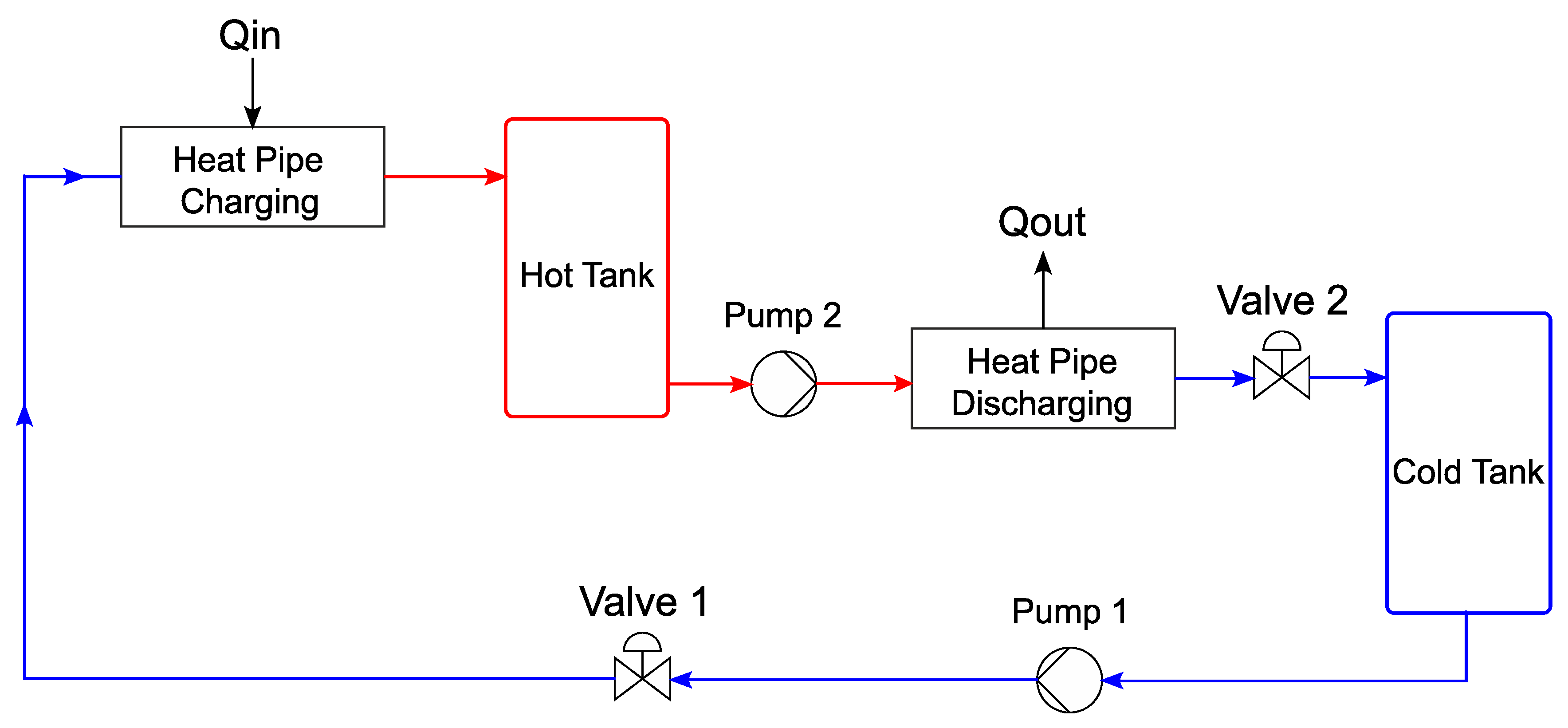
An APROS 6 model of a thermal storage tank was developed in this work and used as the basis for the modelling. The schematic structure of the basic thermal storage model can be seen in Figure 4. The model consists of two tanks (CST and HST), two valves (V₁ and V₂), two pumps (P₁ and P₂), and two heat exchangers (Q₁ and Q₂). The individual components are connected by pipes.

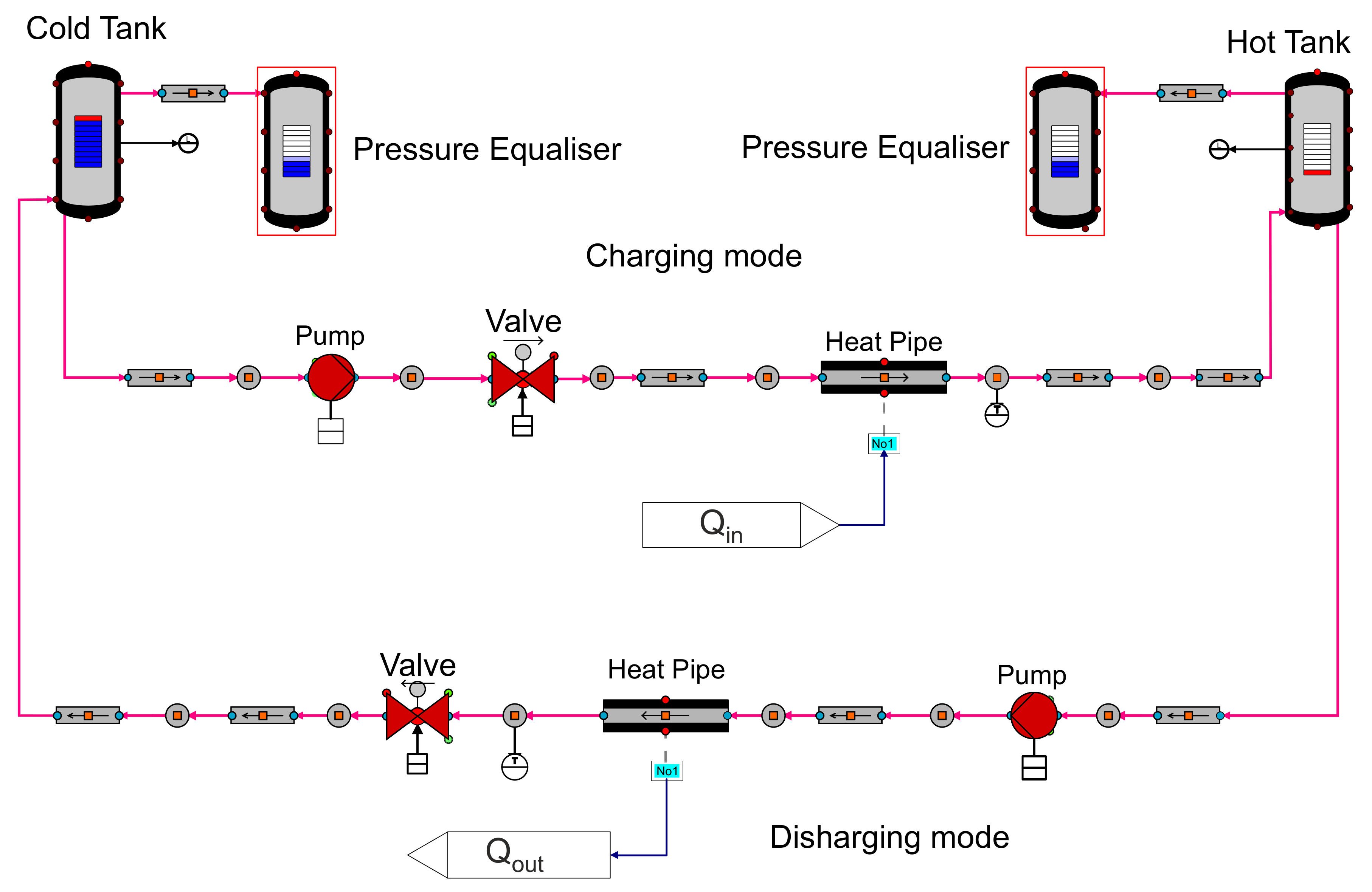
In contrast to Figure 1, the charging and discharging of the salt storage in the APROS model is realised with two different pipe systems. The reason for this is that APROS can only calculate flows in a certain direction. Thus, if the fluid in the same component is allowed to flow in the opposite direction, the simulation is aborted. However, the use of two different pipe systems instead of one should not affect subsequent results.

The salt storage tanks are modelled with the Heat_Tank component from the APROS library. The dimensions are taken as described above [25]. At an initial temperature of 282 °C, a temperature difference of 28 °C was determined over a period of six weeks with an outside temperature between 2 and 6 °C. This corresponds to a daily loss of 0.66 °C, which is negligible. The pumps are modelled with the BASIC_PUMP component. This defines the pump by the following five parameters: nominal flow rate, nominal delivery head, maximum delivery head, length, and flow cross-section.

The pump is controlled via the rotational speed, as a percentage, depending on the maximum speed. The power calculated from this assumes that the pump works isentropically [26].

The valves are modelled with the component CONTROL_VALVE. To fully define a valve, the program requires the following five parameters: valve length, flow cross-section, nominal mass flow, loss of nominal pressure, and nominal density.

The valves are controlled by their percentage of opening, where 100% represents a fully open valve.

The heat exchangers are modelled with the components HEAT_PIPE and BOUNDARY_CONDITION. With the component HEAT_PIPE, only a pipe with thermal insulation is initially implemented. The BOUNDARY_CONDITION is used to supply the fluid in the pipe with a heat flow in W_th in one or more nodes. In this case, the heat is transferred through three nodes. This promises a more accurate result than feeding through a single node. Alternatively, it would also be possible to model a countercurrent heat exchanger with an HTF mass flow on one side and the molten salt mass flow on the other. However, it would not be possible to precisely record the supplied thermal energy, which is essential for subsequent validation of the model. Unknown characteristic values are left at the standard value (from APROS) or modified according to the cycle process so that APROSdoes not display any error messages. After the basic model was implemented in APROS 6, the model was further developed in the next step. The following concrete objectives were set for this: implementation of molten salt as a storage medium; implementation of the constant pressure of 1 bar in the storage tanks during a complete charging cycle; implementation of heat supply and removal that is as realistic as possible; limitation of the working temperature in each working step to the working range of the liquid salt that is possible in reality; and expansion of the control range of the valves (in the basic model, these constantly operated in an opening range of less than 1%). In addition, it should be determined whether the pumps must run continuously at maximum output (as in the basic model) or whether power reduction is possible during certain periods of the work cycle.

3.1.1. Further Development of the Model

As a first step, the storage fluid was changed from water to molten salt. For this purpose, a predefined fluid introduced with APROS 6 is used, which is referred to as SOLAR_SALT1. This can be found in the database and describes the binary nitrate salt Solar Salt used in the industry, which is also used in the comparison process of Andasol 2. In APROS, a fluid is defined by the correlation of five material properties as a function of temperature. The required material properties are density, dynamic viscosity, specific heat capacity, thermal conductivity, and adiabatic compressibility.

The next objective was to equalise the pressure in the individual storage tanks to a constant pressure level of 1 bar. This pressure equalisation is required because APROS assumes that empty space in the tank is filled by a non-condensable gas and is not filled with selected fluid. If the pressure is now set to 1 bar in the initial state and the level is set to, e.g., 4 m, there is an increase in pressure when fluid is pumped into the tanks as the volume of the unfilled area decreases. As a first solution, the two tanks are connected to each other, whereby the connection point of both tanks is set at a height of 13.9 m. This results in a large fluctuation around the ambient pressure during a working cycle. The reason for this is that the pressure is the same in both storage tanks, but in the discharge state there is significantly more gas in the hot tank than in the cold one, which results in an increase in the total pressure due to thermal expansion. The second and final approach is to use pressure equaliser tanks. These are also implemented with the Heat_TANK component and connected to the storage tanks at a height of 13.9 m. The level of pressure equaliser is set to 5 m. In addition, the two components are removed from the dynamic simulation using the Exclude From Simulation function. This means that they do not change their state during the simulation; thus, the equaliser tanks always remain at a pressure of 1 bar and a fill level of 5 m. As expected, the pressure now remains at 1 bar during a working cycle. This completes the modelling of the process work area, as shown in Figure 5.

Next, the charge and discharge processes were implemented in the APROS model. The thermal energy available in the model is determined by the radiant power of the sun and the temperature is controlled via the mass flow. In order to enable a later validation of the system, exactly 1025 MW_thh are fed into the system, which exactly corresponds to the amount of energy required to fully charge the storage unit.

It can be seen from [25] that in the tests carried out on Andasol 2, a charging time of approximately 10 h is expected. Accordingly, the charging period is set to 10 h in the modelling. In order to keep the regulation as close as possible to reality, sunrise and sunset are also taken into account. 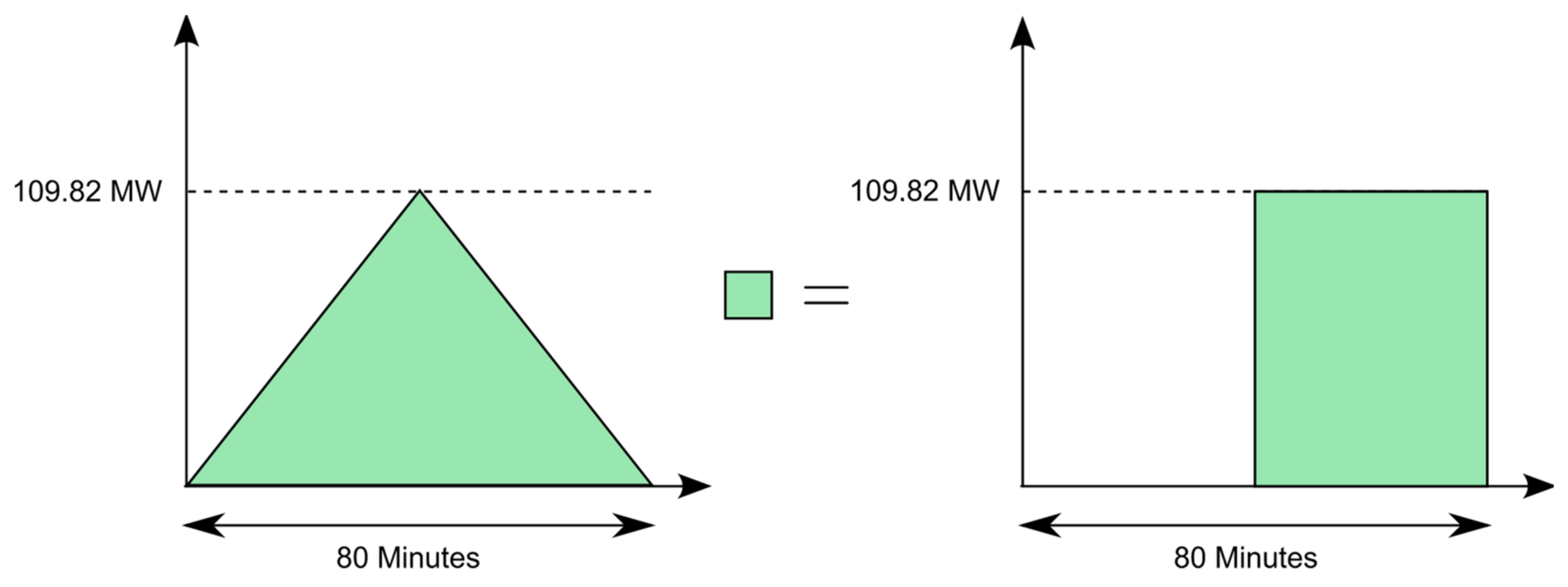In order to supply 1025 MW_thh to the system in 10 h, the system must be charged with a constant charge power of 102.5 MW_th. The integral of the charging power over time corresponds to the thermal energy supplied to the system. During the night, in order to obtain the same thermal energy for the same period of daytime operation, the charge power must be increased. From Figure 6, in the left figure, it can be seen that the difference between a constant power and the consideration of the sunrise and sunset is exactly the thermal energy that would be supplied to the system in 40 min by a constant charging power of 102.5 MW_th. The power must be selected accordingly so that the 1025 MW_thh would be reached in 9 h and 20 min, which leads to the following calculation:

$$\frac{1025 M{W}_{th}h}{9.33 \mathrm{h}}=109.82 M{W}_{th}$$

(1)

The required charging power is thus 109.82 MW_th. This is implemented using the GRADIENT component. This is a dynamic component that limits the rate at which the value of an input signal can change. In this case, the rate for both the increase and the decrease in the input value is limited to 2.75 MW_th min, which can be seen from the following calculation:

$$\frac{109.82 M{W}_{th}h}{40 \min }=2.75\frac{M{W}_{th}}{\min }$$

(2)

The model for heat supply created in APROS can be also seen in Figure 7. This is clearly discussed below:

The setpoint SP01 describes a digital input signal that is sent to a system. In this, the input signal represents the charging power. SP01 and SP05 (the discharging power) are the only variables in the model that must be changed externally during a simulation cycle. All other variables are derived from these or are regulated based on them. SP01 and SP05 are changed by the so-called queue. Queues are around process logs that can be used to influence a system according to a specific schedule. As described above, this input signal first runs through the gradient component and then to the binary switch ASW03. The signal is measured twice between them and sent to other systems as a digital signal. The switch is used in the event that the CST is empty and can no longer be pumped. In this case, the charging power must be set to 0 MW_th immediately, otherwise, the temperature in the model will approach infinity if the mass flow rate decreases. After the binary switch, the signal passes through two gain components. In the first component, the signal is multiplied by a factor of 10⁶ because the following boundary condition is calculated in watts. In the second gain block, the signal is divided by a factor of 3. The charging power is then output via three nodes. The Boundary_Conditions, which convert the digital signal into a heat flow, follow the gain components. Finally, the three heat flows are measured and fed to the heat_pipe in the storage system.

According to [25], the discharge takes 7.5 h. This results in a discharge power of −136.67 MW_th, as shown in the equation (3).

$$\frac{-1025 M{W}_{th}h}{7.5 \mathrm{h}}=-136.66 M{W}_{th}$$

(3)

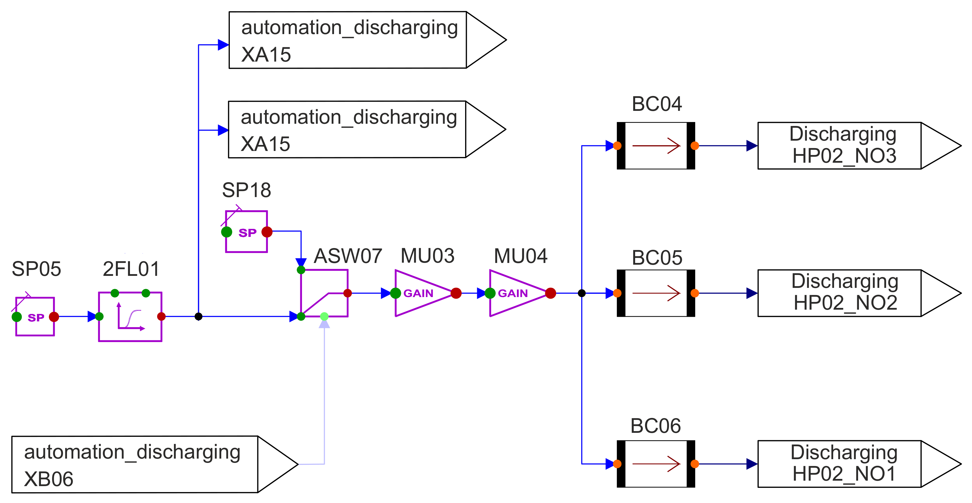
The associated modelling can be seen in Figure 8. This only differs in the input signal and the subsequent component. While a gradient is used for charging to describe sunrise and sunset, only a filter is used for discharging to prevent overheating due to sudden changes in charging power. This means that the heat flow cannot suddenly change to a value of −136.67 MW_th when the input signal changes.

The remaining goals are handled by modifying the regulation and control of the process.

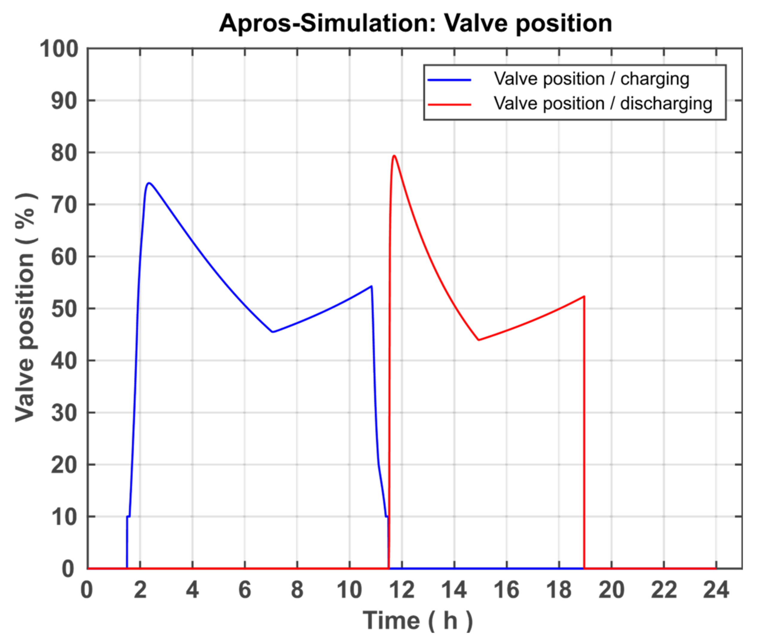
3.1.2. Regulation and Control

Then, the working temperature limits are dealt with at each work step of the real working range of the molten salt. As in the comparison process, this is achieved by regulating the mass flow. The associated APROS automation can be seen in Figure 9 and is explained and described in more detail below:

The temperature at the heat exchanger outlet is measured from the APROS process (Figure 9 top left) and converted into a digital signal with the measurement component TI01. This is compared in the PI controller with the setpoint SP09, which sets a target temperature of 386 °C. A PI controller is used because, according to [19], this is the type of controller commonly used in the industry.

The controller then forwards a signal between 0.1 and 1, which is converted into a valve position between 10% and 100% with the aid of the ACT05 actuator component. A valve position of over 10% is used here to ensure a constant mass flow of >0 kg/s. If the controller has to regulate the mass flow to 0 kg/s in the meantime, nothing will change in the temperature after the heat exchanger, because the heated fluid will not reach the measuring point. The binary_switch ASW01 between the actuator and the PI controller has the function of completely closing the valve if necessary because the PI controller cannot do this due to its working range of 0.1–1 described above. This is needed in two cases. The first case describes the end of the charging process, that is, when no more heat flows into the system. If the measured heat flow (middle left) falls below the value of 0.5, the output signal of the limit-value checker LVC03 changes from true to false. The following OR component then also changes its output signal to false (because one of its input values is false), which leads to the binary_switch jumping to the setpoint SP02 = 0, which results in a valve position of 0%. The second case in which the valve needs to be fully closed occurs when the system is fully charged; this means when the CST falls below 0.65 m level. As shown in Figure 9, this is also modelled using a measured signal and a limit-value checker.

The control of the discharge line is equivalent to that of the charging line, except that the control parameters are adapted to the discharge process (e.g., target temperature = 292 °C).

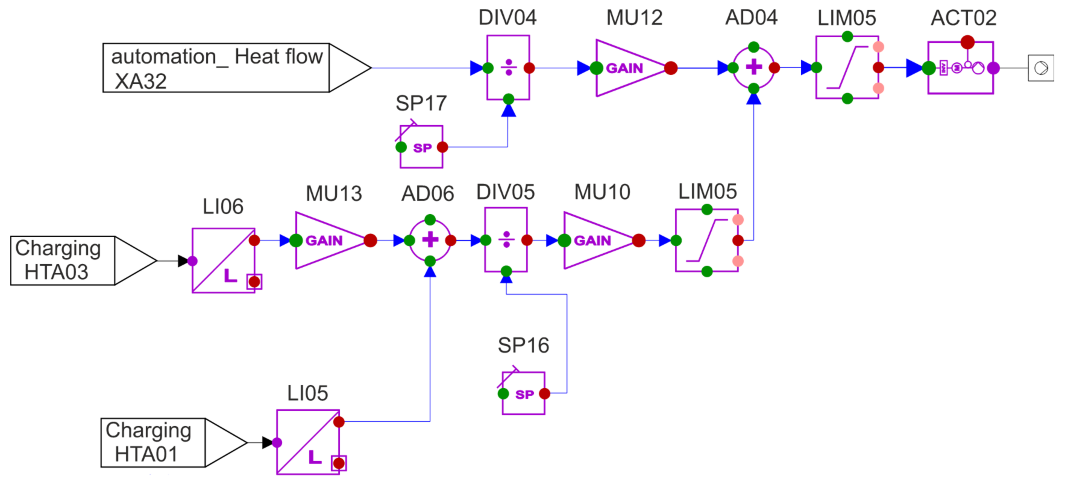
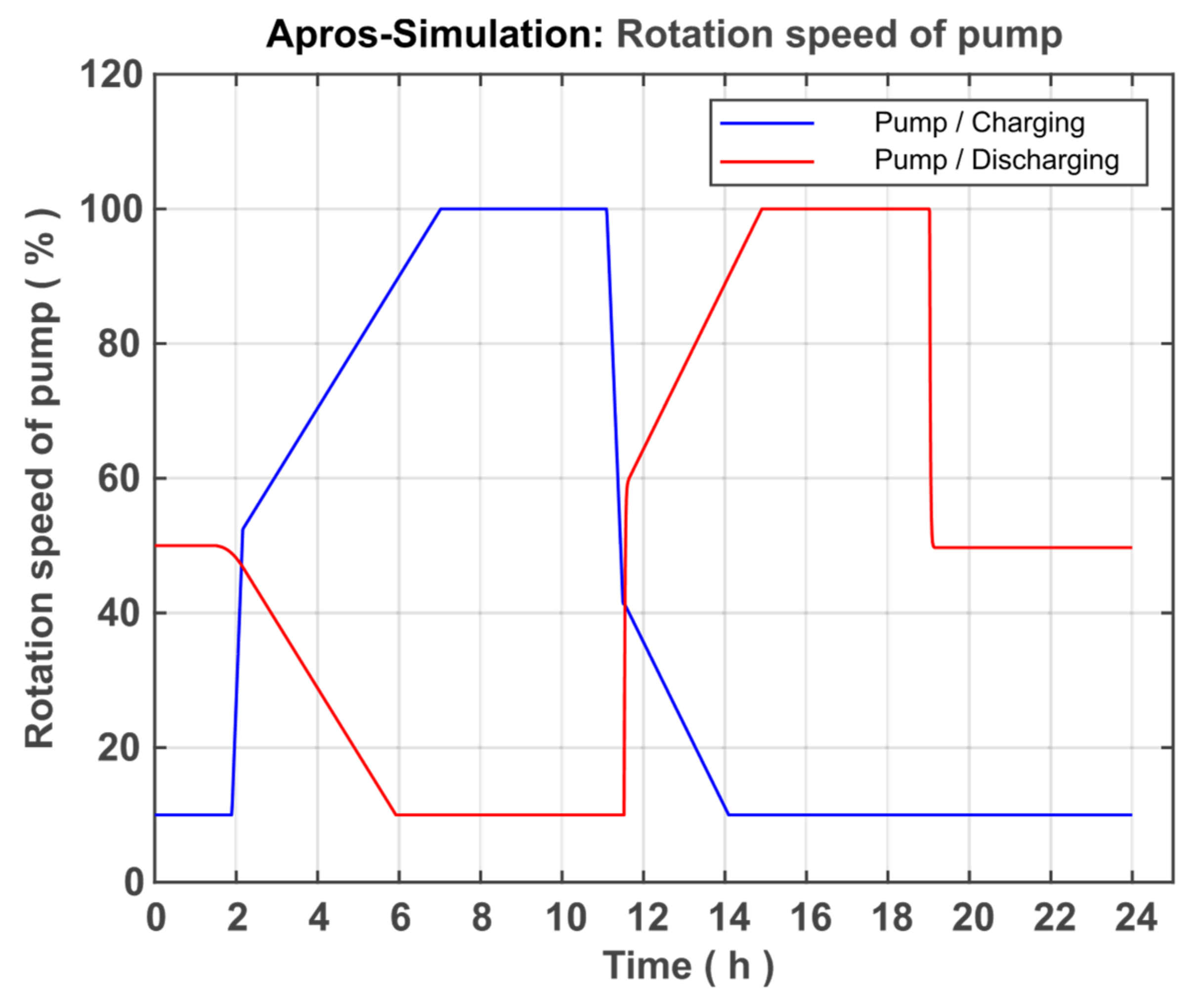
The next step is to try to optimise the pump performance. In the basic model, these pumps ran at 100% performance regardless of the fill level of the tanks and the required mass flow. The reason for this is the associated simplification of the regulation, because the valve regulates continuously at the same pump output and can therefore easily keep the mass flow constant compared to when the pump output changes. However, full power is not always required. For example, when the HST is low, the power required is less than when the level is high. However, it must be ensured here that the pump performance is not directly dependent on the mass flow because this can lead to an interference with the control of mass flow by the valve. As a solution, the pump is controlled based on the charging capacity and the geodetic height difference. The associated APROS automation can be seen in Figure 10 and is described below:

Automation begins with the design principle of the pump to overcome a height difference of 13 m with a capacity of 100% while providing the required mass flow at full discharge capacity. On this basis, the automation shown in Figure 10 calculates the required power and passes it on to the pump via the ACT02 actuator. As described above, two variables are used to determine the power: the geodetic height difference and the charging power. The discharge power is flowed in the upper line, divided by the maximum discharge power (109.83 MW_th) and then multiplied again by a factor of 100. This gives a value showing the percentage of the maximum discharge power currently affecting the system. Between 0 and 50% is deducted from this maximum discharge power by the summation block (AD04) because at full discharge capacity and a geodetic height difference of 13 m (the maximum difference in level between HST and CST), this is slightly more than 50% of the maximum pump capacity. After the summation block (AD04), the signal runs through a limiter, which limits the signal to a range from 10% to 100% in order to always ensure a mass flow >0 kg/s.

The control of the pump in the discharging line is equivalent to the control of the charge line, where 136.67 MW_th of the discharge line is selected as the maximum power.

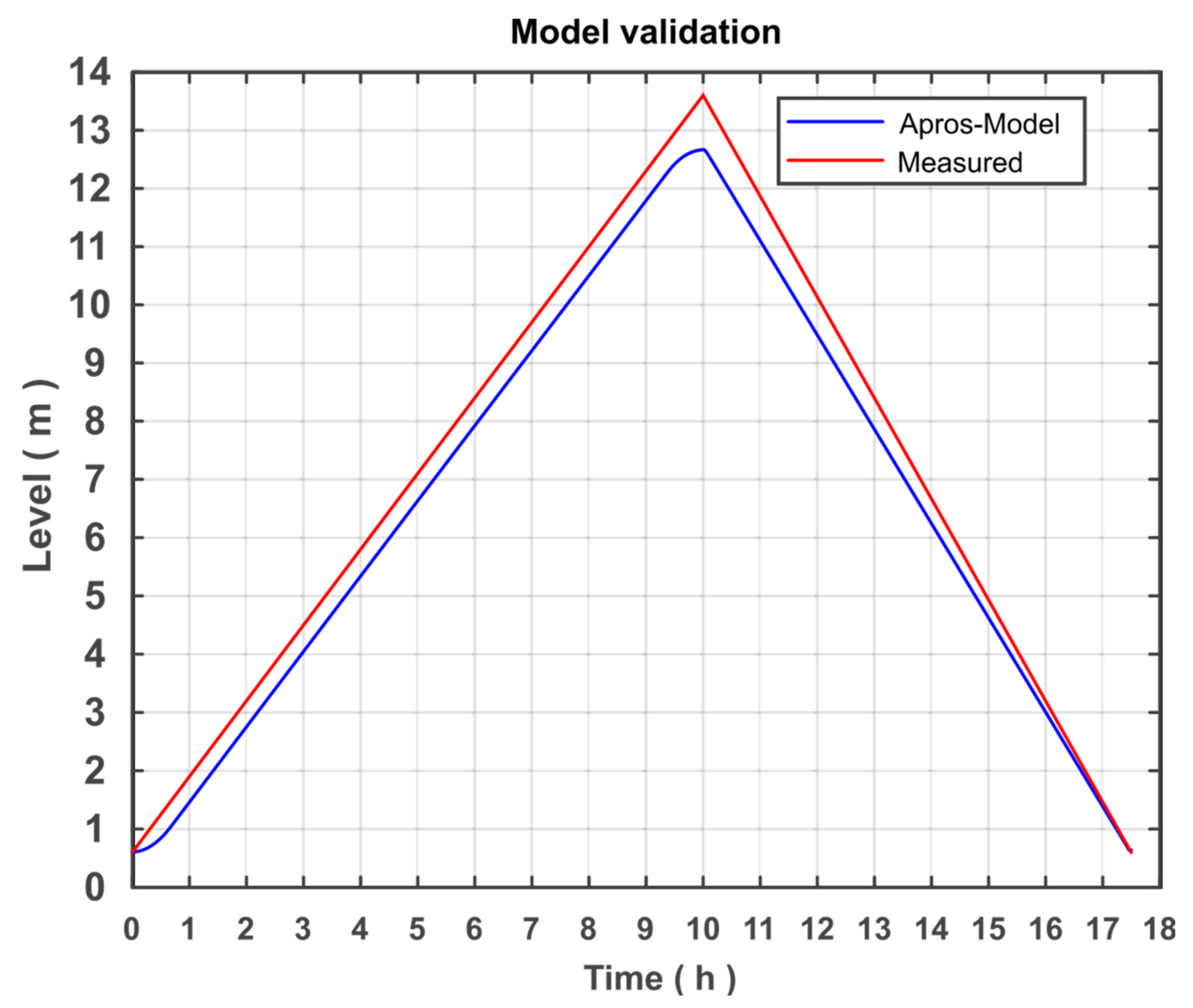
3.2. Model Validation

After the modelling was completed, the model was validated. As described above in Section 3.1, 1025 MW_thh is fed into the system in 10 h and then discharged again in 7.5 h. In the ideal modelling, the CST should be completely filled out after the charging cycle, as in the comparison process of the Andasol 2. Figure 11 shows the level of the comparison process with the APROS model.

The filling level of storage tanks in the APROS model is approximately 12.7 m and in the comparison process is 13.6 m. Accordingly, the deviation of the model is 6.62%, which justifies a confirmation of the system. The error can result from the assumption of an adiabatic change in volume, failure to consider friction, any differences in the physical properties of the modelled liquid salt, or the assumption of an isentropic pump. It should be noted that the error does not come from modelling the sunrise and sunset, as the graph indicates, because the amount of heat supplied is the same.

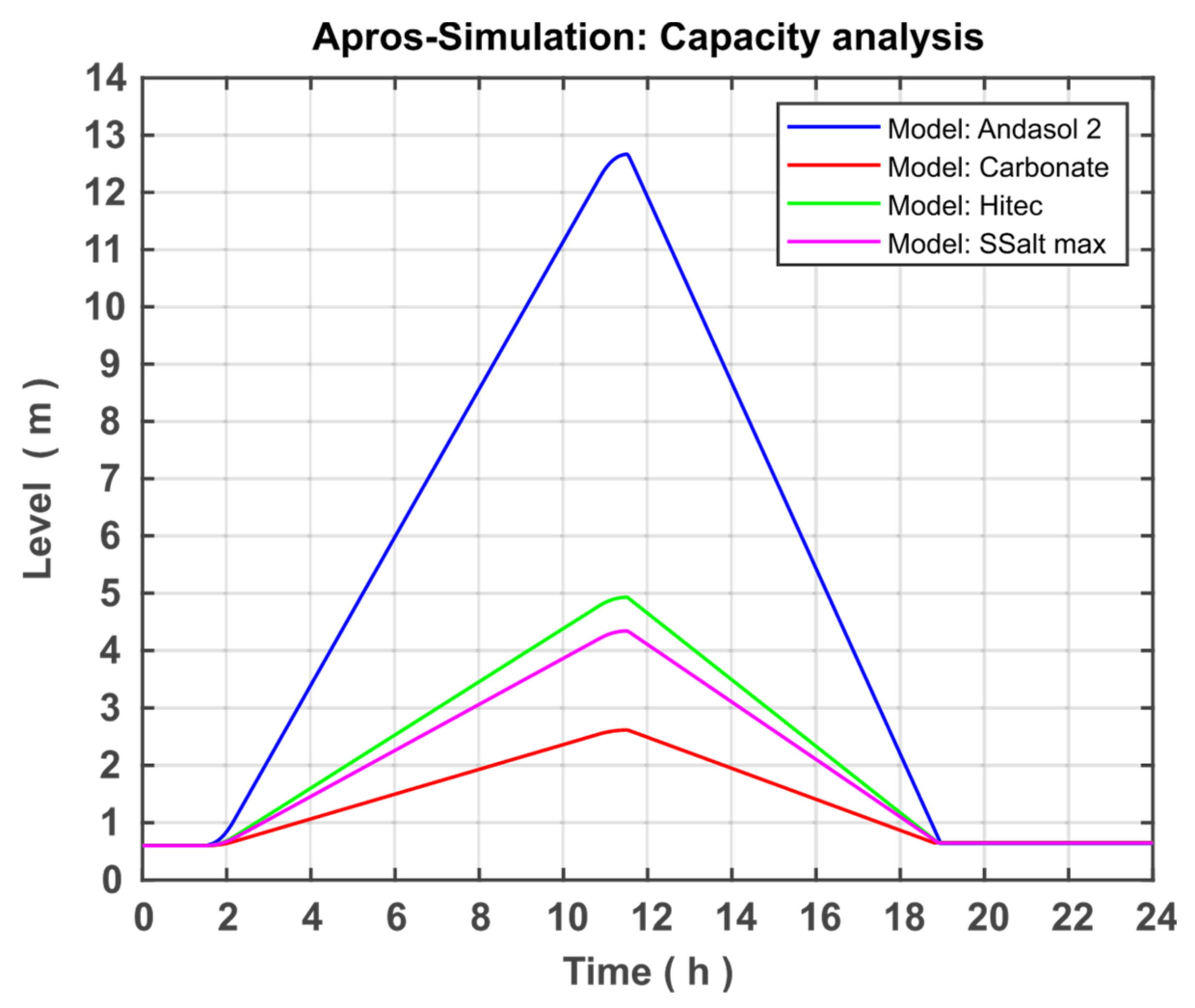
3.3. Design of the Process for Other Storage Fluids

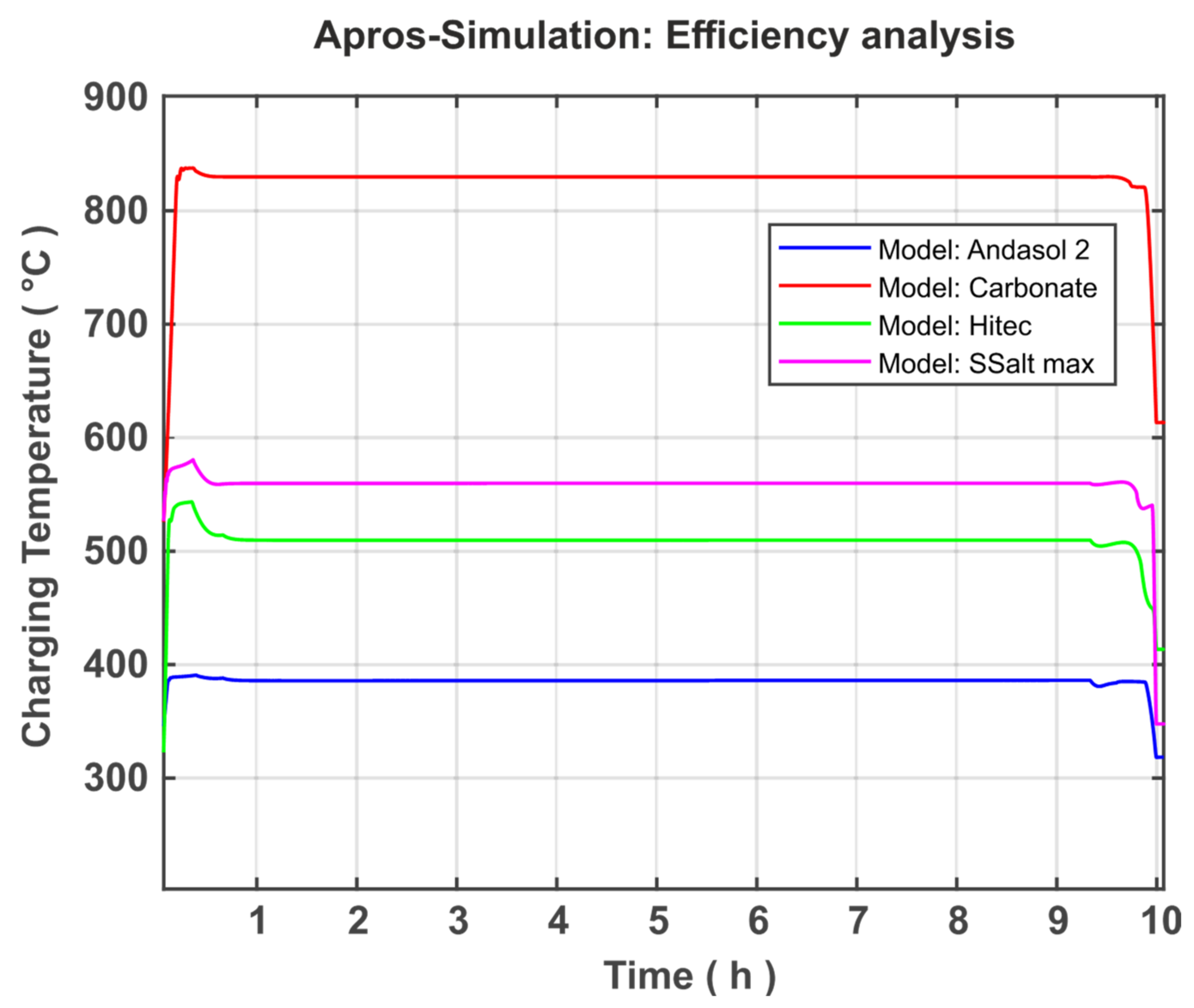
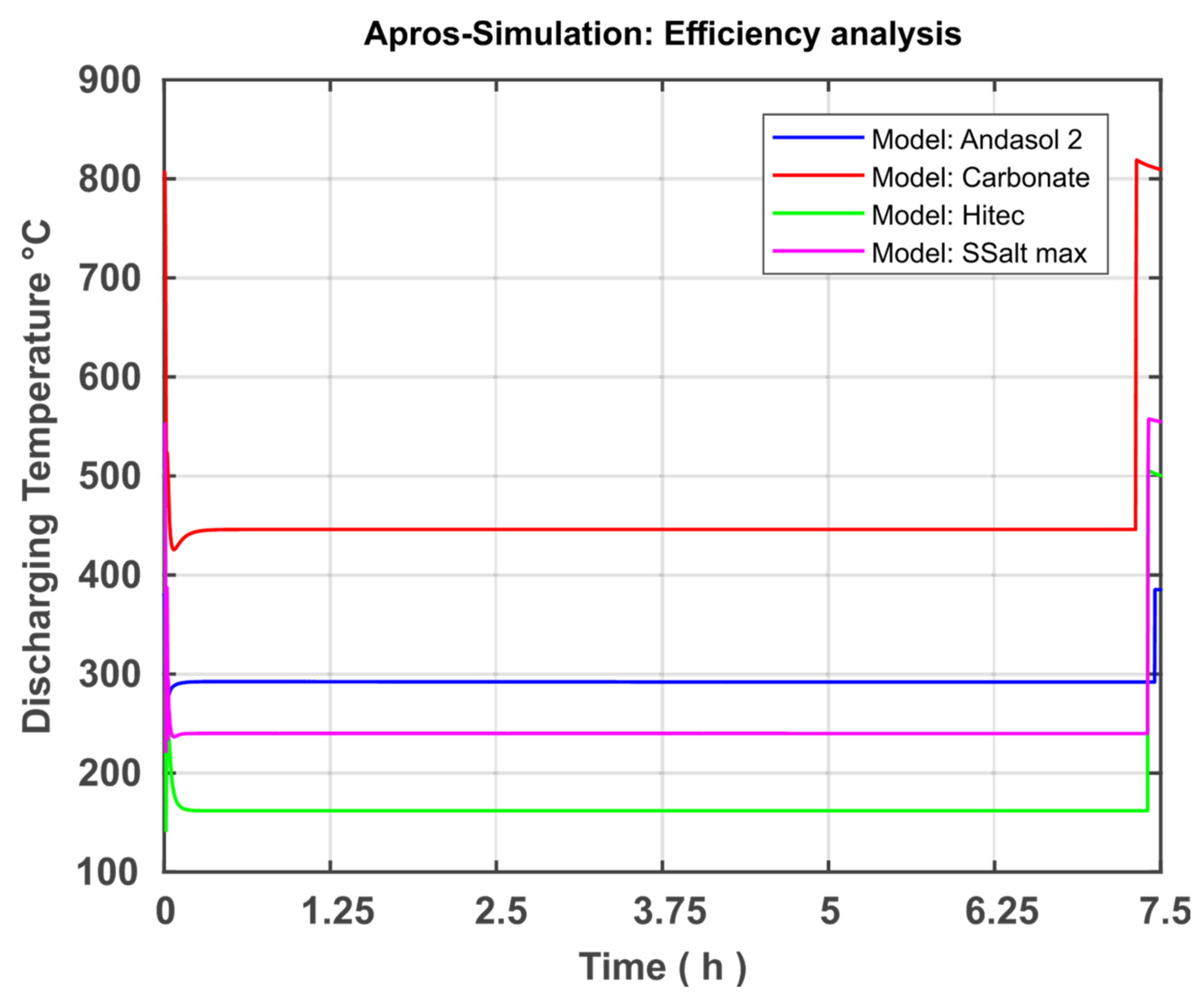
After modelling and model validation are completed, three new models with different storage media or other temperature ranges were created based on the developed model in order to analyse differences and optimisation options. First, the TSS system is operated by the fluid Solar Salt, but the temperature range is extended to the maximum possible range. Because the melting temperature of Solar Salt is 220 °C and the decomposition temperature is 580 °C, the temperature range was set to 240 to 560 °C. The following components must be adapted to the new process requirements: regulation of the mass flows, pump parameters, and valve parameters. The rest of the modelling could be performed.

Second, the Hitec fluid from the APROS database is used. This has a melting temperature of 142 °C and a decomposition temperature of 535 °C. Accordingly, the temperature range is set to 162 to 515 °C. Here, the same components must be adapted as when the working area of the Solar Salt was expanded.

Third, the carbonate salts are used, which have a working temperature higher than nitrate salts. The melting temperature for the carbonate salt specified as optimal in [20] is 400 °C. The decomposition temperature is correspondingly higher (830 °C), which not only promises a greater temperature range than nitrate salt, but also a higher degree of efficiency can be achieved. The specific heat capacity is discussed in the next section in more detail later when implementing carbonate salt in APROS.

Implementation of Carbonate Salt in APROS 6

As the last storage medium, carbonate salt is included in the process so that it can also be compared with the other storage media. Carbonate salt is not one of the predefined fluids that APROS provides, which is why a new fluid must be created in APROS. As described above, the following values are required to define the carbonate salt in APROS: the density, the dynamic viscosity, the specific heat capacity, the thermal conductivity, and the adiabatic compressibility—all depending on the temperature. The selection of the carbonate salt follows the study [20], with the 36 carbonate salts in terms of their usability as a storage medium in sensible heat storage as part of a solar power plant. This identified two suitable carbonate salt compositions: 3% K₂CO₃, 10% Li₂CO₃, 60% Na₂CO₃ and 20% K₂CO₃, 10% Li₂CO₃, 70% Na₂CO₃. The first composition was used in this work because it has a higher decomposition temperature (850 °C). The working temperature range is set to 446 to 830 °C because a distance of 20 degrees from the melting and decomposition point must be maintained. Melting and decomposition points were also taken from [20].

Based on [27], the density of the salt is modelled as a linear function. However, the literature values, which are given in Kelvin, must be converted to degrees Celsius, as APROS only accepts temperatures in Celsius:

$$\rho \left[\mathrm{kg}·{\mathrm{m}}^{-3}\right]=2323-0.4613\times \left(T\right)$$

(4)

In the following, the correlation of the dynamic viscosity is required. This can be found in [28]:

$$\eta \left[\mathrm{mPa}·\mathrm{s}\right]=0.1012\times e^{33400/R·T}$$

(5)

With

$$R \left[\mathrm{J}·{\mathrm{K}}^{-3}·{\mathrm{mol}}^{-3}\right]=8.3143$$

(6)

However, only correlations in the form of polynomials can be inserted into APROS, which is why the formula given in Equation (5) is approximated with a second-degree polynomial for the range from 446 to 830 °C.

A polynomial of the 2nd degree can be formed with these values. The temperature is converted back to Celsius when setting up the polynomial. Thus, the final correlation of the dynamic viscosity and the temperature in degrees Celsius is:

$$\eta \left[\mathrm{Pa}·\mathrm{s}\right]=1.9436\times {10}^{-7}\times T^2-3.0871\times {10}^{-4}\times T+0.126$$

(7)

No studies or other results can be found on the thermal conductivity of carbonate salt. The only evidence about the thermal conductivity λ of such salt can be found in [29]. In that study, the thermal conductivity of LiNO₃, NaNO₃, KNO₃, which is also a carbonate salt and has a similar melting temperature and density, was measured. The thermal conductivity of this salt was determined to be λ = 1.17 W·m⁻¹·°C⁻¹, which is why a thermal conductivity of λ_carb = 1 W·m⁻¹·°C⁻¹ was assumed for the further simulation.

Because the adiabatic compressibility of liquids is negligible, but a value for the compressibility must be assumed in APROS, the value was taken from Solar Salt. Accordingly, the compressibility was set as K_carb = 1.8 × 10⁻⁸ Pa⁻¹. The fluid is now fully defined and could be implemented in APROS.

4. Results

In this section, the results of the various simulations are presented and discussed. First, simulations were carried out with the validated Andasol 2 model and it was checked whether the goals set in the modelling are achieved. The results of the system were also be collected and documented for any weaknesses that may still be present in the model to facilitate further work. The change in the system was then analysed by changing the storage fluid and the temperature range. The associated simulations were compared to each other. Furthermore, the comparison was evaluated based on their storage utilisation and change in efficiency in the thermodynamic cycle. The work cycle of one day (24 h) was used in all simulations.

4.1. System Analysis of the Andasol 2 Model

First, the process values of the Andasol 2 system were analysed and it was determined whether the objectives set in the modelling were achieved. For this purpose, as described above, 24 h were simulated. This was implemented with the help of the full day of the work queue, with which process values and input variables were changed at certain time intervals. The simulation begins at a virtual time of 8:00 a.m. with the loading of the initial conditions (initial condition = 8:00 a.m.) of the process and is thus reset to the initial state, as shown in Figure 11. In this, the mass flow of the two molten salt lines is equal to 0 kg/s, there is no heat flow on the system, the CST is completely filled with a fill level of 13.6 m, and the HST is completely emptied with a fill level of 0.6 m. At 9:30 a.m. the heat flow of the charging line is set to 109.82 MW_th—charging begins. After 10 h the maximum charging capacity of HST is reached. At 19.30 p.m. the charging process is completed and the heat flow is set to 0 MW_th due to the discontinuation of electrical energy from renewable energy sources. Then, the discharging process begins for 7 h and 30 min. For this, the value of the heat flow in the discharge line is set to 136.67 MW_th, which is slowed by the filter after approximately 100 s. At 3:00 a.m. the end of the discharge time is reached and the heat flow of the discharge line is set to 0 MW_th again. From 3:00 a.m. to 8:00 a.m., the system maintains its state without charge or discharge processes, so that at 8:00 a.m., with ideal modelling, the initial conditions should be given again.

In the first step, it is simulated whether the temperature of the molten salt remains within the real working range during the entire process. For this purpose, Figure 12 shows the temperature of the molten salt after the heat exchangers (referred to as heat exchanger in the illustration) in the two charging lines over a 24 h period. As can be seen, the working range of 220 to 580 °C is not exceeded. Furthermore, the set temperature is missed by a maximum of 14 °C (start of discharge) due to the transient behaviour of the control, which corresponds to a maximum control deviation of 4.79%. This means that the goal of delimiting the work area can be classified as achieved. It should be noted that the modelling of sunrise and sunset lengthens the transient process, which can be clearly seen when comparing the two temperature curves. This is an important finding for further simulations and a confirmation of the relevance of modelling the sunrise and sunset. Another relevant finding from the simulation is that the valve after the heat exchanger must be designed for the entire temperature range. As can be seen in the simulation, the valve in the discharge line is only set with a temperature of 292 °C during the discharge period, but it is exposed to the full 386 °C in the rest phase. One explanation for this is that the mass flow of the discharging line is only set to 0 kg/s after the discharge process has ended, so that small amounts of hot fluids can still reach the valve. If an attempt is made to end the discharge process and the mass flow at the same time, a temperature peak occurs shortly before the discharge power and the mass flow are stopped.

In the second step, it is simulated in which area the valves work in the further developed form of the model. The current valve position is plotted as a percentage of the maximum degree of opening. As can be seen in Figure 13, the valves operate in a range of 0–75%, which means that the goal of expanding the control range of the valves has been achieved. This is important for the subsequent construction of the system because with a low degree of opening there are constant flow losses, which further confirms the success of the simulation. It should be noted that an expansion to 0–100% operating range should be a goal. This may be part of further work.

The third simulation shows how the current pump output behaves as a percentage compared to the maximum output during the 24 h. Significant reductions in energy consumption can be achieved here in some sections of the working cycle, as can be seen in Figure 14. It should be noted here, however, that it can be further reduced because the pump in the discharge line is not necessary during the charging period and vice versa. In the simulation shown, however, the performance of the pumps is always >0%, which is why further energy savings are possible. In this way, all of the goals set in the modelling have been achieved, with the possibility of further implementation of these goals as part of the ongoing work.

4.2. System Optimisation

In the following part, the consequences of a change in the temperature range and the storage fluid on the storage tank capacity and the subsequent thermodynamic cycle efficiency should be determined. For this purpose, the three models SSalt max, Hitec, and Carbonate were tested and analysed under the same initial conditions and with the same heat flows as the Andasol 2 model. In detail, all models had the same queue applied to them. The simulation results were then compared with each other and evaluated with regard to a possible increase in storage capacity. In the second part, the individual storage media and working temperatures were evaluated with regard to the resulting change in the efficiency of electricity generation.

4.2.1. Increase in Capacity

Figure 15 shows the respective fill levels of the HST of the four models during a working cycle. As expected, charging the same amount of heat with the SSalt max, Hitec, and Carbonate models leads to a significantly lower fill level than with the Andasol 2 model, because this work used a significantly greater temperature difference, which is presumably with the help of a specific comparable heat capacity, and should be explained using the following formula:

$$Q=m·cp·\left(T_2-T_1\right)$$

(8)

The fill levels of the charging state and the associated increase in storage capacity compared to the Andasol 2 model can be seen in

Table 1. Shows the maximum fill level and increased capacity.

	SSalt Max	Hitec	Carbonate
Fill level max. in m	4.3	4.9	2.61
Increased Capacity in %	295	259	487

.

It must be taken into account that these values are theoretical values that can only be approximated in practice, because, for example, it is only possible with a great deal of effort to design a storage system that approaches the melting and decomposition temperature of the storage medium up to 20 °C as in the simulations. Particularly when carbonate salt is used, the assumption of an adiabatic storage system is associated with a significant error due to the high temperature level, which must be taken into account in practice. Furthermore, the collector principle must be changed regarding system optimisation for the Andasol 2 test facility, because the PT collectors do not allow temperatures above 400 °C due to the mandatory use of thermal oil as HTF.

4.2.2. Increase in Efficiency

When optimising a heat storage system, however, it is not only the capacity increase but also the increase in the efficiency of the thermal power process used to generate electricity in the power plant that must be taken into account, which is associated with an increase in the temperature difference. For this, the theoretically possible thermal efficiency ɳ is calculated by the following formula:

$${\mathsf{ɳ}}_c=1-\frac{T_s}{T_q}$$

(9)

where T_s is the temperature of the heat sink and T_q is the temperature of the heat source.

The temperatures are taken from Figure 16 and Figure 17 to calculate the thermal efficiency. The inflection across the simulation results is deliberately performed in order to check the models for correctness in the same step. This can be confirmed here directly, because all models work with their specified temperature difference. It should be noted that the Hitec model shows a pronounced transient process, which can cause problems in practice. In addition, however, an incorrect design of the controller is also possible.

The comparison shows that the storage medium to be chosen should be carbonate salt, both for increasing efficiency and increasing capacity. With a theoretical increase in efficiency in the thermal power process of up to 18.2%, it exceeds all other storage media and their associated temperature levels.

In addition, the carbonate model has the opportunity to switch two thermodynamic cycle processes one after the other in order to approach the Carnot efficiency [20]. First, a Joule process can be applied to use the temperature range above 600 °C to generate electricity, followed by a steam power cycle, which can use the remainder of the temperature difference. A potential difficulty in the Joule cycle can be found because of the heat exchangers, which must have a high volume due to gas operation. It should be noted here that the consideration of the efficiency is limited to the maximum achievable thermal efficiency, which allows sufficient quantification for a comparison of the processes, but does not provide any information about the real efficiency.

$${\mathsf{ɳ}}_c^{\mathrm{Andasol} 2}=1-\frac{\left(25+273.15\right)K}{\left(386+273.15\right)K}=0.547$$

(10)

$${\mathsf{ɳ}}_c^{\mathrm{Hitec}}=1-\frac{\left(25+273.15\right)K}{\left(515+273.15\right)K}=0.621$$

(11)

$${\mathsf{ɳ}}_c^{\mathrm{SSalt} \max }=1-\frac{\left(25+273.15\right)K}{\left(560+273.15\right)K}=0.642$$

(12)

$${\mathsf{ɳ}}_c^{\mathrm{Carbonate}}=1-\frac{\left(25+273.15\right)K}{\left(830+273.15\right)K}=0.73$$

(13)

During the charging step, an efficiency of 95% was assumed due to heat losses and HTF pump consumption and other requirements (i.e., each 1 MW_el h was converted to 0.95 MW_thh in the molten slat). During the discharging step and according to the previous calculation, the optimal efficiency is 0.73, so that the optimal round-trip efficiency is 0.73 × 0.95 = 0.69. In real cases, the achievable thermal efficiency is lower for a combined cycle power plant. The nominal process efficiency of the combined-cycle power plant (CCPP) can reach 60%. Large-scale combined-cycle power plants with a net electrical power of 780 MW_el and an efficiency level up to 62.2% are now running in Irsching, Germany [30,31], Bouchain, France [32,33], and Tambak Lorok, Indonesia [34,35]. The real round-trip efficiency is expected to 0.62 × 0.95 = 0.589.

5. Conclusions

The present study focused on the creation and further development of a numerical model in APROS for the dynamic system analysis of thermal salt storage facilities. The aim here was the system analysis and optimisation of the thermal salt storage with regard to a stand-alone solution. For this purpose, the theoretical fundamentals were first researched and the properties of power plants and thermal storage systems were explained. In addition, the possibilities of using a TSS in a solar power plant or a stand-alone system were demonstrated. The discussion was extended to the fact that the range of the temperature difference and the storage medium selection is very relevant to TSS optimisation. In the section on modelling and simulation, the development of the model was discussed. The basic model was presented and goals were set for expanding the model. The model was further developed on the basis of these goals. This included the modification of the Andasol 2 comparison system located in Granada, Spain. In the course of this approximation, the created model can be validated by comparing the level of both systems after supplying an identical amount of heat in the same period of time. The discrepancy between both systems was approximately 6.62%, indicating a satisfactory accuracy and allowing the validation of the system. Three additional models were created based on the validated model to analyse the temperature difference and the storage medium. The simulations of the individual models were presented and discussed in the Results section. First, the simulations of the Andasol 2 model were presented. The focus here was on the goals set in the modelling. Both the successful limitation of the working temperature to a technically possible range and the expansion of the valve working range can be recorded. In addition, the pump capacity could be significantly reduced by controlling the pump based on the amount of heat added and the geodetic height difference of the individual storage reservoirs. Then, the four models Andasol 2, SSalt max, Hitec, and Carbonate Salt were evaluated and compared in terms of possible capacity increase and efficiency increase. For the capacity analysis, all models were charged with the same heat quantity as previously and the levels were compared at full fill. The largest increase in capacity of 487% was achieved with the Carbonate Salt model. The greatest increase in efficiency in terms of power generation can also be achieved with the carbonate model (18.2%), whereas the amount of increase was 9.5% and 7.4% for each of SSalt max and Hitec, respectively. With regard to the goal of a stand-alone version, Carbonate Salt can be determined as the optimal storage fluid, as this promises the highest increase in capacity as well as efficiency.

For the stand-alone system, it was found that the charge efficiency is 95%, whereas the discharge efficiency (similar to the existing combined cycle) is 60%. The expected round-trip efficiency of the system is 0.589%, which should be analysed in detail in a future work.