
Wireless Sensor Networks for Enabling Smart Production Lines in Industry 4.0


Abstract
:Featured Application
Abstract
1. Introduction
1.1. Background
1.2. Related Work
1.3. Novelty
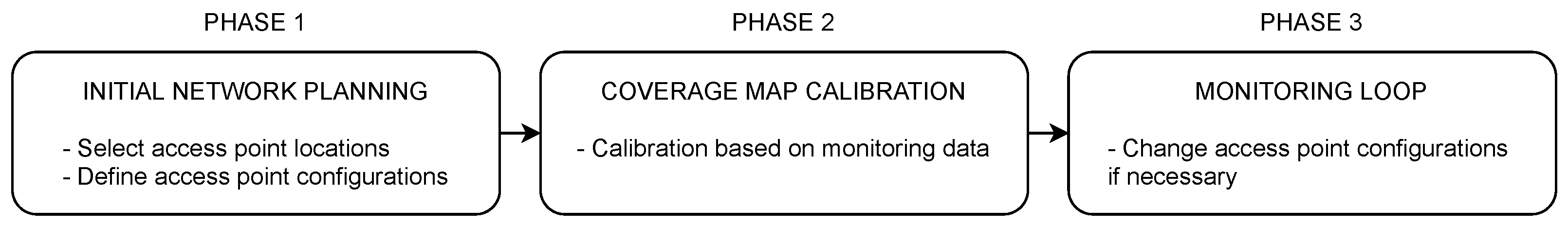
2. Methodology
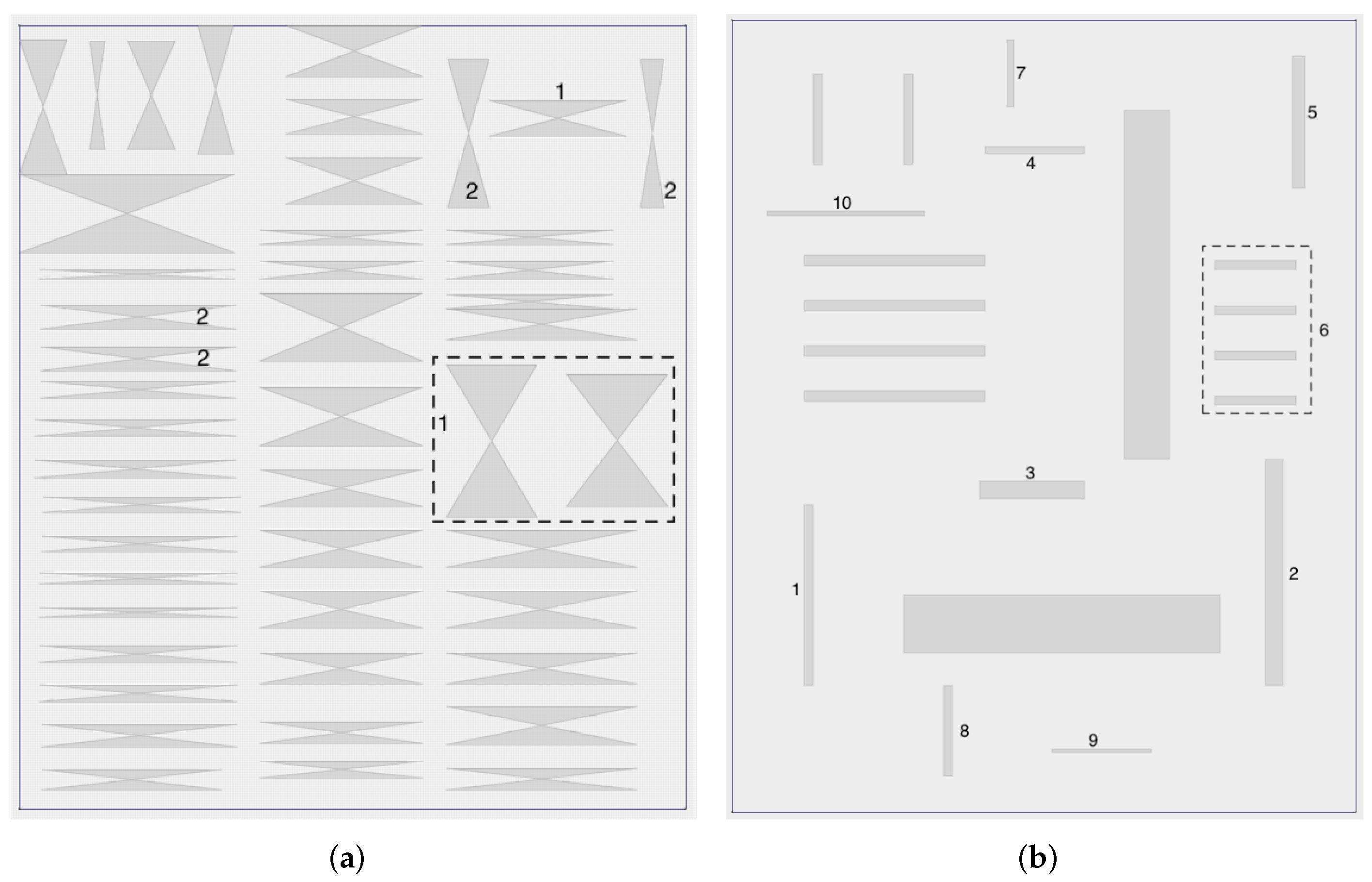
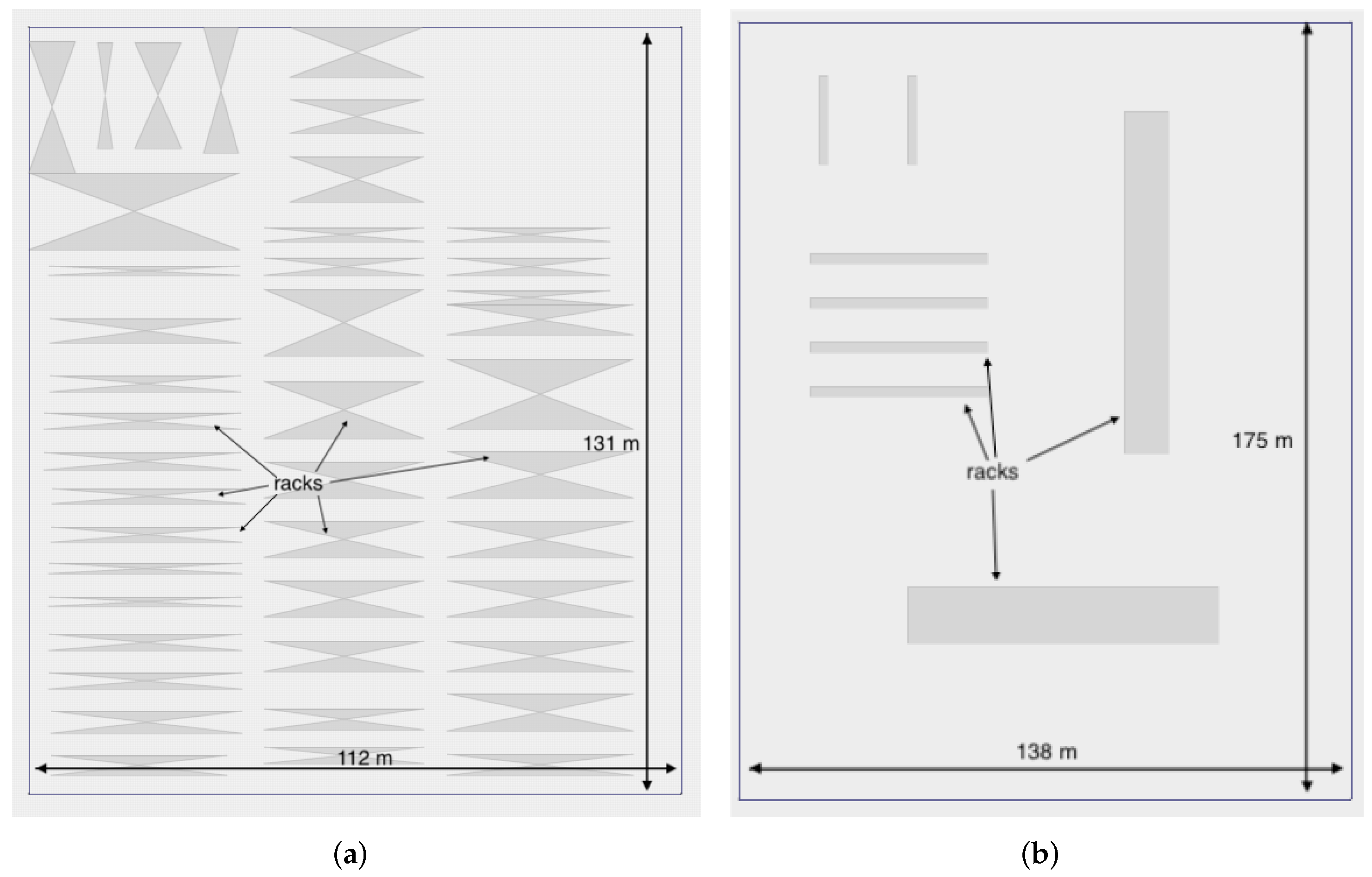
2.1. Considered Environments
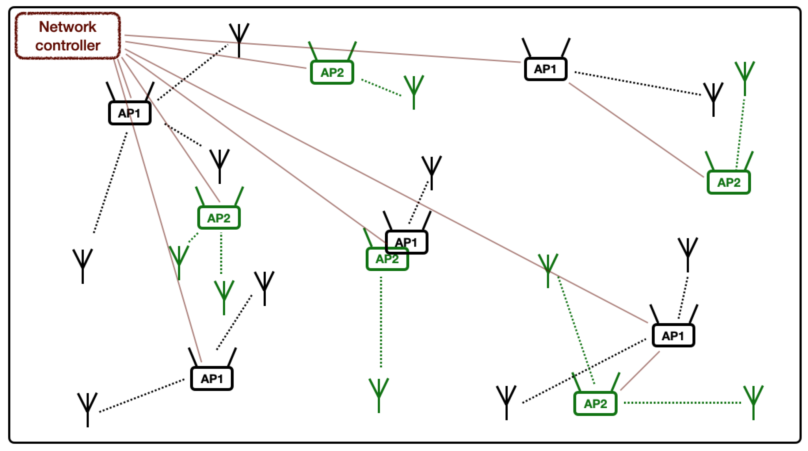
2.2. System Architecture
2.3. Telemetry Data
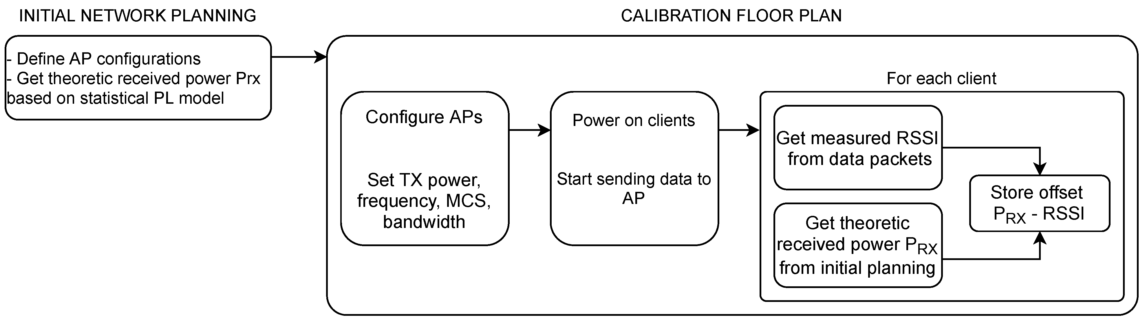
2.4. Initial Physical Layer Network Planning
2.4.1. Coverage and Throughput
2.4.2. Delay and Latency
2.4.3. Other Cost Functions
2.4.4. Hybrid Network Planning
2.5. Coverage Map Calibration
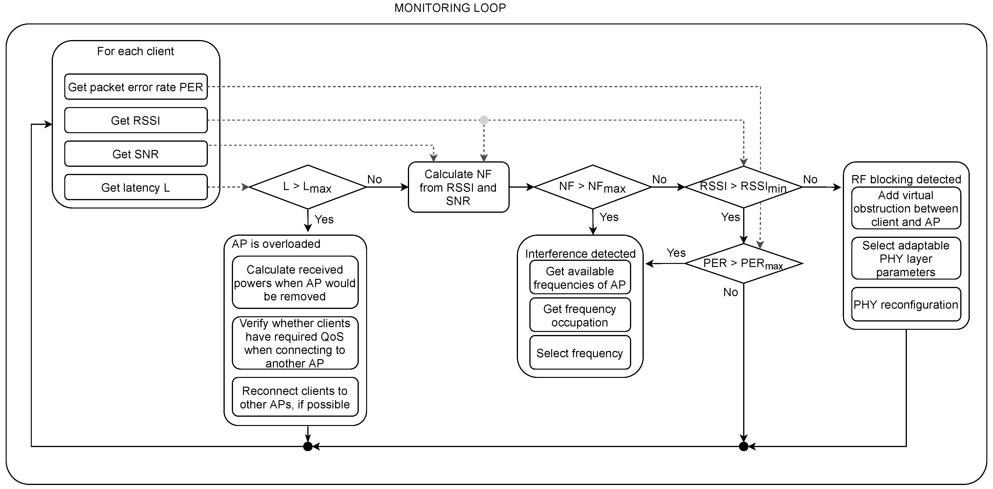
2.6. Closed-Loop Monitoring
3. Algorithm Implementation and Validation via Simulations and Measurements
3.1. Implementation
3.1.1. Overview
3.1.2. Telemetry
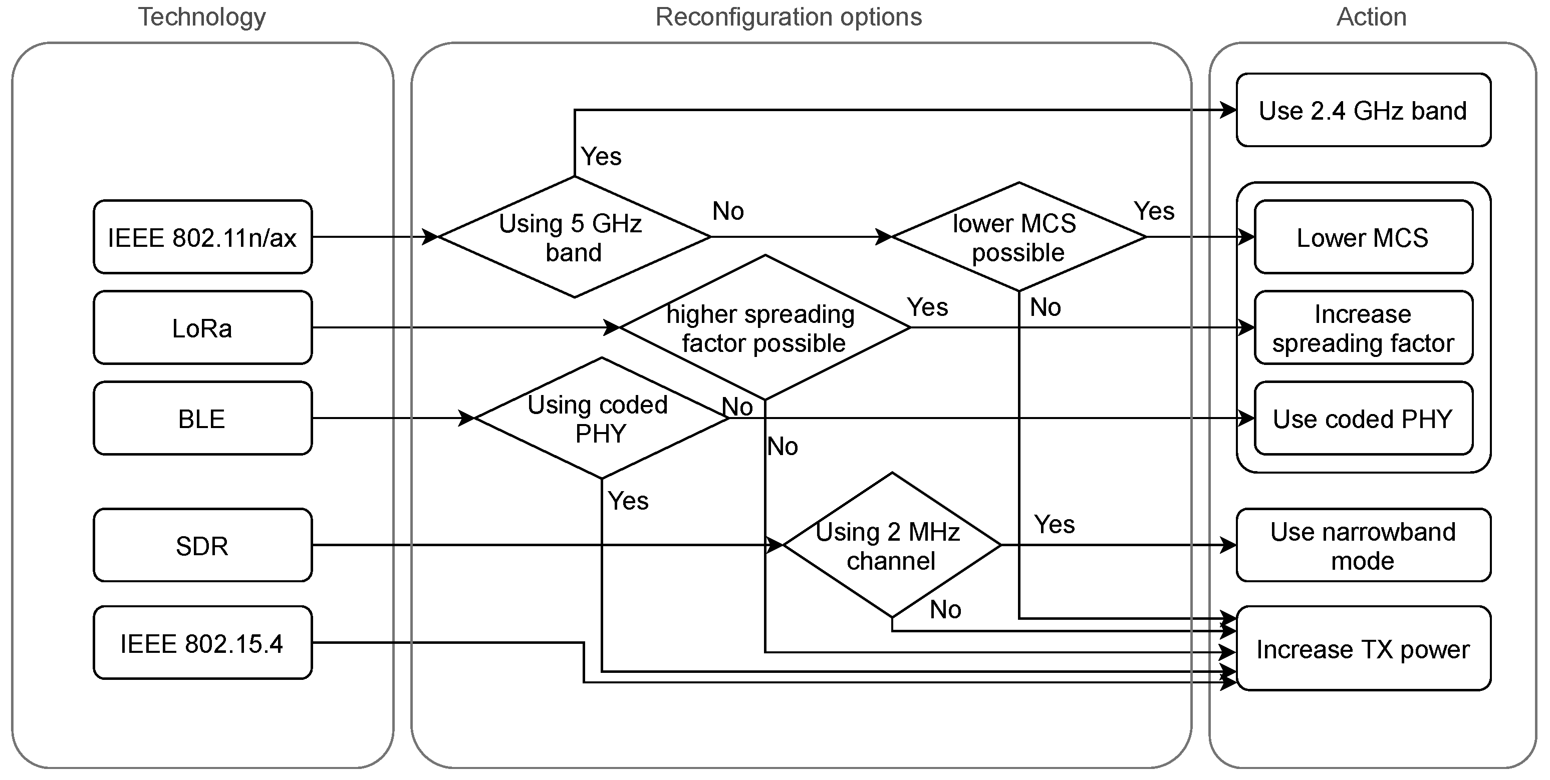
3.1.3. Reconfiguration
3.2. Simulation
3.2.1. Simulation Environment
3.2.2. Simulation Settings
3.3. Validation
3.3.1. Validation Environment
3.3.2. Validation Measurements
4. Results and Discussion
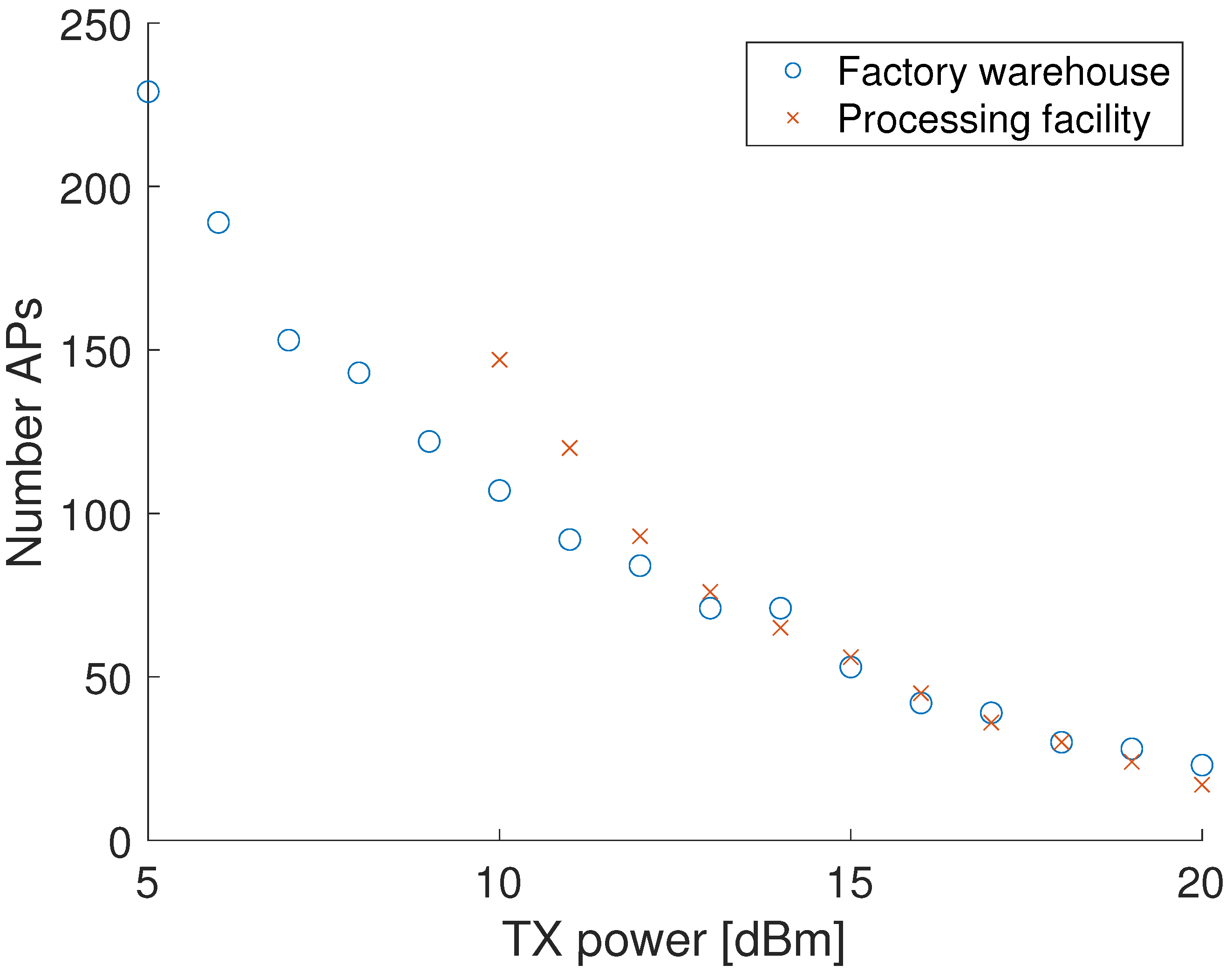
4.1. Initial Network Planning
4.2. Performance Analysis
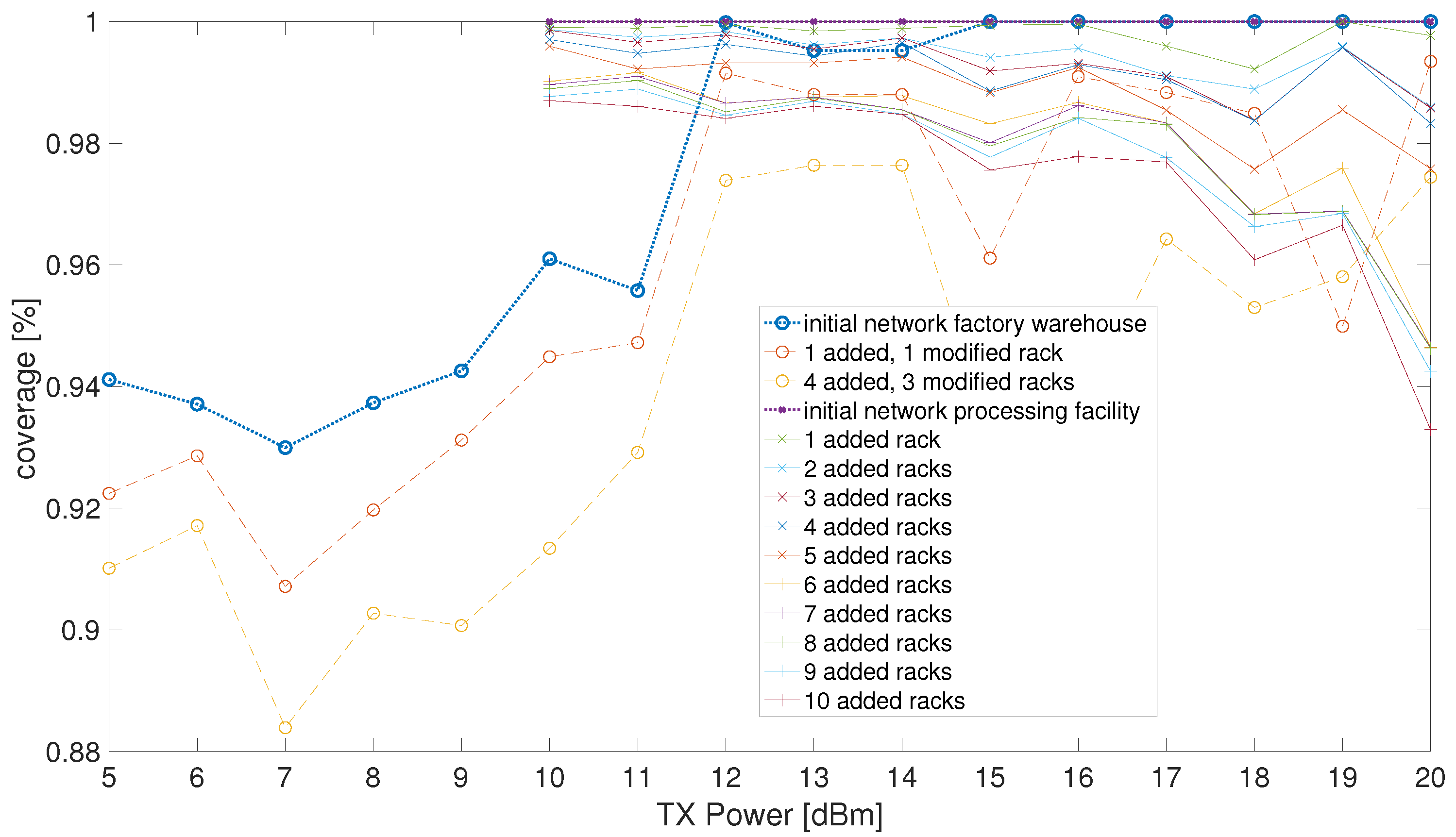
4.2.1. Network Robustness
4.2.2. Network Bandwidth
4.3. Validation in a Real-Time Testbed
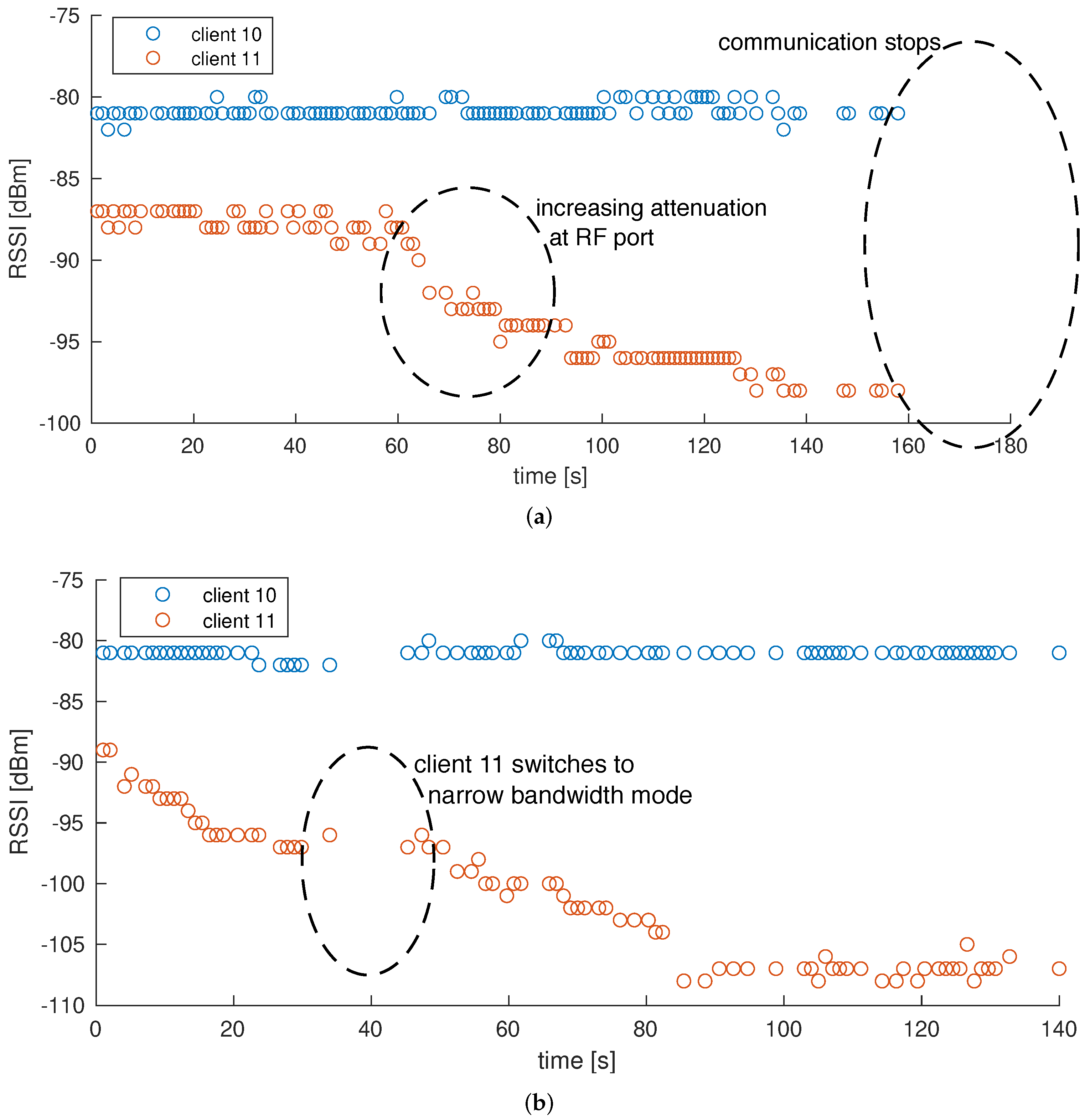
4.3.1. Calibration
4.3.2. Network Reconfiguration
4.4. Comparison to Existing Network-Planning Solutions
5. Conclusions
Author Contributions
Funding
Institutional Review Board Statement
Informed Consent Statement
Data Availability Statement
Acknowledgments
Conflicts of Interest
Abbreviations
| 5G | Fifth Generation |
| AI | Artificial Intelligence |
| AP | Access Point |
| BLE | Bluetooth Low Energy |
| FoF | Factories-of-the-Future |
| I4.0 | Industry 4.0 |
| INT | In-band Network Telemetry |
| IIoT | Industrial Internet of Things |
| ISM | Industrial, Scientific, Medical frequency band |
| LPWAN | Low Power Wide Area Networks |
| MAC | Medium Access Control |
| MCS | Modulation and Coding Scheme |
| MDPI | Multidisciplinary Digital Publishing Institute |
| PHY | Physical layer |
| PoC | Proof-of-concept |
| RF | Radio Frequency |
| SDN | Software Defined Networking |
| SDR | Software Defined Radio |
| PL | Path Loss |
| RF | Radio Frequency |
| QoS | Quality of Service |
| WLAN | Wireless Local Area Network |
| WSN | Wireless Sensor Network |
References
- Oztemel, E.; Gursev, S. Literature review of Industry 4.0 and related technologies. J. Intell. Manuf. 2020, 31, 127–182. [Google Scholar] [CrossRef]
- Adame, T.; Bel, A.; Bellalta, B. Increasing LPWAN Scalability by Means of Concurrent Multiband IoT Technologies: An Industry 4.0 Use Case. IEEE Access 2019, 7, 46990–47010. [Google Scholar] [CrossRef]
- Sherazi, H.H.R.; Grieco, L.A.; Imran, M.A.; Boggia, G. Energy-Efficient LoRaWAN for Industry 4.0 Applications. IEEE Trans. Ind. Inform. 2021, 17, 891–902. [Google Scholar] [CrossRef] [Green Version]
- Wan, J.; Tang, S.; Shu, Z.; Li, D.; Wang, S.; Imran, M.; Vasilakos, A.V. Software-Defined Industrial Internet of Things in the Context of Industry 4.0. IEEE Sens. J. 2016, 16, 7373–7380. [Google Scholar] [CrossRef]
- Mayr, A.; Weigelt, M.; von Lindenfels, J.; Seefried, J.; Ziegler, M.; Mahr, A.; Urban, N.; Kühl, A.; Hüttel, F.; Franke, J. Electric motor production 4.0–application potentials of industry 4.0 technologies in the manufacturing of electric motors. In Proceedings of the 8th International Electric Drives Production Conference (EDPC), Schweinfurt, Germany, 4–5 December 2018; pp. 1–13. [Google Scholar] [CrossRef]
- Cardillo, E.; Caddemi, A. Feasibility study to preserve the health of an industry 4.0 worker: A radar system for monitoring the sitting-time. In Proceedings of the 2019 II Workshop on Metrology for Industry 4.0 and IoT (MetroInd4.0 IoT), Naples, Italy, 4–6 June 2019; pp. 254–258. [Google Scholar] [CrossRef]
- Cerqueira, S.M.; Ferreira da Silva, A.; Santos, C.P. Instrument-based ergonomic assessment: A perspective on the current state of art and future trends. In Proceedings of the 2019 IEEE 6th Portuguese Meeting on Bioengineering (ENBENG), Lisbon, Portugal, 22–23 February 2019; pp. 1–4. [Google Scholar] [CrossRef]
- Dhillon, H.S.; Ganti, R.K.; Baccelli, F.; Andrews, J.G. Modeling and Analysis of K-Tier Downlink Heterogeneous Cellular Networks. IEEE J. Sel. Areas Commun. 2012, 30, 550–560. [Google Scholar] [CrossRef] [Green Version]
- Gong, X.; Plets, D.; Tanghe, E.; De Pessemier, T.; Martens, L.; Joseph, W. An efficient genetic algorithm for large-scale planning of dense and robust industrial wireless networks. Expert Syst. Appl. 2018, 96, 311–329. [Google Scholar] [CrossRef] [Green Version]
- Tanghe, E.; Joseph, W.; Verloock, L.; Martens, L.; Capoen, H.; Herwegen, K.V.; Vantomme, W. The industrial indoor channel: Large-scale and temporal fading at 900, 2400, and 5200 MHz. IEEE Trans. Wirel. Commun. 2008, 7, 2740–2751. [Google Scholar] [CrossRef]
- Aceto, G.; Persico, V.; Pescapé, A. A Survey on Information and Communication Technologies for Industry 4.0: State-of-the-Art, Taxonomies, Perspectives, and Challenges. IEEE Commun. Surv. Tutor. 2019, 21, 3467–3501. [Google Scholar] [CrossRef]
- Mao, S.; Wu, J.; Liu, L.; Lan, D.; Taherkordi, A. Energy-Efficient Cooperative Communication and Computation for Wireless Powered Mobile-Edge Computing. IEEE Syst. J. 2020, 1–12. [Google Scholar] [CrossRef]
- Bajic, B.; Rikalovic, A.; Suzic, N.; Piuri, V. Industry 4.0 Implementation Challenges and Opportunities: A Managerial Perspective. IEEE Syst. J. 2021, 15, 546–559. [Google Scholar] [CrossRef]
- Gokalp, M.O.; Kayabay, K.; Akyol, M.A.; Eren, P.E.; Koçyiğit, A. Big data for industry 4.0: A conceptual framework. In Proceedings of the 2016 International Conference on Computational Science and Computational Intelligence (CSCI), Las Vegas, NV, USA, 15–17 December 2016; pp. 431–434. [Google Scholar] [CrossRef]
- Cemernek, D.; Gursch, H.; Kern, R. Big data as a promoter of industry 4.0: Lessons of the semiconductor industry. In Proceedings of the 2017 IEEE 15th International Conference on Industrial Informatics (INDIN), Emden, Germany, 24–26 July 2017; pp. 239–244. [Google Scholar] [CrossRef]
- Wan, J.; Tang, S.; Li, D.; Imran, M.; Zhang, C.; Liu, C.; Pang, Z. Reconfigurable Smart Factory for Drug Packing in Healthcare Industry 4.0. IEEE Trans. Ind. Inform. 2019, 15, 507–516. [Google Scholar] [CrossRef]
- Caesarendra, W.; Wijaya, T.; Pappachan, B.K.; Tjahjowidodo, T. Adaptation to industry 4.0 using machine learning and cloud computing to improve the conventional method of deburring in aerospace manufacturing industry. In Proceedings of the 2019 12th International Conference on Information Communication Technology and System (ICTS), Surabaya, Indonesia, 18 July 2019; pp. 120–124. [Google Scholar] [CrossRef]
- Prist, M.; Monteriù, A.; Freddi, A.; Cicconi, P.; Giuggioloni, F.; Caizer, E.; Verdini, C.; Longhi, S. Online fault detection: A smart approach for industry 4.0. In Proceedings of the 2020 IEEE International Workshop on Metrology for Industry 4.0 IoT, Rome, Italy, 3–5 June 2020; pp. 167–171. [Google Scholar] [CrossRef]
- Haile, B.B.; Mutafungwa, E.; Hämäläinen, J. A Data-Driven Multiobjective Optimization Framework for Hyperdense 5G network-planning. IEEE Access 2020, 8, 169423–169443. [Google Scholar] [CrossRef]
- Bosio, S.; Capone, A.; Cesana, M. Radio Planning of Wireless Local Area Networks. IEEE/ACM Trans. Netw. 2007, 15, 1414–1427. [Google Scholar] [CrossRef]
- Pramudianto, F.; Simon, J.; Eisenhauer, M.; Khaleel, H.; Pastrone, C.; Spirito, M. Prototyping the internet of things for the future factory using a SOA-based middleware and reliable WSNs. In Proceedings of the 2013 IEEE 18th Conference on Emerging Technologies Factory Automation (ETFA), Cagliari, Italy, 10–13 September 2013; pp. 1–4. [Google Scholar] [CrossRef]
- Khaleel, H.; Penna, F.; Pastrone, C.; Tomasi, R.; Spirito, M.A. Frequency Agile Wireless Sensor Networks: Design and Implementation. IEEE Sens. J. 2012, 12, 1599–1608. [Google Scholar] [CrossRef]
- Mao, S.; Zhang, N.; Liu, L.; Wu, J.; Dong, M.; Ota, K.; Liu, T.; Wu, D. Computation Rate Maximization for Intelligent Reflecting Surface Enhanced Wireless Powered Mobile Edge Computing Networks. IEEE Trans. Veh. Technol. 2021, 70, 10820–10831. [Google Scholar] [CrossRef]
- Govindaraj, K.; Grewe, D.; Artemenko, A.; Kirstaedter, A. Towards zero factory downtime: Edge computing and SDN as enabling technologies. In Proceedings of the 2018 14th International Conference on Wireless and Mobile Computing, Networking and Communications (WiMob), Limassol, Cyprus, 15–17 October 2018; pp. 285–290. [Google Scholar] [CrossRef]
- Lin, S.C.; Wang, P.; Akyildiz, I.F.; Luo, M. Towards Optimal network-planning for Software-Defined Networks. IEEE Trans. Mob. Comput. 2018, 17, 2953–2967. [Google Scholar] [CrossRef]
- Chen, Q.; Zhang, X.J.; Lim, W.L.; Kwok, Y.S.; Sun, S. High Reliability, Low Latency and Cost Effective network-planning for Industrial Wireless Mesh Networks. IEEE/ACM Trans. Netw. 2019, 27, 2354–2362. [Google Scholar] [CrossRef]
- de Melo, P.F.S.; Godoy, E.P. Controller interface for industry 4.0 based on RAMI 4.0 and OPC UA. In Proceedings of the 2019 II Workshop on Metrology for Industry 4.0 and IoT (MetroInd4.0 IoT), Naples, Italy, 4–6 June 2019; pp. 229–234. [Google Scholar] [CrossRef]
- Plets, D.; Joseph, W.; Vanhecke, K.; Tanghe, E.; Martens, L. Coverage Prediction and Optimization Algorithms for Indoor Environments. EURASIP J. Wirel. Commun. Netw. 2012, 2012, 123:1–123:23. [Google Scholar] [CrossRef] [Green Version]
- Plets, D.; Tanghe, E.; Paepens, A.; Martens, L.; Joseph, W. WiFi network-planning and intra-network interference issues in large industrial warehouses. In Proceedings of the 2016 10th European Conference on Antennas and Propagation (EuCAP), Davos, Switzerland, 10–15 April 2016; pp. 1–5. [Google Scholar] [CrossRef] [Green Version]
- Aazam, M.; Zeadally, S.; Harras, K.A. Deploying Fog Computing in Industrial Internet of Things and Industry 4.0. IEEE Trans. Ind. Inform. 2018, 14, 4674–4682. [Google Scholar] [CrossRef]
- Habaebi, M.H.; Nabilah Bt Azizan, N.I. Harvesting WiFi received signal strength indicator (RSSI) for control/automation system in SOHO indoor environment with ESP8266. In Proceedings of the 2016 International Conference on Computer and Communication Engineering (ICCCE), Kuala Lumpur, Malaysi, 26–27 July 2016; pp. 416–421. [Google Scholar] [CrossRef]
- Tan, L.; Su, W.; Zhang, W.; Lv, J.; Zhang, Z.; Miao, J.; Liu, X.; Li, N. In-band Network Telemetry: A Survey. Comput. Netw. 2021, 186, 107763. [Google Scholar] [CrossRef]
- Manzanares-Lopez, P.; Muñoz-Gea, J.P.; Malgosa-Sanahuja, J. Passive In-Band Network Telemetry Systems: The Potential of Programmable Data Plane on Network-Wide Telemetry. IEEE Access 2021, 9, 20391–20409. [Google Scholar] [CrossRef]
- Hyun, J.; Hong, J.W.K. Knowledge-defined networking using in-band network telemetry. In Proceedings of the 2017 19th Asia-Pacific Network Operations and Management Symposium (APNOMS), Seoul, Korea, 27–29 September 2017; pp. 54–57. [Google Scholar] [CrossRef]
- Pan, T.; Song, E.; Bian, Z.; Lin, X.; Peng, X.; Zhang, J.; Huang, T.; Liu, B.; Liu, Y. INT-path: Towards optimal path planning for in-band network-wide telemetry. In Proceedings of the IEEE INFOCOM 2019-IEEE Conference on Computer Communications, Paris, France, 29 April–2 May 2019; pp. 487–495. [Google Scholar] [CrossRef]
- Isolani, P.H.; Haxhibeqiri, J.; Moerman, I.; Hoebeke, J.; Marquez-Barja, J.M.; Granville, L.Z.; Latré, S. An SDN-based framework for slice orchestration using in-band network telemetry in IEEE 802.11. In Proceedings of the 2020 6th IEEE Conference on Network Softwarization (NetSoft), Ghent, Belgium, 29 June–3 July 2020; pp. 344–346. [Google Scholar] [CrossRef]
- Karaagac, A.; De Poorter, E.; Hoebeke, J. In-Band Network Telemetry in Industrial Wireless Sensor Networks. IEEE Trans. Netw. Serv. Manag. 2020, 17, 517–531. [Google Scholar] [CrossRef] [Green Version]
- Doudou, M.; Djenouri, D.; Badache, N. Survey on Latency Issues of Asynchronous MAC Protocols in Delay-Sensitive Wireless Sensor Networks. IEEE Commun. Surv. Tutor. 2013, 15, 528–550. [Google Scholar] [CrossRef]
- Hong, S.H.; Kim, H.K. A multi-hop reservation method for end-to-end latency performance improvement in asynchronous MAC-based wireless sensor networks. IEEE Trans. Consum. Electron. 2009, 55, 1214–1220. [Google Scholar] [CrossRef]
- Yan, H.; Zhang, Y.; Pang, Z.; Xu, L.D. Superframe Planning and Access Latency of Slotted MAC for Industrial WSN in IoT Environment. IEEE Trans. Ind. Inform. 2014, 10, 1242–1251. [Google Scholar] [CrossRef]
- Monica, R.; Davoli, L.; Ferrari, G. A Wave-Based Request-Response Protocol for Latency Minimization in WSNs. IEEE Internet Things J. 2019, 6, 7971–7979. [Google Scholar] [CrossRef]
- Khanafer, M.; Al-Anbagi, I.; Mouftah, H.T. An optimized cluster-based WSN design for latency-critical applications. In Proceedings of the 2017 13th International Wireless Communications and Mobile Computing Conference (IWCMC), Valencia, Spain, 26–30 June 2017; pp. 969–973. [Google Scholar] [CrossRef]
- Shrestha, P.L.; Hempel, M.; Sharif, H.; Chen, H.H. Modeling Latency and Reliability of Hybrid Technology Networking. IEEE Sens. J. 2013, 13, 3616–3624. [Google Scholar] [CrossRef]
- Zafari, F.; Gkelias, A.; Leung, K.K. A Survey of Indoor Localization Systems and Technologies. IEEE Commun. Surv. Tutor. 2019, 21, 2568–2599. [Google Scholar] [CrossRef] [Green Version]
- Liu, H.S.; Pang, G. Positioning beacon system using digital camera and LEDs. IEEE Trans. Veh. Technol. 2003, 52, 406–419. [Google Scholar] [CrossRef] [Green Version]
- Kim, H.S.; Kim, D.R.; Yang, S.H.; Son, Y.H.; Han, S.K. An Indoor Visible Light Communication Positioning System Using a RF Carrier Allocation Technique. J. Light. Technol. 2013, 31, 134–144. [Google Scholar] [CrossRef]
- Yang, S.H.; Jung, E.M.; Han, S.K. Indoor Location Estimation Based on LED Visible Light Communication Using Multiple Optical Receivers. IEEE Commun. Lett. 2013, 17, 1834–1837. [Google Scholar] [CrossRef]
- Luo, J.; Fan, L.; Li, H. Indoor Positioning Systems Based on Visible Light Communication: State of the Art. IEEE Commun. Surv. Tutor. 2017, 19, 2871–2893. [Google Scholar] [CrossRef]
- Zhuang, Y.; Hua, L.; Qi, L.; Yang, J.; Cao, P.; Cao, Y.; Wu, Y.; Thompson, J.; Haas, H. A Survey of Positioning Systems Using Visible LED Lights. IEEE Commun. Surv. Tutor. 2018, 20, 1963–1988. [Google Scholar] [CrossRef] [Green Version]
- Jung, S.Y.; Hann, S.; Park, C.S. TDOA-based optical wireless indoor localization using LED ceiling lamps. IEEE Trans. Consum. Electron. 2011, 57, 1592–1597. [Google Scholar] [CrossRef]
- Paul, A.S.; Wan, E.A. RSSI-Based Indoor Localization and Tracking Using Sigma-Point Kalman Smoothers. IEEE J. Sel. Top. Signal Process. 2009, 3, 860–873. [Google Scholar] [CrossRef]
- Aslam, M.; Jiao, X.; Liu, W.; Moerman, I. An enhanced version of IEEE 802.15.4 standard compliant transceiver supporting variable data rate. In Proceedings of the EuCNC2019, the European Conference on Networks and Communications, Valencia, Spain, 18–21 June 2019; p. 2. [Google Scholar]
- Kohler, E.; Morris, R.; Chen, B.; Jannotti, J.; Kaashoek, M.F. The Click Modular Router. ACM Trans. Comput. Syst. 2000, 18, 263–297. [Google Scholar] [CrossRef]
- Haxhibeqiri, J.; Moerman, I.; Hoebeke, J. Low overhead, fine-grained end-to-end monitoring of wireless networks using in-band telemetry. In Proceedings of the 2019 15th International Conference on Network and Service Management (CNSM), Halifax, NS, Canada, 21–25 October 2019; pp. 1–5. [Google Scholar] [CrossRef] [Green Version]
- IEEE Standard for Low-Rate Wireless Networks-Redline. IEEE Std 802.15.4-2020 (Revision of IEEE Std 802.15.4-2015)-Redline; IEEE: Piscataway, NJ, USA, 2020; pp. 1–1294. [Google Scholar]


| Parameter | Standard BW Mode | Narrow BW Mode |
|---|---|---|
| Bandwidth (MHz) | 2 | 0.25 |
| Data rate (kbps) | 250 | 31.25 |
| Sensitivity (dBm) | −98 | −107 |
| Technology | Transmit Power | Frequency | MCS | Bandwidth |
|---|---|---|---|---|
| IEEE 802.11n/ax | ✓ | ✓ | ✓ | |
| LoRa | ✓ | ✓ | ||
| BLE | ✓ | ✓ | ||
| SDR IEEE 802.15.4 | ✓ | ✓ | ✓ | |
| standard IEEE 802.15.4 | ✓ | ✓ |
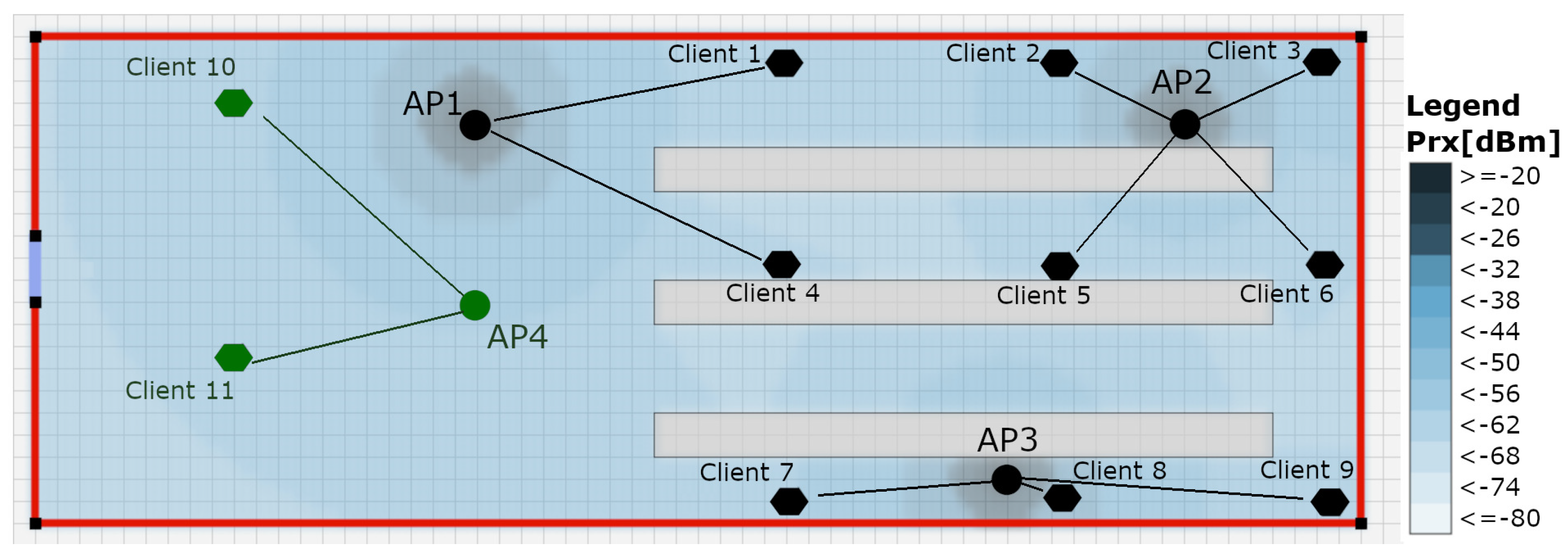
| Client | 1 | 2 | 3 | 4 | 5 | 6 | 7 | 8 | 9 | 10 | 11 |
|---|---|---|---|---|---|---|---|---|---|---|---|
| theoretic | −48 | −41 | −42 | −51 | −49 | −49 | −45 | −34 | −48 | −65 | −63 |
| measured RSSI | −56 | −50 | −48 | −57 | −48 | −32 | −36 | −43 | −47 | −82 | −87 |
Publisher’s Note: MDPI stays neutral with regard to jurisdictional claims in published maps and institutional affiliations. |
© 2021 by the authors. Licensee MDPI, Basel, Switzerland. This article is an open access article distributed under the terms and conditions of the Creative Commons Attribution (CC BY) license (https://creativecommons.org/licenses/by/4.0/).
Share and Cite
De Beelde, B.; Plets, D.; Joseph, W. Wireless Sensor Networks for Enabling Smart Production Lines in Industry 4.0. Appl. Sci. 2021, 11, 11248. https://doi.org/10.3390/app112311248
De Beelde B, Plets D, Joseph W. Wireless Sensor Networks for Enabling Smart Production Lines in Industry 4.0. Applied Sciences. 2021; 11(23):11248. https://doi.org/10.3390/app112311248
Chicago/Turabian StyleDe Beelde, Brecht, David Plets, and Wout Joseph. 2021. "Wireless Sensor Networks for Enabling Smart Production Lines in Industry 4.0" Applied Sciences 11, no. 23: 11248. https://doi.org/10.3390/app112311248
APA StyleDe Beelde, B., Plets, D., & Joseph, W. (2021). Wireless Sensor Networks for Enabling Smart Production Lines in Industry 4.0. Applied Sciences, 11(23), 11248. https://doi.org/10.3390/app112311248