Article

Lagrangian Data Assimilation for Improving Model Estimates of Velocity Fields and Residual Currents in a Tidal Estuary

1
Civil and Environmental Engineering, University of the Sunshine Coast, Sunshine Coast, QLD 4556, Australia
2
Environmental Fluid Mechanics Group, Queensland University of Technology, Brisbane, QLD 4000, Australia
3
BMT, 20 Parkland Rd, Osborne Park, Perth, WA 6017, Australia
4
Sustainability Research Centre, University of the Sunshine Coast, Sunshine Coast, QLD 4556, Australia
5
Mountain Societies Research Institute, University of Central Asia, Khorog 736000, Tajikistan
*
Author to whom correspondence should be addressed.
Appl. Sci. 2021, 11(22), 11006; https://doi.org/10.3390/app112211006
Submission received: 19 October 2021 / Revised: 11 November 2021 / Accepted: 16 November 2021 / Published: 20 November 2021
(This article belongs to the Special Issue Maritime Hydraulics: Analysis and Modeling)

Abstract

:
Numerical models are associated with uncertainties that can be reduced through data assimilation (DA). Lower costs have driven a recent tendency to use Lagrangian instruments such as drifters and floats to obtain information about water bodies. However, difficulties emerge in their assimilation, since Lagrangian data are set out in a moving frame of reference and are not compatible with the fixed grid locations used in models to predict flow variables. We applied a pseudo-Lagrangian approach using OpenDA, an open-source DA tool to assimilate Lagrangian drifter data into an estuarine hydrodynamic model. Despite inherent challenges with using drifter datasets, the work showed that low-cost, low-resolution drifters can provide a relatively higher improvement over the Eulerian dataset due to the larger area coverage of the drifter. We showed that the assimilation of Lagrangian data obtained from GPS-tracked drifters in a tidal channel for a few hours can significantly improve modelled velocity fields (up to 30% herein). A 40% improvement in residual current direction was obtained when assimilating both Lagrangian and Eulerian data. We conclude that the best results are achieved when both Lagrangian and Eulerian datasets are assimilated into the hydrodynamic model.

1. Introduction

A considerable proportion of estuaries have intermittently open connections to the ocean, presenting the typical characteristics of Intermittently Closed and Open Lakes and Lagoons (ICOLLs) [1]. Natural and anthropogenic hazards such as climate change, growing human populations and increasing urbanisation produce many pressures on estuaries and have a negative impact on human assets and livelihoods [2,3].
Consistent with effectively managing estuarine systems, monitoring methods have received attention due to advances in the realism of numerical models, which facilitates high-resolution simulations of such systems. This monitoring requires two types of information: (1) a numerical model that describes the hydrodynamics of the system and (2) measurements used for model simulation that incorporates a more comprehensive mechanism (i.e., a data assimilation (DA) scheme) to improve model estimates. In response to decision makers’ requirements to identify the extent of estuarine problems, reliably measured data are essential to understand system characteristics via numerical modelling. Evolution in technologies has led to more extensive and accurate observational datasets, which have substantially improved the ability to examine model performance [4].
Because observations are approximations to the truth, a befitting combination of observations and theory is required to replicate the truth as much as is achievable [5]. Although Gauss was addressing planetary orbits, his declaration also extends to our circumstances. DA is a process through which a model of a dynamic system is improved by incorporating observations of the real system to make a suitable combination of observations and theory [6].
Measured data alone are often insufficient to provide adequate insight into the physics of the system to support high-quality decision-making in management planning, particularly with regard to complex waterbodies like estuaries. Due to cost and technical limitations, field experiments are often restricted to fixed locations and within certain periods of time. Additionally, observation errors and anomalies can result in the misunderstanding of real physical processes, highlighting the importance of merging numerical modelling with observations to provide valuable flow behaviour information. DA is an effective tool that allows us to combine mathematical models, data resulting from instrumental measurements and prior information for the analysis of complex physical phenomena [7].
Estuarine hydrodynamics are traditionally studied using Eulerian measurements using fixed-position instruments; these sparse and discrete data have also been used to estimate boundary conditions of numerical models, in addition to model calibration and validation [8]. In response to the gap in data density and continuity and in view of these constraints, Lagrangian drifters (i.e., moving sensors) have recently been introduced for estuarine applications [9,10]. The most commonly in situ instruments used for measuring currents are the Acoustic Doppler Current Profiler (ADCP), acoustic doppler velocimeter (ADV) and conductivity–temperature–depth (CTD) profiler [11,12], which can be deployed as a fixed-point instrument (anchored). These instruments measure only the temporal variation of the currents at a certain depth and location; thus, the small control volume of Eulerian devices, including their inability to sample the spatial structure of large domains, necessitates the application of a large number of instruments [13].
Lagrangian drifters have been extensively used in oceanic systems [14], largely because they provide deeper insights into flow dynamics as they carry multiple physical, chemical, or environmental information of the flow and are more cost-effective than Eulerian measurements [15]. Lagrangian DA substantially improves the accuracy of modelled velocity fields of large water systems and are more effective than fixed-measurements DA in improving oceanic circulation models, especially with limited instrumentation [16]. Some studies have also indicated that Lagrangian DA can significantly improve model estimates for small-scale water systems, e.g., rivers [4,15,17]; however, the application of these data in shallow estuaries and inland waters is in its infancy up to this time.
Despite the value of using Lagrangian drifters to study the hydrodynamics of estuaries, particularly where fixed sensor availability is limited, there are some major challenges linked to using these data. Lagrangian drifter motions can be affected by local perturbations due to physical processes, such as wind-induced currents and turbulence, and they are restricted to the free water surface [18]. Because these small-scale features cannot be effectively resolved in hydrodynamic models, data pre-processing is essential prior to DA [15]. In addition, a key facet of the Lagrangian DA process is the difference between the observational (Lagrangian) and numerical model (Eulerian) frameworks; this requires extracting Eulerian velocity from Lagrangian data [16].
Methods introduced for DA fall into two general categories: (i) variational methods, including 3D-VAR and 4D-VAR; (ii) sequential methods, including Kalman filtering and its variants and particle filtering. Sequential methods are robust techniques for DA in a broad range of applications [19]. Different DA schemes have been used to assimilate Lagrangian data into hydrodynamic models; among them, the Ensemble Kalman Filter (EnKF) algorithms are gaining more attention in water systems due to ease of implementation in addition to applicability for non-linear systems [16,19,20]. Using the EnKF algorithm, we can assess the effects of several elements, including the number of ensembles, frequency of assimilation, and observation density (number of drifters), to obtain an effective DA system [21].
The two main reasons that constrain the application of Lagrangian DA in estuarine dynamics studies are the programming effort required and the underestimation of the value of such assimilation. Herein, we present a flexible and easy-to-implement framework in which we use OpenDA; an open-source DA software for Lagrangian data assimilation. OpenDA has been widely used for DA and calibration purposes in lakes, rivers, and estuaries; however, cost-effective GPS-tracked Lagrangian drifters have not previously been used in an estuary.
Sediment transport processes in tidal channels usually result in erosion and deposition [22]. Determination of water circulation patterns in estuaries is a key element to support the sustainable management of these systems [23]. Tidal systems with asymmetric flow properties induce residual currents that cause net flow migration in either the ebb or flood direction [24]. It is also evident that, in tidal systems, residual currents are dominant in one direction; opposite residual currents can occur locally and change the direction of flow [25]. Residual currents control the exchange of sediments, including adsorbed nutrients and contaminants with the adjacent coastal zones and consequently impact geomorphic processes (e.g., stream meandering, bank erosion) and the overall health of estuarine ecosystems. The direction of residual currents (non-tidal currents) is important in sediment transport and bank erosion studies in estuaries because residual circulation and flood/ebb tidal asymmetry are the major mechanisms controlling the transport of fine suspended sediment [26]. In Currimundi Lake, with an asymmetric behaviour, in addition to the longshore transport of sand resulting in the migration of the inlet channel, the net flow direction has a pivotal impact on sand redirection causing bank erosion and entrance channel migration. Thus, tidal hydrodynamics and entrance behaviour studies of the lake play a key role in the effective management of the problems that this estuary encounters.
In this paper, we focused on the application of an EnKF to examine the reliability of Lagrangian DA performance using cost-effective drifters to improve velocity and direction of residual current estimates in Currimundi Lake. Our aim was to: (i) investigate the performance of Lagrangian DA, for improving the accuracy of model predictions; (ii) reduce the programming effort required for assimilation of Lagrangian data into hydrodynamic models; (iii) examine the effect of Eulerian and Eulerian–Lagrangian assimilation on DA performance; and (iv) investigate the spatial variation of residual currents in the domain through identifying five model scenarios increasing the modelling time window from 21 h to 8 days.
Delft3D flexible mesh in 2D mode was used for hydrodynamic simulations for five different time windows (i.e., 21 h, one day, two days, four days, and eight days). We then calculated Eulerian velocities from Lagrangian positions using a pseudo-Lagrangian approach and assimilated Lagrangian velocities using the EnKF method, embodied in OpenDA. In the next step, we conducted an extensive study to quantify the efficiency of EnKF–Lagrangian data assimilation as a function of the number of ensembles, the frequency of assimilation, and the number of drifters, taking into account the uncertainties associated with the boundary forcing of the model and observations. The performance of the Lagrangian assimilation was also compared with Eulerian data assimilation (i.e., fixed-point velocities), along with assimilating both Lagrangian and Eulerian velocities. To examine the effect of DA on the residual velocity direction in the lake, we quantified the variation of residual velocity direction in a situation when the model time window increased while a constant assimilation window was adopted.
The paper is organised as follows: in Section 2, we describe the materials and methods; in Section 3, we provide a brief introduction to the DA environment (OpenDA) and its EnKF module and DA set up, along with describing a post-processing method to remove fluctuations from drifter data. The DA experiments and monitoring network used to investigate the DA performance are presented in Section 4, followed by results and discussion in Section 5. Finally, we present a detailed summary of the study and the conclusions from the simulation results in Section 6.

2. Materials and Methods
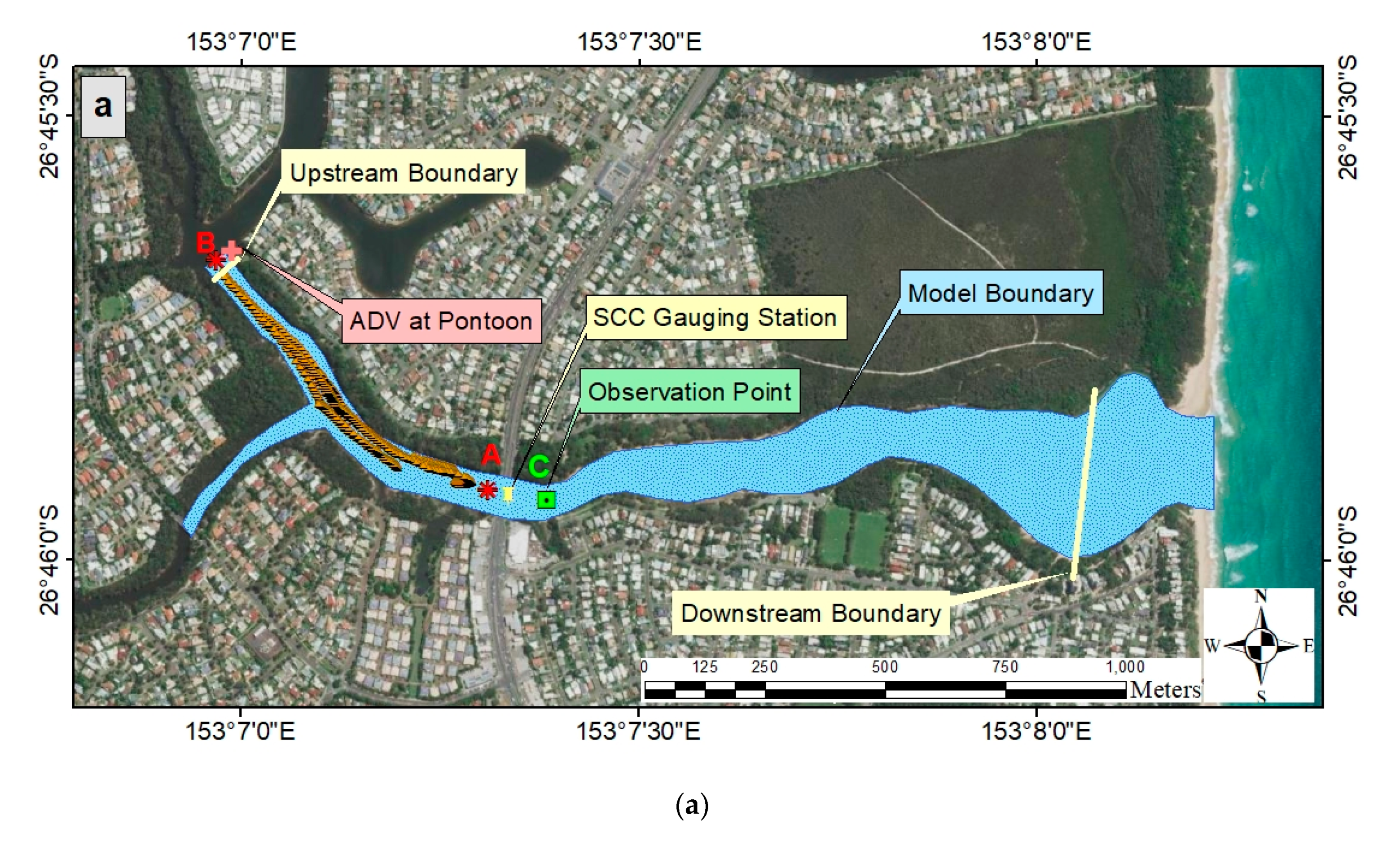
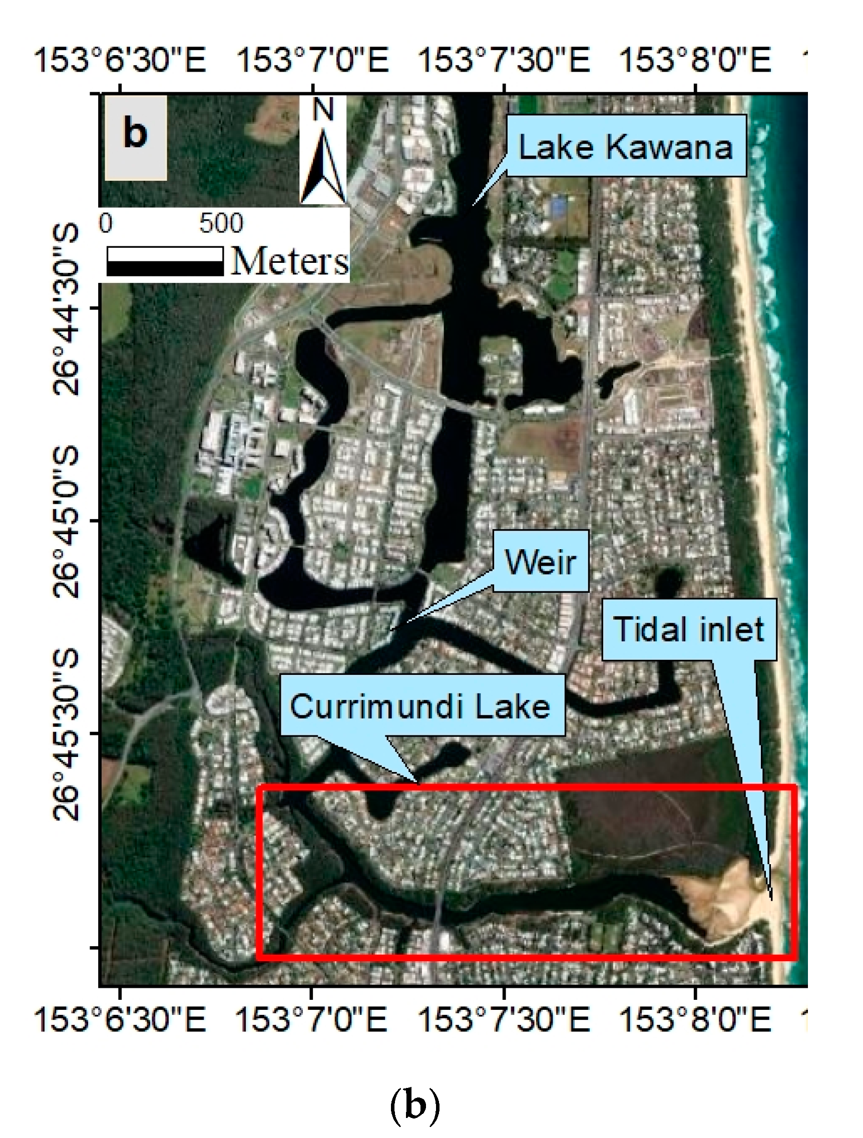
2.1. Study Area

The field study location was the main channel of Currimundi Lake. Currimundi Lake (longitude 153°8′10″ E, latitude 26°45′40″ S) is a micro-tidal estuary located in south-east Queensland characterized as a mixed tide with a predominantly semi-diurnal tidal pattern and is a micro-tidal estuary with a spring tidal range limited to 0.8 m [27]. The depth of the mid-channel varies between 3 to 5 m and the width varies from 70 to 300 m between upstream and downstream (Figure 1). Lake Kawana discharges freshwater into the Currimundi Lake system through a weir (0.65 m above the AHD) located 3.6 km from the channel mouth. When the inlet is open, the average discharge rate is 80 ML/day to maintain the water level upstream. The main channel of Currimundi Lake is connected and generally open to the ocean whilst the main tributaries and man-made water bodies are located upstream (Figure 1).

2.2. Field Experiment Descriptions and Instrumentation

The field experiment covered 2 km of a relatively straight channel reach downstream from the pontoon (Figure 1) for a 21 h period during both ebb and flood conditions (27–28 April 2015). Key environmental forcings include wind, tide, and discharge (Table 1). To obtain the flow velocity at the near-surface, both GPS-tracked floating drifters and fixed ADV were used.
Drifters utilised in this study were low-cost, low-resolution, cylindrical PVC pipes: 4 cm diameter and 50 cm long with similar physical configuration as the high-resolution drifters described in Suara, Wang [9]. The drifters were ballasted to achieve a ~47 cm submerged height. These drifters have an absolute horizontal position accuracy between 2 and 3 m and were sampled at 1 Hz. A fleet of 18 drifters was launched in Currimundi Lake on 28 April 2015 in clusters of four; they floated in the main channel for three hours from 13:00 to 16:00. Four drifters were either lost or experienced logging errors, thus data from 14 drifters were used in this study. The distance travelled by drifters between the bridge (point A) and pontoon (point B) is shown (Figure 1). The ADV was mounted 0.5 m below the water surface at the pontoon (B) and sampled continuously at 50 Hz during the entire experiment period from 19:00 on 27 April to 16:00 on 28 April (Figure 1). Further details about environmental conditions, instrumentation and quality control for this experiment are explained in [28].

2.3. Hydrodynamic Model

Hydrodynamic simulations were conducted using Delft3D FM, an open-source hydrodynamic model developed by Deltares, Netherlands. The model was run in depth-averaged 2D mode. The model solves the Navier–Stokes equations for an incompressible fluid, using the shallow water equations and the Boussinesq assumptions. To ensure that the model output is independent of the grid resolution, a grid independence test was carried out. Five different grids were constructed ranging from 25 m down to 2 m. The cross-sectional average velocity at the middle of the domain (Point C in Figure 1a) was used to test the mesh convergence. The results show that the average velocity was not sensitive to further refinement beyond a minimum grid size of 5 m. However, an increase in the minimum grid size caused an increase in the cross-sectional average velocity. Courant–Friedrichs–Lewy (CFL) condition for this model was (CFL ≤ 1). A detailed model description can be accessed through the manual [29].
Modelling at Currimundi Lake used an unstructured grid with a spatial resolution of 5 m following the channel morphology; the time series of discharge obtained from an ADV and the water level obtained from a gauging station were used for upstream and downstream boundaries, respectively. The downstream boundary was forced with water level data obtained from the tidal gauge within the main channel and sampled at an interval of five minutes. Therefore, the diurnal, semi-diurnal and higher frequency tidal constituents are included in the boundary. The simulation time step was 1 min over the simulation period of 21 h plus a 21 h spin-up time for initial condition propagation. A spatially constant bottom friction was defined by applying Manning’s coefficient n = 0.025 obtained through model calibration.
The model calibration process is a pivotal prerequisite to the DA process because DA algorithms are mainly bias-blind [30] and erroneous parameters can lead to significant uncertainties in the DA process. The calibration of the hydrodynamic model was performed with two sets of data: Eulerian calibration using 70% of velocity measurements collected from a fixed-instrument (ADV) and Lagrangian calibration using 70% velocities from GPS-tracked drifters. Both calibrations used Root Mean Square Error (RMSE) and correlation (R2) between observed and simulated velocities and aimed to adjust the bed roughness coefficient through Manning’s coefficient (n). The optimum Manning coefficient (n = 0.025) attained through Lagrangian calibration was equivalent to that observed via Eulerian calibration. Thus, Lagrangian data has the potency to be used in hydrodynamic model calibration in such environments. After the calibration, modelled and observed velocities correlated very well (R2 = 0.94) and root mean square error was reasonably low (RMSE = 0.019 m/s), suggesting that the calibration successfully reduced systematic model errors. The calibrated model was then validated by comparing simulated velocities with 30% of the measurements for both Eulerian and Lagrangian velocities. The RMSE and R2 values through this validation reflected a successful calibration of the model. The calibration and validation of the hydrodynamic model are presented in full detail in [28].
To investigate the effect of DA on the direction of residual currents in the main channel, we used our calibrated model to simulate the dynamics of Currimundi Lake for longer durations of one day, two days, four days and eight days. Upstream and downstream boundary forcings (i.e., discharge and water level) used in the hydrodynamic model for longer temporal simulations were obtained by developing a stage-discharge relationship and gauging station data measurements. Details of the tidal discharge rating curve used to predict flow discharge as well as calibration and validation of the model can be found in [31]. We performed the Lagrangian assimilation over a period of three hours for our four model scenarios with different boundary forcing temporal variations (i.e., one day, two days, four days and eight days). We then calculated the residual currents by averaging over a complete tidal cycle (12 h 25 min), considering the predominantly semi-diurnal tidal pattern in Currimundi Lake. The impact of DA on the direction of residual currents for each of the model scenarios was based on Root Mean Square Deviation (RMSD). This was then compared to identify the best DA performance when the model period increased from one to eight days whilst the assimilation period remained fixed at three hours.

3. Data Assimilation

To enable flexibility and reasonable computational cost, we utilised a variant of the Kalman filter, namely an Ensemble Kalman Filter (EnKF). The main procedure was the recursive computation of the means and covariance matrices of the ensemble system state. Since its first introduction by Evensen [32], the EnKF has been widely used in different geoscience disciplines such as oceanic [33], riverine [34], and estuarine [35] studies. The full theoretical formulation for the EnKF framework is presented in Evensen [36].

3.1. Data Assimilation Platform

OpenDA is an open-source tool, enabling the incorporation of random numerical models and observations through assimilation algorithms. It can be utilised to minimise the programming effort by enabling flexible software implementation among users (http://www.openda.org (accessed on 1 December 2020)). The OpenDA framework is validated by performing both real and synthetic DA that supports the potency of this relatively new framework launched in 2010 (OpenDA). Three main data assimilation components in OpenDA include: (i) a stochastic observer for specifying observation data used in the application and information about data uncertainty; (ii) an algorithm that itemizes the input parameters required by DA; and (iii) a stochastic model in which users identify model-related information. The complete source code is accessible via GitHub (https://github.com/OpenDA-Association/OpenDA (accessed on 1 December 2020)).
This environment supports assimilation of the available observations through the use of filtering techniques such as EnKF and particle filters. These algorithms have been successfully applied in different areas like DA of currents and salinity profiles [37], flood forecasting [38] and more recently in DA for accurate estimation of sea level anomalies (SLA) and residual currents [39,40]. These diverse applications demonstrate the efficacy of OpenDA as a generic toolbox for DA.

3.2. Data Assimilation Algorithm

At each time step, the flow model (Delft3D FM) receives real velocity data from the drifters and the shallow water model equations produce a collection of states (ensembles) representing the evolution of the processed inputs. The EnKF compares these real data to the estimated outputs to provide the best estimation of the flow state in the field.
Below, we explain the fundamentals behind the EnKF algorithm in Equations (1)–(7). The true model state based on the physical state of the lake at time t is defined as At (in our case, velocity for the entire model grid), M is the nonlinear lake system operator, ω is the noise, and U is the hydrodynamic forcing vector (here discharge and water level) for time t:
A t = M t   ( S t 1 ,   U t 1 )   +   ω t 1 .
The state-space vector, noted A ^ is an approximation by the hydrodynamic model Delft3D-FM of the true state S. The noise is added to the forcing term ω.
The forecast state is specified by S ^ f and the analysis state acquired after DA is S ^ a :
A ^ t f = H t   ( A ^ t 1 a ,   U t 1 ) .
The observation (y) equation is described as:
y t = H t   ( A t ) + ξ t .
where H is an operator connecting the state of the system to the observation and ξ is measurement noise.
The observation prediction equation is:
y ^ t = H t ( A ^ t f ) .
and the state estimation of the system obtained from DA which will be used in the next sequence as an initial condition is:
A ^ t a = A ^ t f + K t   ( y t -   y ^ t )
K is a weighting factor called Kalman gain and is considered as a balance between model and observation uncertainties [41]. K tends to decrease the error covariance of the state estimate during the analysis time:
K t = P t f H t T H t P t f H t T + R t 1 .
where R t and P f are the measurement error covariance matrix and a priori state error covariance matrix, respectively.
The EnKF is able to compute a time-varying covariance error based on the dynamics of the system. For an ensemble of forecasts (j = 1, …, N), each prone to some level of uncertainty in model processes, forcing, or initial conditions, P is:
P t f = 1 N 1 j = 1 N ( A t , j f Ā t f ) A t , j f Ā t f T .
where P t f is the forecast error covariance.

3.3. Data Assimilation Setup

The purpose of DA is essentially to characterize uncertainties [42]. The hydrodynamics of a system is modelled based on deterministic equations and the model initial conditions. However, boundary conditions are associated with uncertainties that adversely affect the performance of any calibrated model [19]. To address this issue, we included stochasticity and added noise to both velocity components as well as the water level in boundary conditions. Observations (i.e., velocity) to be assimilated were perturbed at observation locations to support the measurement errors. Ensemble forecasting produces a number of model realizations from stochastic perturbations applied to model boundary forcings and observations. These model realizations are then propagated using available observational information, which is required to reduce model uncertainty and improve its accuracy.
We introduced stochasticity to the deterministic model by using the OpenDA noise model. To fully capture the model uncertainty, an ensemble was created with a reasonably wide spread [43]; to this end, error statistics (Table 2) were designated to sufficiently spread the ensemble members.

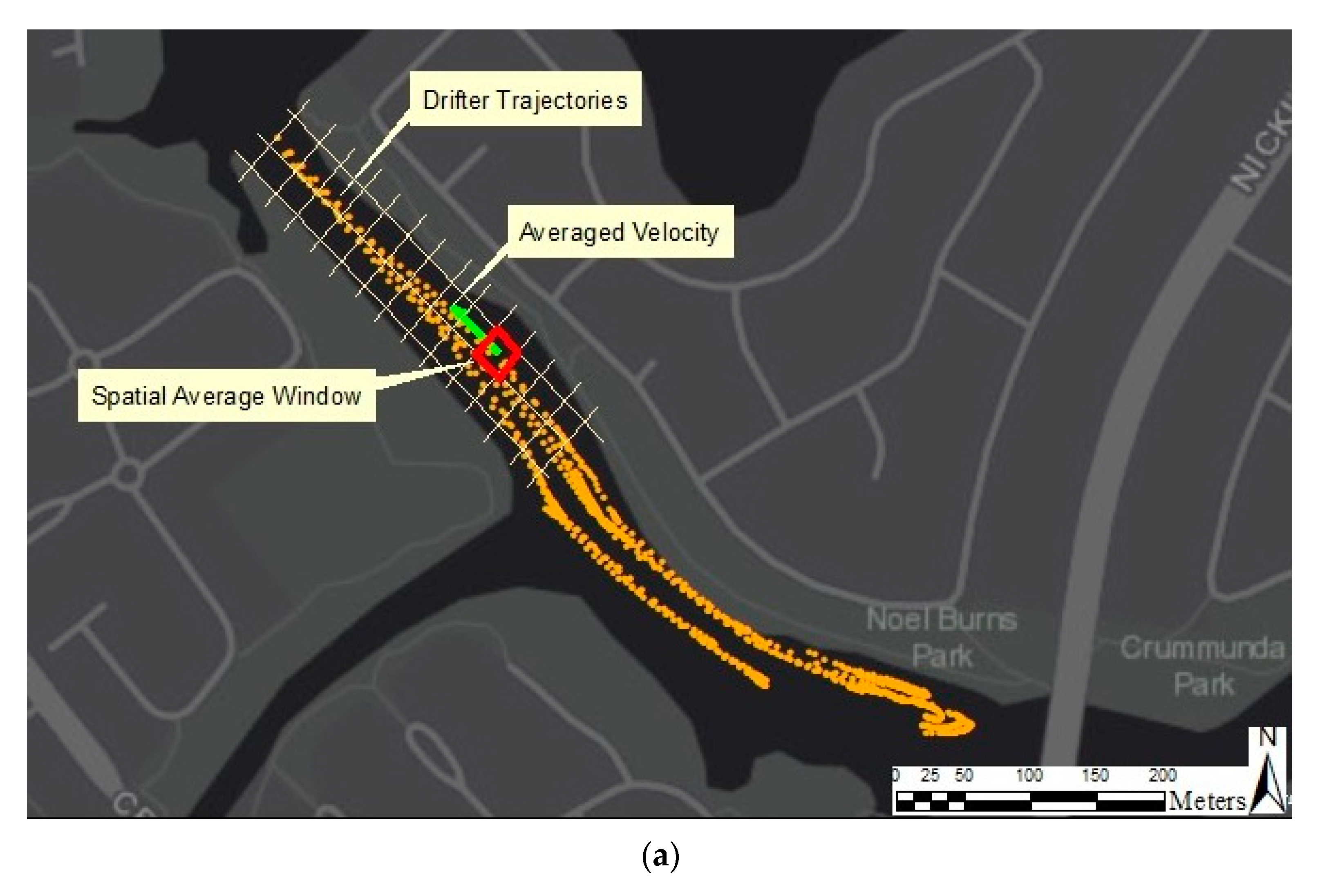
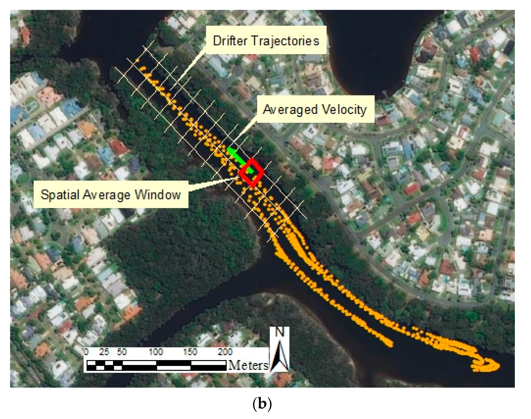
3.4. Pseudo- Lagrangian Assimilation

A common problem when assimilating Lagrangian data is that there is a nonlinear relationship between the observed variables (i.e., the positions r) and the model variables to be modified (i.e., the Eulerian velocities u). This problem can be circumvented by approximating u as the finite difference of successive positions, u ≈ Δr/Δt (Δr = position displacement and Δt = sampling period). This method, known as pseudo-Lagrangian assimilation, works well when the sampling period is much smaller than the Lagrangian correlation time scale [16]. For this study, the drifters were sampled at a frequency of 1 Hz resulting in a sampling period that is at least one order of magnitude less than the Lagrangian correlation scale (50 s) in a channel with similar physical characteristics as Currimundi Lake [9].

3.5. Trajectory Filtering

In the case of experimental flows (real data), estimated velocity (u ≈ Δr/Δt) cannot be used directly in the data assimilation system. To resolve this issue, a statistical description of individual trajectories in the form of a space–time averaging filter is applied. V a v e r a g e d   x , t is defined as the mean velocity observed at time t and location X in a space-time window W = Wt × Ws, where Wt is a temporal window around t and Ws is the spatial neighbourhood of X(t).
In Figure 2, the spatial window (red box) is indicated, representing the location of Lagrangian drifters from time t1 to time t2. As drifters move along the water, some of them enter and depart from this spatial window during the corresponding time of the window (Wt). We “average out” the velocities of all the drifters traveling through the specific spatial window during a given time interval ( V a v e r a g e d   x , t , green arrow in Figure 2. This filtered velocity represents the local flow velocity at a specified time and is subsequently used in the flow computations.
Depth averaged velocity is obtained from the drifter surface velocities using a correction factor of 0.85 following the logarithmic-law-of-the-wall for velocity profiles measurement in open channels [44].

4. DA Experiments

In this section, a base experiment (i.e., Base-Test) used as a benchmark is presented first and the rigour of the results of the Base-Test is then tested using a sensitivity analysis by varying the parameters of DA: the ensemble size, the number of the drifters and sampling period. These parameters are adjusted in an appropriate range to provide guidance for applications in real cases.
A comparison between the performance of the Lagrangian assimilation with respect to the Eulerian assimilation and Lagrangian plus Eulerian assimilation using the “pseudo-Lagrangian” scheme was conducted. Finally, the difference in the residual current direction realised by DA in terms of RMSD is presented.

4.1. Experiment Characteristics

Six different experiments were conducted to assess DA performance:
  • Free-Run: Model simulation without assimilation;
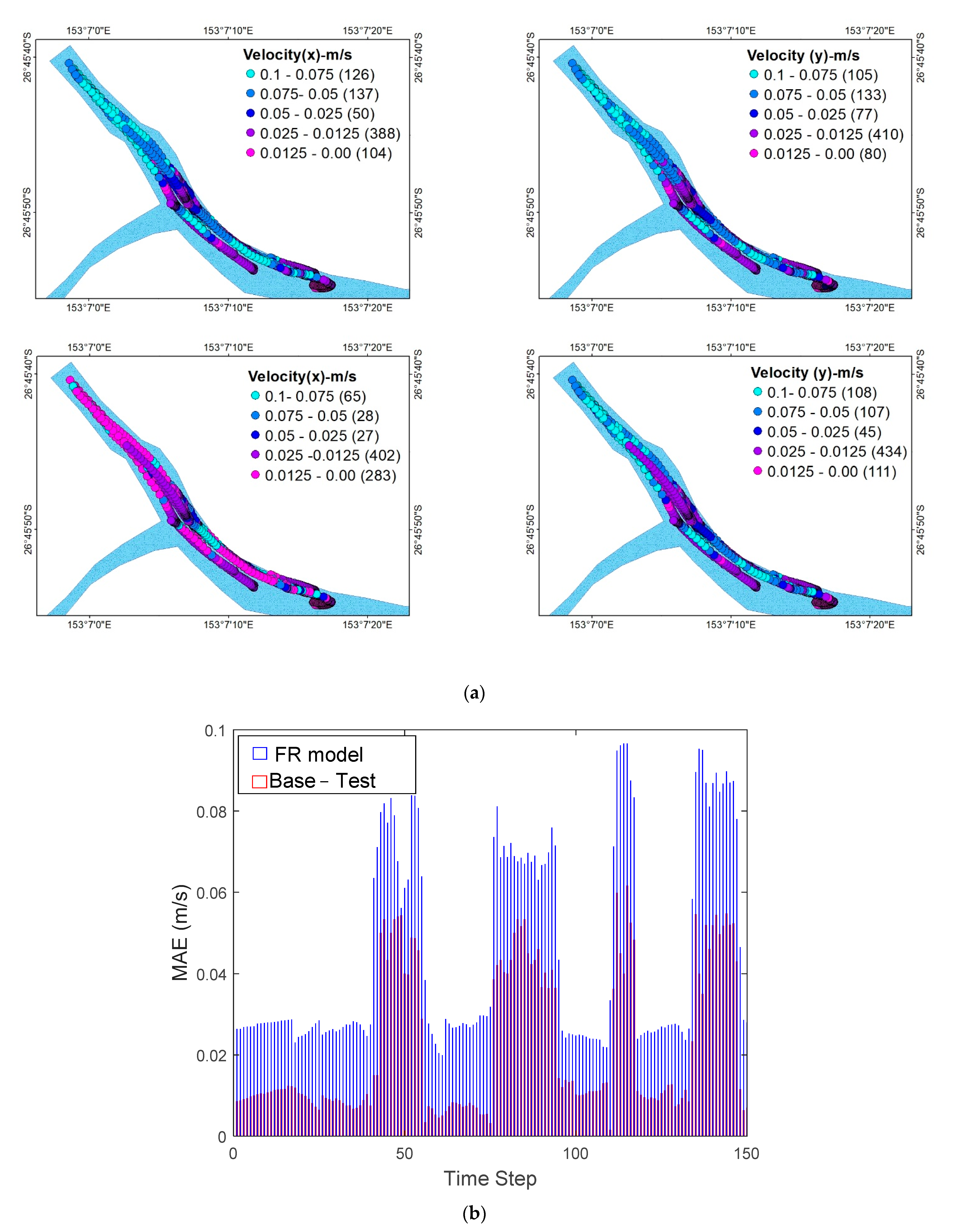
  • Base-Test: The assimilation of the Eulerian velocities obtained from eight Lagrangian drifter data released within the straight section of the channel between points A and B (Figure 1). The assimilation process initiates with a sampling period Δt = 1 min, which corresponds to the time step of the model, so the assimilation is undertaken at each model time step. This experiment is designed to study the DA performance on the velocity estimates subject to the availability of velocity information during the drifter travel time;
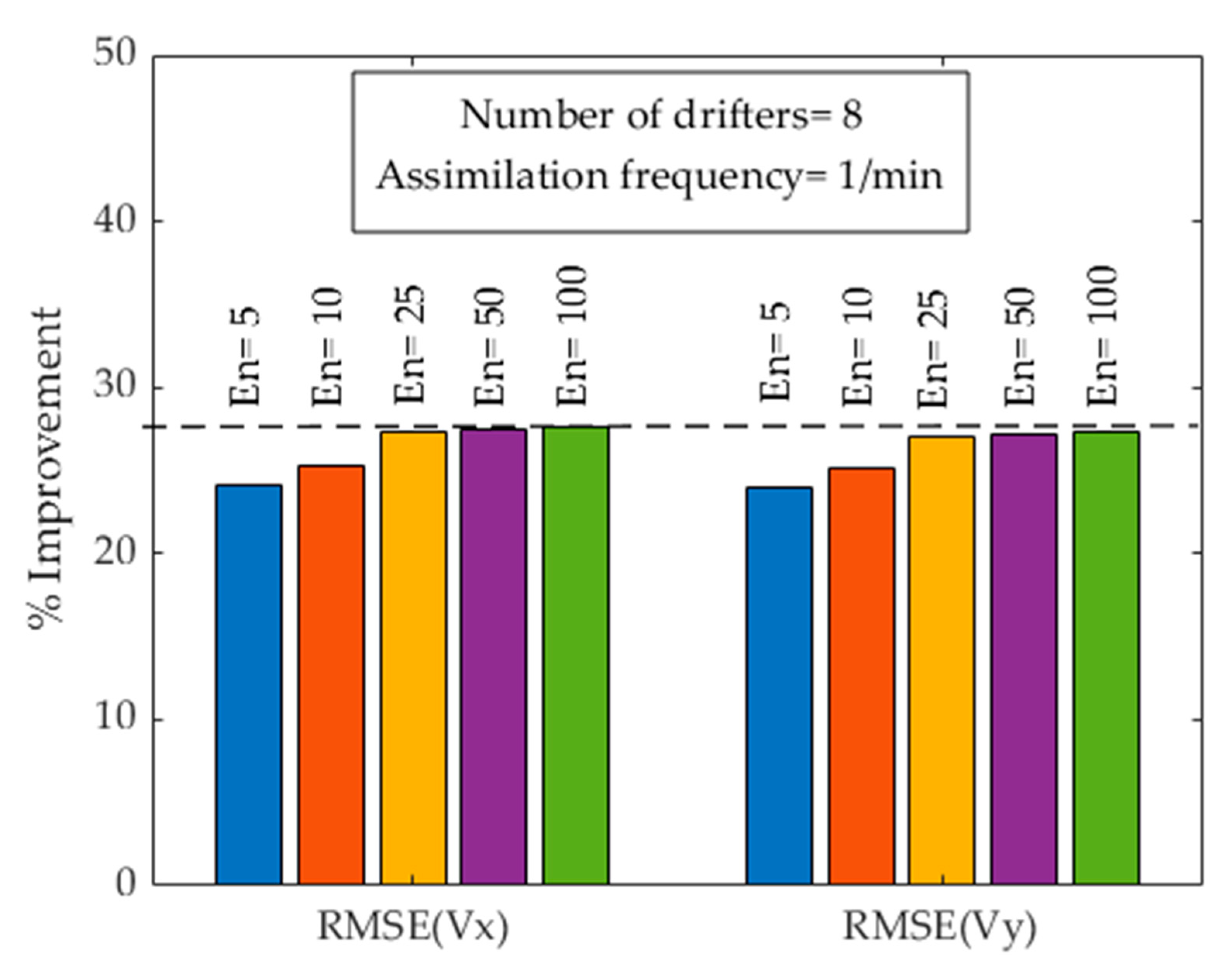
  • Ensemble-Test: To assess the impact of the number of ensemble members, five values for ensemble size were analysed: 5, 10, 25, 50 and 100. Various ensemble sizes were selected to gain the optimum size considering a trade-off between computational cost and accuracy;
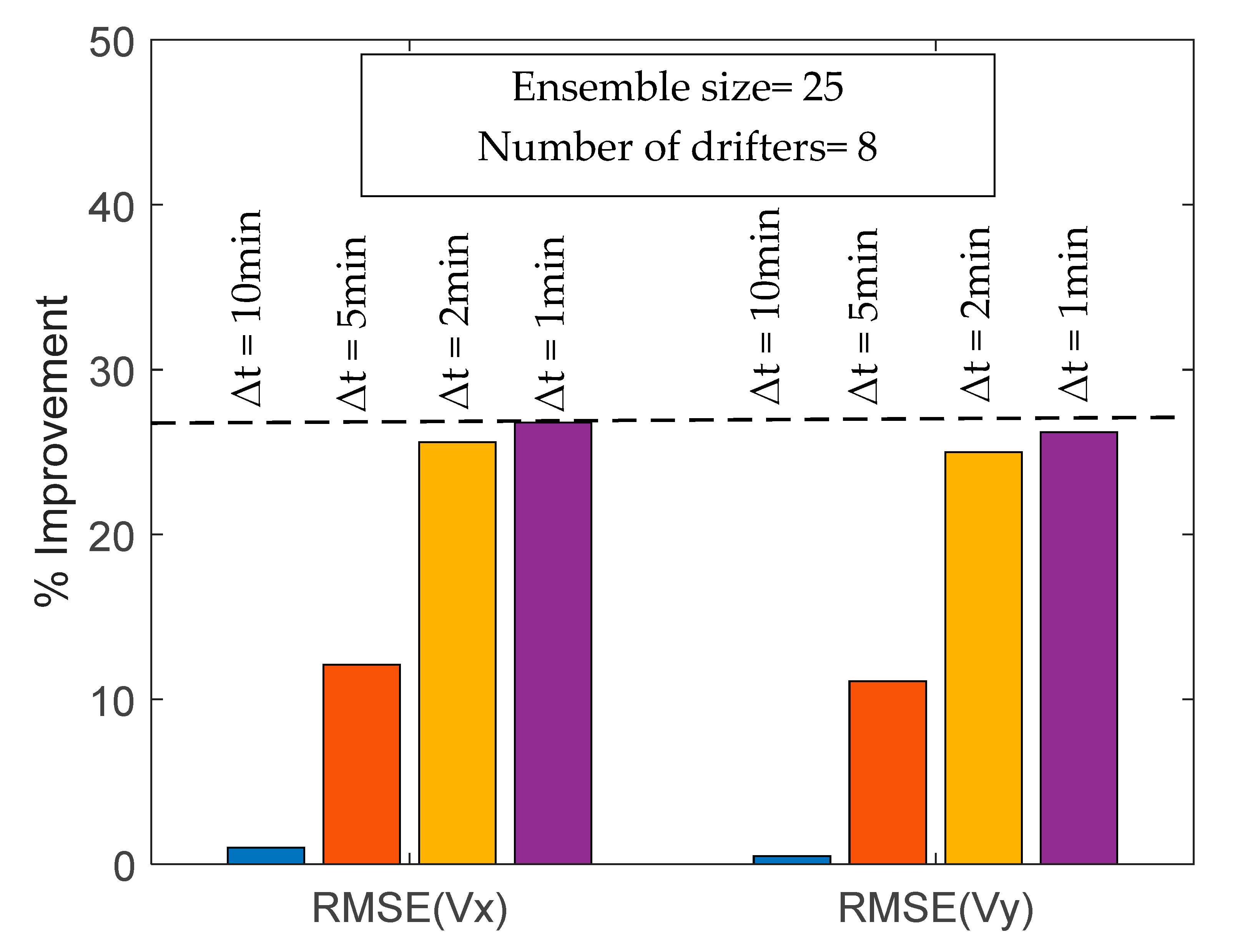
  • Frequency-Test: A series of experiments was performed maintaining the same configuration as in Base-Test, using sampling period Δt varied as 1, 2, 5 and 10 min.
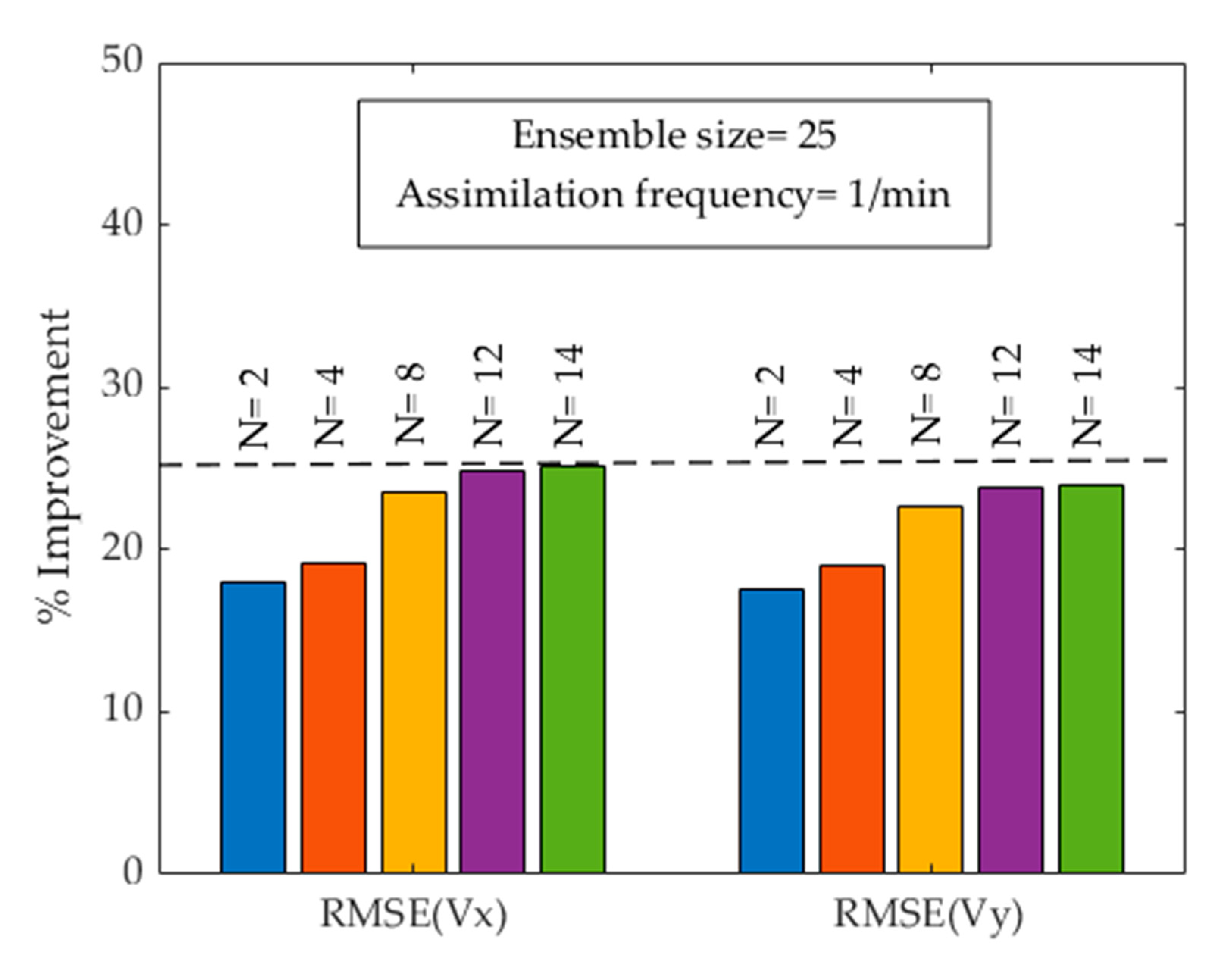
  • Density-Test: To examine the effect of the number of drifters deployed, two experiments, in addition to Base-Test, were performed with four and two drifters released in the straight section of the lake;
  • Validation-Test: To validate the DA performance with a different set of data (i.e., six non-assimilated drifters).

4.1.1. Monitoring Configurations

Depending on the availability of velocity data at various locations in the domain of interest, estimates of how the velocity improved using DA varied. By identifying two velocity monitoring configurations, we argue that increasing the density (i.e., number) and the distribution (i.e., spatial coverage) of observations in the channel will lead to improvement of velocity and residual currents results in our domain. To assess DA performance, two monitoring Set-Ups were used in addition to the Base-Test:
  • Set-Up I: Using one fixed ADV deployed 0.5 m below the surface at the pontoon (Figure 1). This set-up investigated the impact of DA on velocity estimates, assimilating 21 h of velocity data at ten-second intervals.
  • Set-Up II: A combination of Base-Test and Set-Up I, using both drifters and ADV velocity data simultaneously. Table 3 summarises the characteristics of the DA experiments and monitoring network used for evaluating the DA performance.

4.1.2. DA Performance Evaluation

The success of the assimilation in the experiments and Set-Ups is evaluated. Different measures for evaluating and comparing the results of various scenarios employed in this study are used as benchmark indicators. The velocity estimates obtained by Free-Run and Base-Test were compared with the drifter measurements in terms of RMSE at any station or location that observations were available.
Root mean square error (RMSE) is estimated as:
RMSE = 1 n   i = 1 n V s i m u l a t e d V o b s e r v e d 2  
To quantify the improvement gained by the DA, we defined percentage improvement as:
%   Improvement = [ 1 [ R M S E F r e e   R u n / R M S E E s t i m a t e ] ] × 100
Absolute Accuracy Error is calculated as:
AAE = V s i m u l a t e d V O b s e r v e d
Mean Absolute Error is calculated as:
MAE = 1 n i = 1 n V s i m u l a t e d V O b s e r v e d
Deviations between simulated velocities before and after assimilation (i.e., Free-Run and DA experiments) were used to compare the performance of DA for both Eulerian and Lagrangian assimilations (i.e., Root Mean Square Deviation (RMSD)).
The velocities in the model state are described in terms of north/east ( V x and V y ) components. The results here are presented in terms of the magnitude and direction of the currents because, operationally, these are the parameters of interest. The velocity magnitude and direction (θ) are obtained as:
V m a g = V x 2 + V y 2     ( m / s )
θ = tan 1 V y V x π × 180   ( degrees )

5. Results and Discussion

5.1. Ensemble Size

To employ a statistical sample of the state of the system, the EnKF functions by integrating ensembles of states that are independent of each other; therefore, the model is run N (number of ensembles) times. The ensemble size is generally identified empirically and is based upon a compromise between a reasonable representation of the state and computation cost [19]. Increasing the size of the ensemble (N) decreases the errors in the Monte Carlo sampling at the rate of 1 N [36]. We determined ensemble size by performing a sensitivity analysis using ensemble sizes of 5, 10, 25, 50 and 100.
With respect to our Base-Test (Section 4.1), the results indicate that for an increasing number of ensembles the analysis error reduces. Figure 3 provides RMSE for both velocity components when the size of the ensemble varies. The most striking improvement in RMSE occurs when we increase N up to 25. Further increases in the ensemble size had no significant improvement; hence, we conclude that the best improvement was achieved with 25 ensemble members.

5.2. Assimilation Frequency

An important physical parameter to consider in DA is the frequency at which data are assimilated into our model. To test the sensitivity of our DA approach to the assimilation frequency, we performed a series of experiments maintaining the same configuration as in the Base-Test with eight drifters but altering the value of the frequency (Δt) at which drifter velocities were assimilated into the model. Error estimates in terms of RMSE for both velocity components are presented in Figure 4. For assimilation intervals <2 min, our model remains less sensitive to the specific interval used, likely due to data correlation effects. However, increasing the assimilation interval beyond 2 to 10 min shows a high degradation in DA performance. This infers that DA performance is highly responsive to the frequency of data assimilation. Assimilating drifter data every 1 min resulted in ~27% improvement while assimilating every 10 min produced essentially no improvement in model output. Performing assimilations every 5 min provided an 11% and 13% improvement in V x and V y , respectively, notably less than the improvement gained in the Base-Test, with an assimilation frequency of 1 min. However, an assimilation frequency of 2 min led to a slight degradation in DA performance improvement compared to the Base-Test. In fact, increasing the time interval beyond the Lagrangian integral time scale of the lake (here, ~50 s) causes some important spatiotemporal velocity information to be lost, leading to deterioration in the model performance [16]. In general, the results denote that using a DA time interval close to the Lagrangian integral time scale of the domain leads to better outcomes.

5.3. Number of Drifters

Determining the optimal number of drifters to be deployed is an important aspect of our Lagrangian DA assessment. To this end, four experiments in addition to the Base-Test were conducted with 2, 4, 12 and 14 drifters while keeping other parameters the same as those in the Base-Test (Table 3). Error assessments in terms of RMSE for both velocity components are shown in Figure 5. A major improvement in the RMSE occurs when 14 drifters are used. However, the optimum value is attained with eight drifters because this results in the maximum improvement in RMSE with the fewest number of drifters. When the number of drifters exceeds eight, the error reduces marginally by ~2%. The optimum value of eight drifters determined here supports the selection in the Base-Test (Table 3). In all cases, DA is effective even when a limited number of drifters were used (i.e., two drifters), which affirms the value of assimilating minimal Lagrangian drifter data to improve model estimates, possibly for locations poorly covered by observation systems. This indicates that a small number of drifters can result in a significant improvement to model predictions. With more observations, our analysis shows better improvement and is, therefore, less likely to have unrealistic features in our hydrodynamic model outputs that can appear when a sparse network of observations is analysed. Although it would be more beneficial to record more data, this optimum number of drifters is dependent on many factors including the flow domain being modelled (e.g., eddy dominant or quiescent (slack) sections of the domain) [21].

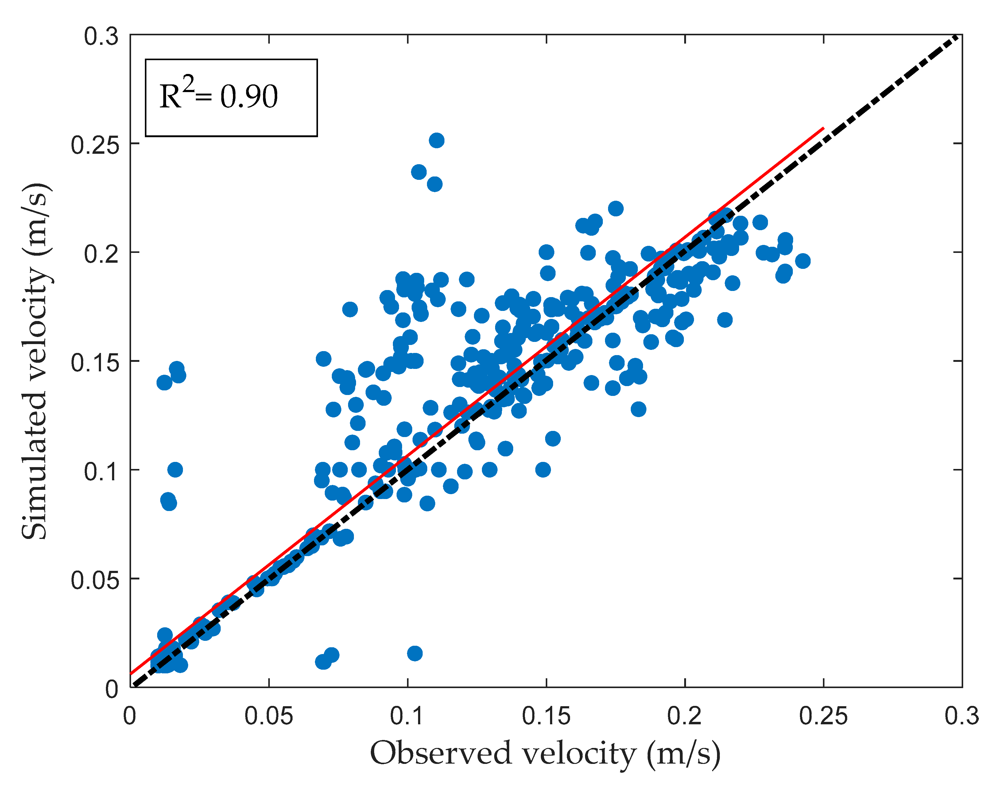
5.4. Model Validation

We validated the model using independent data, that is, data that were not assimilated by the system. We validated the DA process by comparing modelled velocity estimates when data from eight drifters were assimilated with non-assimilated observations (i.e., six drifters). It is noted that the velocity output from model simulations that was compared with measured velocities were based on the actual drifter trajectories with 1 min interval (Δt = 1). A scatter plot of observed versus simulated horizontal velocities shows good agreement (R2 = 0.90) between velocities derived from the model at drifter locations and velocities of non-assimilated drifters (Figure 6). This agreement is significantly higher than the correlation obtained between model velocity without assimilation and drifter velocities (R2 = 0.56) [28]. The result here further determines a reliable DA performance and shows that the integration of Lagrangian data significantly improves the hydrodynamic model prediction.

5.5. Improvement of Velocity Estimates at Observed Locations

DA improvement of the model estimates of velocity at all observed locations was tested. To evaluate the impact of velocity data on the efficiency of assimilation, an absolute error indicator was used. Figure 7a examines the observation minus modelled velocity components in the domain that was covered by drifters and for the x (left panels) and y components (right panels). The absolute error between observations (i.e., drifter velocities) and modelled velocities derived from the Free-Run (i.e., model without assimilation) is plotted in the top panel and the absolute error between observations and modelled velocity after assimilation (i.e., Base-Test) is shown in the bottom panel. Clearly, the DA enhanced model performance with most of the error values near zero after assimilation. The Free-Run appears to have a higher error at observed locations while the assimilation appears to have reduced this error significantly, bringing the modelled velocity close to the observed velocity. To better exhibit the general performance of the DA, Figure 7b shows the time series of absolute error for the modelled velocity with and without assimilation (i.e., Base-Test and Free-Run, respectively) with respect to drifter velocity. It is evident that assimilation of drifter velocities can successfully reduce the errors in the modelled velocity during the assimilation period.

5.6. Impact of DA Observation Types on the Model Performance

The assimilation runs were conducted for the Set-Up I and II in addition to the Base-Test which assimilated pseudo-Lagrangian drifter data. Set-Up I assimilated the Eulerian data while Set-Up II assimilated both the pseudo-Lagrangian dataset used in the Base-Test and the Eulerian dataset used in Set-Up I. DA performance with respect to the differences between model estimates with and without assimilation was examined. Velocity magnitude for the Free-Run simulation is shown in Figure 8a. The RMSD between Free-Run modelled velocities and DA modelled velocities in the Base-Test, Set-Up I and Set-Up II for all grid points was calculated. The special variation of RMSD for the Base-Test shows that DA remarkably improved the model results of Lagrangian drifter data assimilation, specifically in the sections of the lake where the drifters traversed (Figure 8b). These findings suggest that DA performance is highly dependent on the spatial coverage of drifters. Large RMSD values were observed in a small area in the vicinity of downstream boundary where no observations were available. Errors are likely due to sparse data.
The spatial variation of RMSD (i.e., the deviation between Free-Run and Set-Up I) for the assimilated velocity was then calculated. This statistical measure shows that a single sensor at a certain location can contribute to improvement in the model results through DA (Figure 8c). We found distinct differences between the model before and after assimilation. The difference between the assimilated Lagrangian and Eulerian velocity (Set-Up II) and Base-Test velocity, suggests that including both sets of data (i.e., Lagrangian and Eulerian) concurrently results in larger RMSD in the domain compared to when the Base-Test or Set-Up I is examined independently (Figure 8d). The model is strongly affected by DA as observed from the three cases examined, although the impacts are not identical in terms of magnitude or with respect to location. RMSE and R2 values before and after DA for Lagrangian, Eulerian and Both Lagrangian and Eulerian DA indicate significant improvements over the Free-Run simulation (Table 4 and Figure 9).

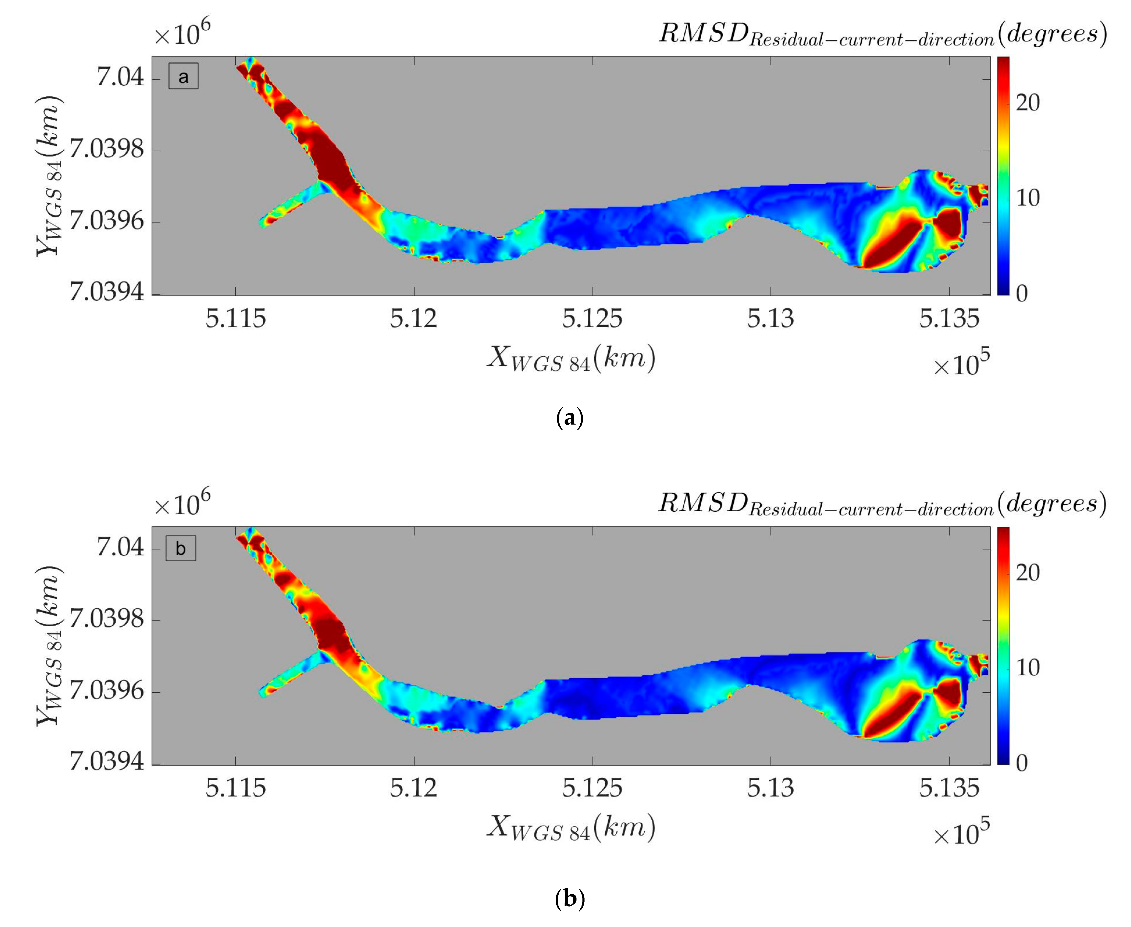
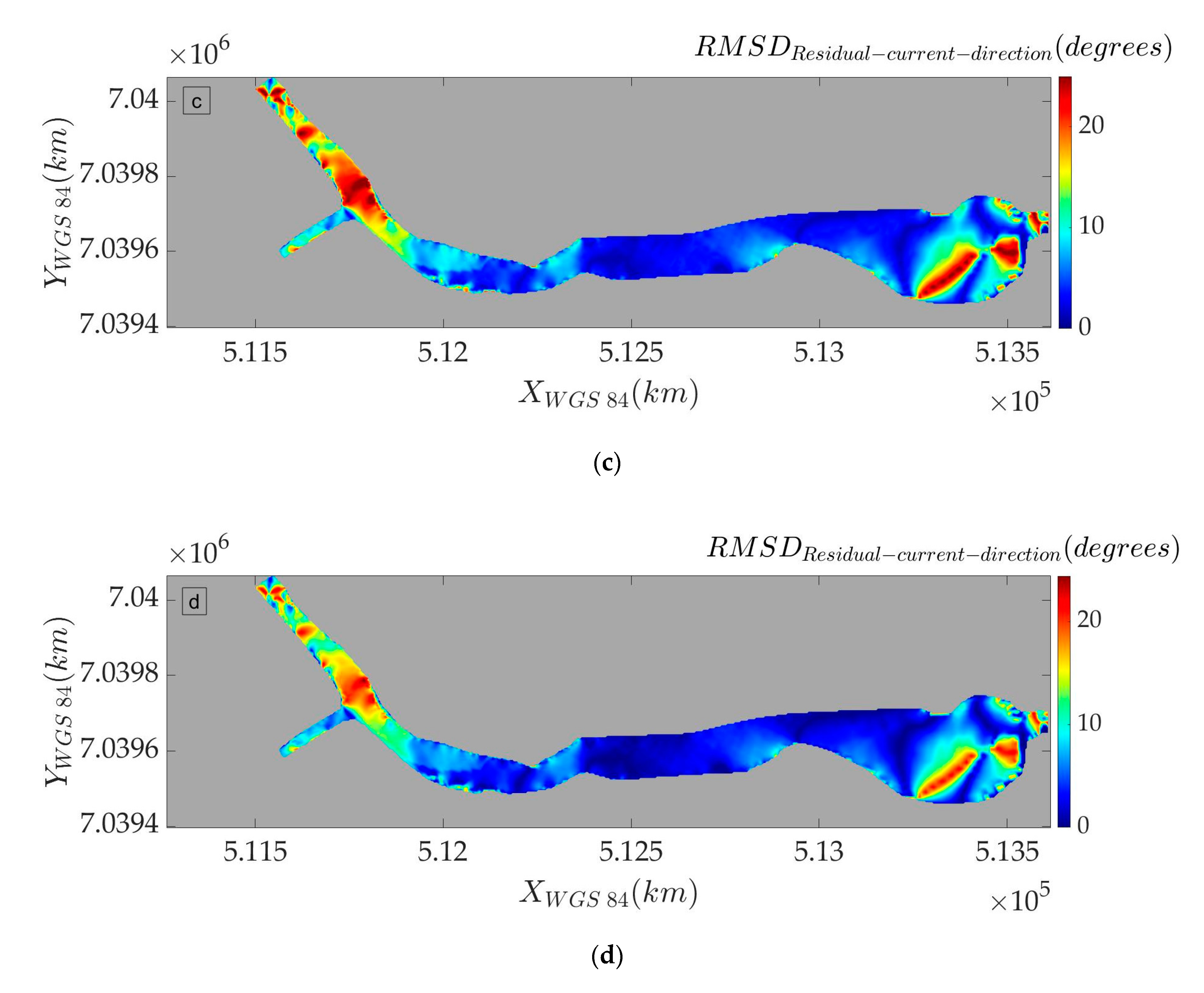
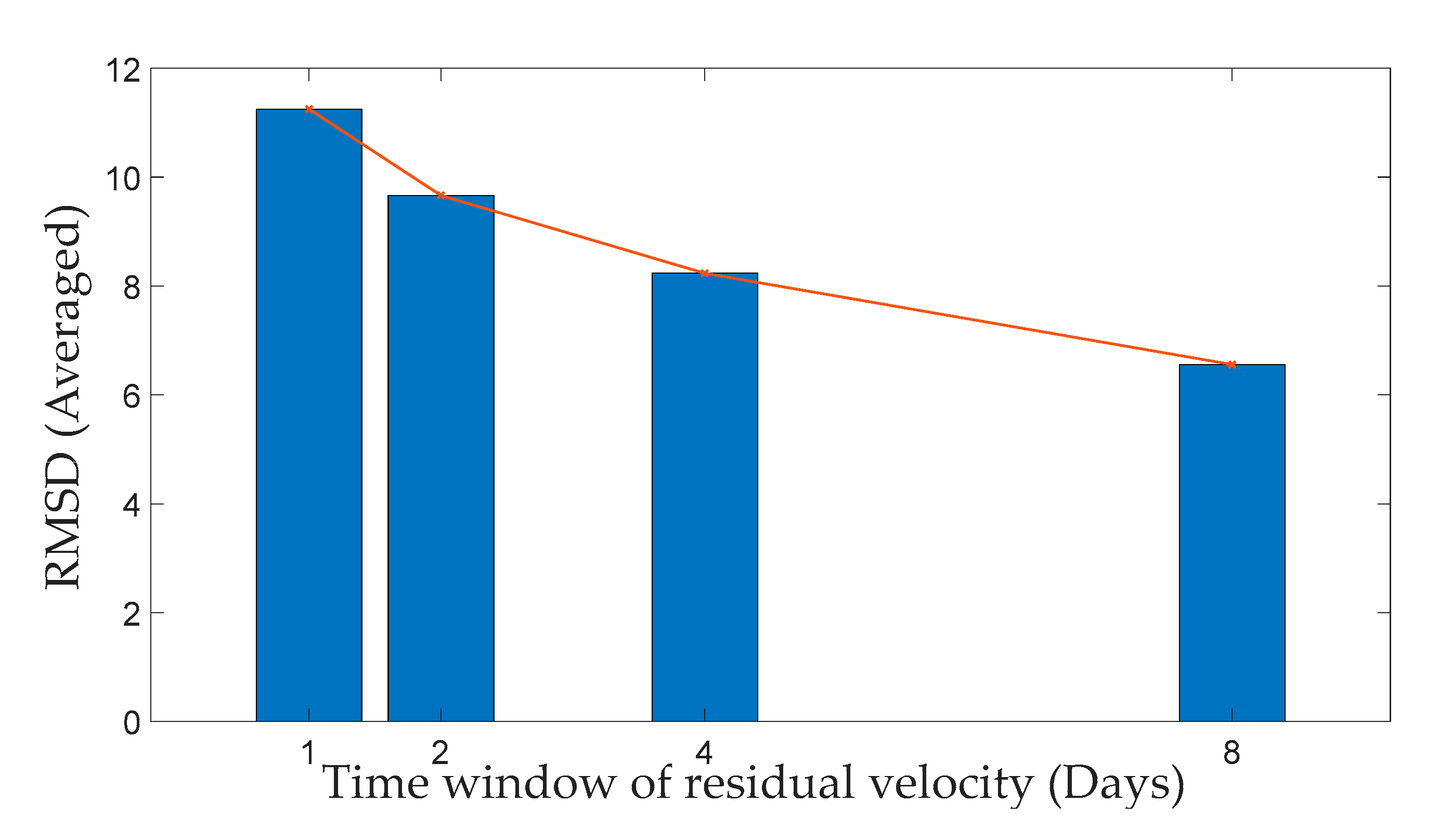
5.7. Spatial Variation of Residuals Currents (Direction of Residual Currents)

Tidal hydraulics and entrance dynamics along with bank erosion and water quality are dominant issues with high priorities that need to be addressed for Currimundi Lake. The hydrodynamic and residual transport patterns emerging from tidal motion have important consequences for the transport of sediments, water quality and bank erosion; thus, an accurate estimation of residual currents is very important in this setting.
A previously developed tidal rating curve was used to predict a long time series of discharges by measuring the water level at a gauging station. This relationship was validated by investigating the correlation between the predicted and observed discharge, along with examining the comparison between model outputs using observed and predicted discharge boundary conditions [31]. The residual currents were derived from tidal velocities during 8-day, 4-day, 2-day and 1-day periods in which full tidal cycles prevailed. These non-tidal currents driven by wind are important in estuaries because they are the principal means of transport for dissolved and suspended matter [45,46]. In addition, the lack of consistent current measurements in these areas begs the need for accurate current estimations. The effect of DA on the direction of residual currents in terms of RMSD is shown in Figure 10. While the assimilation window is kept constant at 3 h, the time window of residual velocity changes. A significant difference between the model without assimilation and Set-Up II for time windows of 1, 2, 4, and 8 days was observed (Figure 10a–d, respectively). The deviation is particularly larger in the 1-day window of residual velocity and especially in shallow sections of the lake mostly driven by wind (close to downstream boundary) and the section where drifters made their way through as expected from DA performance analysis results. Given that the assimilation period is constant, as the time window of residual velocity increases, the deviation between model results without assimilation and Set-Up II decreases, which shows the effect of the ratio of residual velocity period to assimilation period on the DA performance (Figure 11).

6. Conclusions

Drifters have a long history of use in oceanographic, climate research and weather forecasting; however, they have only been introduced into estuarine environments in the last few years. Accordingly, many drifter types exist. Recently, drifters with Global Positioning System (GPS) receivers have drawn considerable attention due to their ability to obtain data with a large spatiotemporal coverage at a relatively lower cost compared to traditional Eulerian instruments. This work provides the first examination into the use of low-cost, low-resolution Lagrangian drifters for improving the accuracy and understanding of flow field dynamics of a micro-tidal estuary (Currimundi Lake) through data assimilation into a hydrodynamic model.
The real velocities derived from the Lagrangian drifter data in addition to Eulerian velocities were assimilated into a two-dimensional version of Delft3D-FM which solves shallow water equations through a finite element method. Assimilation experiments were conducted for 3 h, using the flow data collected during the 28 April 2015 experiment. The EnKF was applied through the OpenDA assimilation toolbox. We tested the system for different data configurations and model setups. The problem of assimilation of Lagrangian drifter data in Eulerian models is circumvented by applying a pseudo-Lagrangian approach through which the corresponding Eulerian velocity is constructed. OpenDA, which is an open interface standard, was used to evaluate the efficiency of an Ensemble Kalman Filter (EnKF) data assimilation scheme to improve the velocity field and residual currents of the study domain.
The pivotal elements influencing DA performance were examined. The robustness of the EnKF method was assessed by varying several parameters, such as the number of ensembles, frequency of assimilation and number of drifters. We found that the ensemble size plays a key role in reducing model error. The results also show that DA performance is highly sensitive to the assimilation time interval, where a more frequent DA time interval of 1 min led to the largest improvement (i.e., 28%). Increasing the time interval to 10 min showed nearly no improvement because of velocity information loss. Assimilation of Lagrangian drifter data, even with a limited number of drifters, improves velocity estimates. Therefore, even a small number of Lagrangian sensors can be effective for collecting water flow information to be used in an EnKF-driven assimilation process.
The Lagrangian assimilation algorithm was examined by conducting a series of DA experiments. A base experiment (Base-Test) was performed using data from eight drifters in the model. The results obtained by Lagrangian assimilation were compared with Eulerian and Lagrangian plus Eulerian assimilation. Results demonstrated the efficacy of DA performance because a significant deviation was gained in velocity maps before and after assimilation. We found that both Lagrangian and Eulerian data improve assimilation of our system dynamics with Lagrangian data being the most important. The results also indicate that concurrent assimilation of Lagrangian drifter and Eulerian ADV velocities lead to a higher deviation between assimilated and non-assimilated models.
Our results suggest that a desirable alternative to fixed Eulerian devices such as ADVs and ADCPs are drifters. Furthermore, drifters can be promptly deployed in any specific domain under study, particularly in the case that unforeseen events occur. Lagrangian measurements are especially beneficial in the areas where Eulerian instruments are either sparse or unreliable. It is evident, however, that directly assimilating Lagrangian positions is relatively difficult in Eulerian-based hydrodynamic models because of the differences in data and model frameworks. In addition, raw Lagrangian data are rather challenging to use because particle flow is generally affected by local flow perturbations, which are induced by different physical processes, such as turbulence and surface wind. Despite these inherent challenges, the work showed that the use of low-cost, low-resolution drifters provided relatively higher improvement in the model prediction over the Eulerian data set due to a larger area coverage.
Using a discharge-rating curve, we predicted discharge for the period of 1, 2, 4, and 8 days, which was then applied to model the domain for these time periods. The direction of residual currents was calculated over the full tidal cycles, which showed better results (i.e., the deviation between model before and after assimilation) when the time window of assimilation decreased from 8 days to 1 day and demonstrated large differences in the shallow areas as well as the section captured by drifters. Having an open connection with the ocean, these non-tidal currents are not necessarily initiated internally but are often propagated from the ocean. Depending on the availability of estuary stage data, this study can be conducted during major tidal periods and therefore can act as a guidance platform for assessing the role of DA in improving the modelled currents for the entire spatial extension of the domain.

Author Contributions

All authors (N.M., M.K., K.S., R.B., A.M. and R.C.S.) designed and performed the experiment. N.M. and K.S. analysed the data. N.M. wrote the manuscript. All authors interpreted the data, discussed and edited the manuscript. All authors have read and agreed to the published version of the manuscript.

Funding

This research was funded by the Australian Research Council through Linkage grant LP150101172.

Acknowledgments

The authors acknowledge the financial supports received from the Australian Research Council through Linkage grant LP150101172 as well as the Sunshine Coast Council for providing access to station data. The authors gratefully acknowledge the contribution of Paul Boswood from Qld Department of Environment and Science in reviewing the manuscript. The authors would also like to thank USC and QUT staff and volunteer undergraduates who participated in the field study.

Conflicts of Interest

The authors declare no conflict of interest.

References

  1. Babovic, V.; Karri, R.; Wang, X.; Ooi, S.K.; Badwe, A. Efficient data assimilation for accurate forecasting of sea-level anomalies and residual currents using the Singapore regional model. Paper presented at the Geophys. Res. Abstr. 2011, 13. [Google Scholar]
  2. Baracchini, T. From Observations to 3D Forecasts: Data Assimilation for High Resolution Lakes Monitoring; EPFL: Lausanne, Switzerland, 2019. [Google Scholar]
  3. Baracchini, T.; Chu, P.Y.; Šukys, J.; Lieberherr, G.; Wunderle, S.; Wüest, A.; Bouffard, D. Data assimilation of in situ and satellite remote sensing data to 3D hydrodynamic lake models: A case study using Delft3D-FLOW v4.03 and OpenDA v2.4. Geosci. Model Dev. 2020, 13, 1267–1284. [Google Scholar] [CrossRef] [Green Version]
  4. Barnard, P.L.; Erikson, L.H.; Elias, E.P.; Dartnell, P. Sediment transport patterns in the San Francisco Bay Coastal System from cross-validation of bedform asymmetry and modeled residual flux. Mar. Geol. 2013, 345, 72–95. [Google Scholar] [CrossRef]
  5. Bellsky, T.; Kostelich, E.J.; Mahalov, A. Kalman filter data assimilation: Targeting observations and parameter estimation. Chaos Interdiscip. J. Nonlinear Sci. 2014, 24, 024406. [Google Scholar] [CrossRef] [PubMed] [Green Version]
  6. Chanson, H.; Brown, R.J.; Trevethan, M. Turbulence measurements in a small subtropical estuary under king tide conditions. Environ. Fluid Mech. 2012, 12, 265–289. [Google Scholar] [CrossRef] [Green Version]
  7. Cormier, R.; Kannen, A.; Elliott, M.; Hall, P.; Davies, I.M. Marine and Coastal Ecosystem-Based Risk Management Handbook; International Council for the Exploration of the Sea (ICES): Copenhagen, Denmark, 2013. [Google Scholar]
  8. D-Flow Flexible Mesh User Manual. Manuals Delft3D FM Suite 2019.01. Available online: https://www.deltares.nl/en/software/delft3d-flexible-mesh-suite/ (accessed on 1 December 2020).
  9. Dee, D.P. Bias and data assimilation. Q. J. R. Meteorol. Soc. 2005, 131, 3323–3343. [Google Scholar] [CrossRef] [Green Version]
  10. El Serafy, G.Y.; Gerritsen, H.; Hummel, S.; Weerts, A.H.; Mynett, A.E.; Tanaka, M. Application of data assimilation in portable operational forecasting systems—the DATools assimilation environment. Ocean Dyn. 2007, 57, 485–499. [Google Scholar] [CrossRef] [Green Version]
  11. Elliott, M.; Borja, A.; McQuatters-Gollop, A.; Mazik, K.; Birchenough, S.; Andersen, J.H.; Painting, S.; Peck, M. Force majeure: Will climate change affect our ability to attain Good Environmental Status for marine biodiversity? Mar. Pollut. 2015, 95, 7–27. [Google Scholar] [CrossRef] [Green Version]
  12. Evensen, G. Sequential data assimilation with a nonlinear quasi-geostrophic model using Monte Carlo methods to forecast error statistics. J. Geophys. Res. Space Phys. 1994, 99, 10143–10162. [Google Scholar] [CrossRef]
  13. Evensen, G. The Ensemble Kalman Filter: Theoretical formulation and practical implementation. Ocean Dyn. 2003, 53, 343–367. [Google Scholar] [CrossRef]
  14. Fraccascia, S.; Winter, C.; Ernstsen, V.B.; Hebbeln, D. Residual currents and bedform migration in a natural tidal inlet (Knudedyb, Danish Wadden Sea). Geomorphology 2016, 271, 74–83. [Google Scholar] [CrossRef]
  15. Garcia, M.; Ramirez, I.; Verlaan, M.; Castillo, J. Application of a three-dimensional hydrodynamic model for San Quintin Bay, B.C., Mexico. Validation and calibration using OpenDA. J. Comput. Appl. Math. 2015, 273, 428–437. [Google Scholar] [CrossRef]
  16. Garel, E.; Ferreira, O. Fortnightly Changes in Water Transport Direction Across the Mouth of a Narrow Estuary. Chesap. Sci. 2012, 36, 286–299. [Google Scholar] [CrossRef]
  17. Gauss, F. Theory of the Motion of Heavenly Bodies Moving about the Sun in Conic Sections; (English transl. by CH Davis), reprinted 1963; Dover: New York, NY, USA, 1809. [Google Scholar]
  18. Honnorat, M.; Monnier, J.; Le Dimet, F.-X. Lagrangian data assimilation for river hydraulics simulations. Comput. Vis. Sci. 2008, 12, 235–246. [Google Scholar] [CrossRef] [Green Version]
  19. Koch, M.; Sun, H. Tidal and non-tidal characteristics of water levels and flow in the Apalachicola Bay, Florida. WIT Trans. Built Environ. 1970, 43, 10. [Google Scholar]
  20. Le Coz, J.; Hauet, A.; Pierrefeu, G.; Dramais, G.; Camenen, B. Performance of image-based velocimetry (LSPIV) applied to flash-flood discharge measurements in Mediterranean rivers. J. Hydrol. 2010, 394, 42–52. [Google Scholar] [CrossRef] [Green Version]
  21. Loos, S.; Shin, C.M.; Sumihar, J.; Kim, K.; Cho, J.; Weerts, A.H. Ensemble data assimilation methods for improving river water quality forecasting accuracy. Water Res. 2019, 171, 115343. [Google Scholar] [CrossRef]
  22. MacMahan, J.; Brown, J.; Thornton, E. Low-Cost Handheld Global Positioning System for Measuring Surf-Zone Currents. J. Coast. Res. 2009, 253, 744–754. [Google Scholar] [CrossRef]
  23. Mardani, N.; Suara, K.; Fairweather, H.; Brown, R.; McCallum, A.; Sidle, R.C. Improving the Accuracy of Hydrodynamic Model Predictions Using Lagrangian Calibration. Water 2020, 12, 575. [Google Scholar] [CrossRef] [Green Version]
  24. Mardani, N.; Suara, K.; Khanarmuei, M.; Brown, R.; McCallum, A.; Sidle, R. A Numerical Investigation of Dynamics of A Shallow Intermittently Closed and Open Lake and Lagoon (ICOLL). In Proceedings of the 22nd Australasian Fluid Mechanics Conference AFMC2020, Brisbane, Australia, 7–10 December 2020. [Google Scholar]
  25. Mcsweeney, S.; Kennedy, D.M.; Rutherfurd, I.D. Classification of Intermittently Closed and Open Coastal Lakes and Lagoons in Victoria, Australia. In Proceedings of the 7th Australian Stream Management Conference, Townsville, Australia, 27–30 July 2014. [Google Scholar]
  26. Molcard, A.; Piterbarg, L.I.; Griffa, A.; Özgökmen, T.M.; Mariano, A.J. Assimilation of drifter observations for the reconstruction of the Eulerian circulation field. J. Geophys. Res. Space Phys. 2003, 108, 3058. [Google Scholar] [CrossRef] [Green Version]
  27. Molcard, A.; Poje, A.C.; Özgökmen, T.M. Directed drifter launch strategies for Lagrangian data assimilation using hyperbolic trajectories. Ocean Model. 2006, 12, 268–289. [Google Scholar] [CrossRef]
  28. Németh, A.A.; Hulscher, S.J.; de Vriend, H.J. Modelling sand wave migration in shallow shelf seas. Cont. Shelf Res. 2002, 22, 2795–2806. [Google Scholar] [CrossRef]
  29. Oubanas, H.; Gejadze, I.; Malaterre, P.-O.; Mercier, F. River discharge estimation from synthetic SWOT-type observations using variational data assimilation and the full Saint-Venant hydraulic model. J. Hydrol. 2018, 559, 638–647. [Google Scholar] [CrossRef]
  30. Pawlowicz, R.; Hannah, C.; Rosenberger, A. Lagrangian observations of estuarine residence times, dispersion, and trapping in the Salish Sea. Estuarine Coast. Shelf Sci. 2019, 225, 106246. [Google Scholar] [CrossRef]
  31. Sakov, P.; Sandery, P.A. Comparison of EnOI and EnKF regional ocean reanalysis systems. Ocean Model. 2015, 89, 45–60. [Google Scholar] [CrossRef]
  32. Salman, H.; Kuznetsov, L.; Jones, C.K.R.T.; Ide, K. A Method for Assimilating Lagrangian Data into a Shallow-Water-Equation Ocean Model. Mon. Weather. Rev. 2006, 134, 1081–1101. [Google Scholar] [CrossRef] [Green Version]
  33. Shaha, D.C.; Cho, Y.-K.; Kwak, M.-T.; Kundu, S.R.; Jung, K.T. Spatial variation of the longitudinal dispersion coefficient in an estuary. Hydrol. Earth Syst. Sci. 2011, 15, 3679–3688. [Google Scholar] [CrossRef] [Green Version]
  34. Song, Z.; Shi, W.; Zhang, J.; Hu, H.; Zhang, F.; Xu, X. Transport Mechanism of Suspended Sediments and Migration Trends of Sediments in the Central Hangzhou Bay. Water 2020, 12, 2189. [Google Scholar] [CrossRef]
  35. Suara Wang, C.; Feng, Y.; Brown, R.J.; Chanson, H.; Borgas, M. High-resolution GNSS-tracked drifter for studying surface dispersion in shallow water. J. Atmos. Ocean. Technol. 2015, 32, 579–590. [Google Scholar] [CrossRef] [Green Version]
  36. Suara Wang, H.; Chanson, H.; Gibbes, B.; Brown, R.J. Response of GPS-tracked drifters to wind and water currents in a tidal estuary. IEEE J. Ocean. Eng. 2018, 44, 1077–1089. [Google Scholar] [CrossRef] [Green Version]
  37. Suara, K.; Mardani, N.; Fairweather, H.; McCallum, A.; Allan, C.; Sidle, R.; Brown, R. Observation of the Dynamics and Horizontal Dispersion in a Shallow Intermittently Closed and Open Lake and Lagoon (ICOLL). Water 2018, 10, 776. [Google Scholar] [CrossRef] [Green Version]
  38. Tamura, H.; Bacopoulos, P.; Wang, D.; Hagen, S.C.; Kubatko, E.J. State estimation of tidal hydrodynamics using ensemble Kalman filter. Adv. Water Resour. 2014, 63, 45–56. [Google Scholar] [CrossRef]
  39. Tinka, A.; Strub, I.; Wu, Q.; Bayen, A.M. Quadratic programming based data assimilation with passive drifting sensors for shallow water flows. Int. J. Control. 2010, 83, 1686–1700. [Google Scholar] [CrossRef]
  40. Tossavainen, O.-P.; Percelay, J.; Tinka, A.; Wu, Q.; Bayen, A.M. Ensemble Kalman Filter based state estimation in 2D shallow water equations using Lagrangian sensing and state augmentation. In Proceedings of the 47th IEEE Conference on Decision and Control, Cancun, Mexico, 9–11 December 2008; pp. 1783–1790. [Google Scholar] [CrossRef]
  41. Van Velzen, N.; Verlaan, M. COSTA a problem solving environment for data assimilation applied for hydrodynamical modelling. Meteorol. Z. 2007, 16, 777–794. [Google Scholar] [CrossRef]
  42. Voulgaris, G.; Meyers, S.T. Temporal variability of hydrodynamics, sediment concentration and sediment settling velocity in a tidal creek. Cont. Shelf Res. 2004, 24, 1659–1683. [Google Scholar] [CrossRef]
  43. Wang, X.; Karri, R.; Ooi, S.; Babovic, V.; Gerritsen, H. Improving predictions of water levels and currents for Singapore regional waters through data assimilation using OpenDA. In Proceedings of the 34th World Congress of the International Association for Hydro-Environment Research and Engineering: 33rd Hydrology and Water Resources Symposium and 10th Conference on Hydraulics in Water Engineering, Brisbane, Australia, 26 June–1 July 2011. [Google Scholar]
  44. Weerts, A.H.; El Serafy, G.Y.; Hummel, S.; Dhondia, J.; Gerritsen, H. Application of generic data assimilation tools (DATools) for flood forecasting purposes. Comput. Geosci. 2010, 36, 453–463. [Google Scholar] [CrossRef]
  45. Wu, Q.; Tinka, A.; Weekly, K.; Beard, J.; Bayen, A.M. Variational Lagrangian data assimilation in open channel networks. Water Resour. Res. 2015, 51, 1916–1938. [Google Scholar] [CrossRef]
  46. Zhang, D.; Madsen, H.; Ridler, M.E.; Kidmose, J.; Jensen, K.H.; Refsgaard, J.C. Multivariate hydrological data assimilation of soil moisture and groundwater head. Hydrol. Earth Syst. Sci. 2016, 20, 4341–4357. [Google Scholar] [CrossRef] [Green Version]
Figure 1. (a) Aerial view of Currimundi Lake main channel including instruments and observation locations. Drifters were deployed at point A and removed at point B. (b) Aerial view of Currimundi Lake catchment including Lake Kawana and the weir separating Currimundi Lake and Lake Kawana (Maps created using ArcGIS software (Esri, 2020)).
Applsci 11 11006 g001aApplsci 11 11006 g001b
Figure 2. Outline of spatial–temporal averaging to remove small velocity fluctuations from Lagrangian drifters. The red box is the space-time window W, the drifter trajectories are denoted by orange dots, and the green arrow indicates the averaged velocity.
Applsci 11 11006 g002aApplsci 11 11006 g002b
Figure 3. Sensitivity of DA performance to ensemble size. Five different ensembles were examined according to the Base-Test configuration.
Applsci 11 11006 g003
Figure 4. Sensitivity of DA performance to frequency of assimilation. Drifter data were assimilated at 1, 2, 5 and 10 min intervals. The Base-Test configuration is applied.
Applsci 11 11006 g004
Figure 5. Sensitivity of DA performance to number of drifters complied with the Base-Test configuration.
Applsci 11 11006 g005
Figure 6. Comparison between modelled velocities and the velocities of non-assimilated drifter data.
Applsci 11 11006 g006
Figure 7. (a) Absolute error between modelled and observed velocities before assimilation (top) and after assimilation (bottom) for the V x (left) and V y components (right) of velocity. Numbers in brackets indicate the frequency of data in each category. (b) Time series of absolute error between modelled velocities and observations before and after assimilation.
Applsci 11 11006 g007
Figure 8. DA effect on velocity magnitude in the entire domain. (a) Model without assimilation, (b) the difference between model estimates with and without assimilation according to Base-Test configuration, (c) using configuration Set-Up I and (d) Set-Up II.
Applsci 11 11006 g008aApplsci 11 11006 g008b
Figure 9. Scatter plots of modelled versus observed velocity (m/s) for Lagrangian (Base-Test), Eulerian (Set-Up I) and Lagrangian and Eulerian (Set-Up II) assimilation.
Applsci 11 11006 g009
Figure 10. Residual velocity calculated for: (a) 1-day, (b) 2-day, (c) 4-day and (d) 8-day periods; the assimilation window is 3 h in all cases.
Applsci 11 11006 g010aApplsci 11 11006 g010b
Figure 11. The effect of residual velocity time window on averaged root mean square error.
Applsci 11 11006 g011
Table 1. Overview of environmental conditions and instrumentation.
Inlet ConditionDateTideTidal Range (m)Water Elevation
(m)
Discharge Range (m3/s)Wind Speed Range (m/s)Instrument DeployedSample Frequency
(Hz)
Open27 April 2015Ebb0.40.20.6–170–4.0ADV- Sontek-2D side-looking (16 MHz)50
Open28 April 2015Flood/Ebb0.60.70.15–300–4.0LR, low cost drifter 1
Table 2. Noise model parameters.
ParameterDescriptionValue
σ W l   (m)Water level standard deviation0.05
σ D i s c h a r g e   ( m 3 / s ) Discharge standard deviation1
ρ W l   (h)Water level temporal correlation6
ρ D i s c h a r g e   (h)Discharge temporal correlation6
Table 3. Characteristics and Parameters of the Experiments.
ExperimentAssimilation TypeMeasurement Type and NumberMeasurement LocationAssimilation Duration and Frequency
Free-Runxxxx
Base-TestPseudo Lagrangian8 driftersFrom point A to B in Figure 13 h */1 min
Ensemble testPseudo Lagrangian8 driftersFrom point A to B in Figure 13 h/1 min
Frequency testPseudo Lagrangian8 driftersFrom point A to B in Figure 13 h/1 min
Density testPseudo Lagrangian8 driftersFrom point A to B in Figure 13 h/1 min
Validation testPseudo Lagrangian6 driftersFrom point A to B in Figure 13 h/1 min
Set-Up IEulerian1 ADVPoint C near bridge in Figure 118 h/1 min
Set-Up IIEulerian + Pseudo Lagrangian8 drifters + 1 ADVFrom point A to B and Point C in Figure 121 h/1 min
* Time that drifters travelled in channel.
Table 4. Summary of the data assimilation performance (RMSE).
Free-Run
No Assimilation
Base-Test
DA with Lagrangian Data
Set-Up I
DA with Eulerian Data
Set-Up II
DA with Lagrangian & Eulerian Data
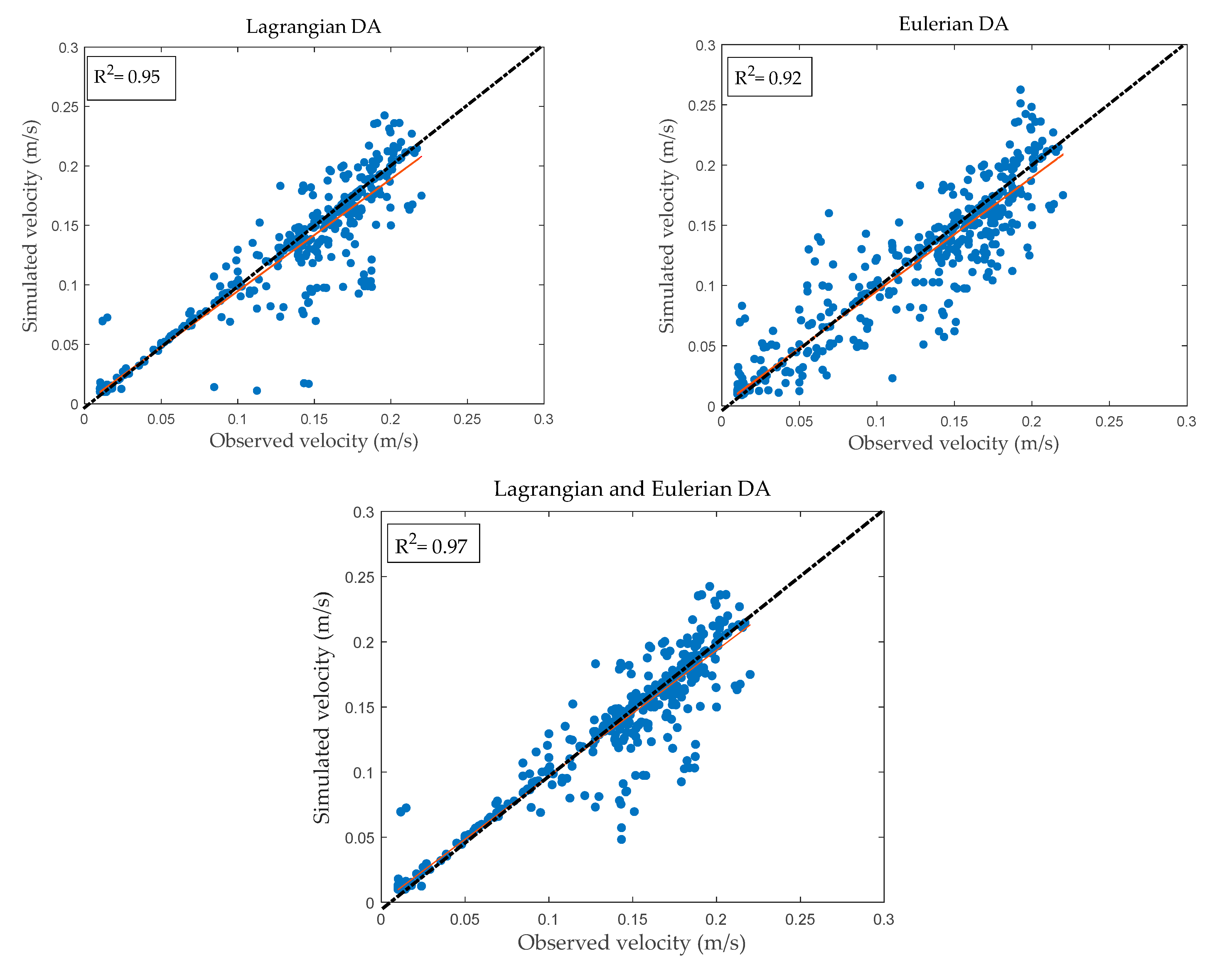
RMSE (m/s)0.070.050.0590.043
R20.560.950.920.97
Improvement (%) 281639
Publisher’s Note: MDPI stays neutral with regard to jurisdictional claims in published maps and institutional affiliations.

