Numerical Modelling of Flow-Debris Interaction during Extreme Hydrodynamic Events with DualSPHysics-CHRONO

Abstract

Floods can transport debris of a very wide range of dimensions, from cohesive sediments to large floating debris, such as trees and cars. The latter increases the risk associated with floods by, for example, obstructing the flow or damaging structures due to impact. The transport of this type of debris and their interaction with structures are often studied experimentally in the context of tsunamis and flash floods. Numerical studies on this problem are rare, therefore the present study focuses on the numerical modelling of the flow-debris interaction. This is achieved by simulating multiple laboratory experiments, available in the literature, of a single buoyant container transported by a dam-break flow in order to validate the chosen numerical approach. The numerical simulations are carried using the open source DualSPHysics model based on the smoothed particle hydrodynamics method coupled with the multi-physics engine CHRONO, which handles the container–bottom interactions. The trajectory, as well as the velocity of the centroid of the container, were tracked throughout the simulation and compared with the same quantities measured in the laboratory. The agreement between the model and the experiment results is quantitatively assessed using the normalised root mean squared error and it is shown that the model is accurate in reproducing the floating container trajectory and velocity.

1. Introduction

Tsunami events such as the one occurred in Japan in 2011 in Tohoku [1] and the ones in Indonesia in 2004 and 2018 [2] resulted in catastrophic consequences on coastal communities and structures causing many casualties. Studies in the literature often focused on the impact of tsunamis on the coastal region [3,4,5,6,7]. However, recent research investigated the effects that debris transported by such tsunamis can have on existing structures, especially after the damage documented during the 2011 Tohoku tsunami. Using the evidence found after this event a debris hazard classification was developed by Naito et al. [8] by analysing the damages caused by different debris types. Among the types with most energetic estimated impact forces on structures were shipping containers, especially loaded ones. Forces between 1500 and 6400 kN were estimated by Naito et al. [8] on structures by applying the FEMA P646 [9] guidelines for the design of structures. These recommend a formula for the calculation of the maximum force exerted by floating debris based on the Haehnel and Daly [10] relationship. In the wake of the 2011 Tohoku tsunami, further relationships were incorporated in the American Society for Civil Engineers (ASCE) [11] design codes and provide a simplified model for large floating debris impact forces for structural design, accounting also for impact orientation based on the mean impact orientation of Haehnel and Daly [10]. However, important factors such as debris material are not yet taken into account in any design guideline to date.

In order to have more detailed models for large floating debris dynamics, a large number of studies focused on investigating their behaviour when entrained in a flow, e.g., trajectories, spreading, orientation etc. [1,12,13,14,15] or on analysing their impact forces during a collision with a structure [16,17,18,19]. More recently Derschum et al. [20] and Stolle et al. [21,22] studied both processes in conjunction by using a single “smart debris” [23] shaped as a 1:40 geometrically scaled 20 ft standard container to analyse both the trajectories and the impact forces on a structure with the aim of improving the reliability of design guidelines for structures that may be exposed to such hazards and to serve as benchmark tests for future numerical simulations.

The numerical modelling of these processes is rare in the literature [24] with significant limitations in the numerical methods used. Initial studies on solid-fluid interactions for debris were conducted by Wu et al. [25]. They used Navier–Stokes equations coupled with Volume Of Fluid (VOF) to track the free surface, an approach very often used in modelling fluid-structure impacts (see, e.g., De Finis et al. [26]), and a large eddy simulation turbulence model. The motion of the floating body was modelled with a Discrete Element Method (DEM) model validating it with laboratory experiments. However, implementations of floating body mechanisms on mesh-based models are usually very challenging, requiring ad hoc formulations for specific cases and long processing times [27]. Due to these difficulties, Lagrangian particle-based methods, such as the Moving Particle Semi-implicit method (MPS) [28] or the Smoothed Particle Hydrodynamics method (SPH) [29] are often used as good alternatives to mesh-based methods [30,31]. SPH, due to its formulation, is well suited to investigate high energy phenomena since it is capable of modelling violent flows as well as flow particle detachments in the context of tsunamis [32,33]. However, even if these methods produced accurate results for solid–fluid interactions [31,34] they do not inherently account for solid body contact laws, i.e., this contact requires a specific sub- or coupled model. Canelas et al. [35] and successively [36] expanded an SPH solver via coupling with a DEM model which was validated with PVC cubes subject to a flow, but showed limitations in correctly simulating the friction between moving and boundary elements of the simulations. This was further shown in Goseberg et al. [37] which modelled experiments from Nistor et al. [15]. The combined use of SPH and DEM clearly resulted in negligible variations of debris dynamics when changing the kinematic friction coefficient f_c of the materials. Additionally, DEM implementation was also prone to numerical instabilities, also resulting in high computation times.

In order to address the aforementioned issues, the newly implemented DualSPHysics-CHRONO coupling in DualSPHysics v5.0 [38,39] is used to model the container trajectories measured in Stolle et al. [21,22]. This is, additionally, a first necessary step to study the feasibility of such approach and successively extending their use for flow-debris-structure interactions. DualSPHysics is chosen due to its advantage over other SPH numerical models of using the computational power of the Graphics Processing Unit (GPU) of a PC to speed up simulation times up to 146 times [38]. CHRONO [40,41] is a multi-physics engine that allows to solve rigid or deformable contacts and impacts between solids. In addition, it includes the possibility of integrating different types of constraints as recently done by Tagliaferro et al. [42] to simulate a planing hull. In contrast to the DEM implementation, CHRONO allows for a realistic frictional behaviour due to the inclusion of a full Coulomb sliding/sticking/rolling model. Additionally, the application of different types of constraints such as joints, hinges and springs allows to include complex structures allowing to realistically model the ones found in coastal regions or in harbours. Another advantage is the increased numerical stability gained when compared with DEM coupling.

The main objective of this work is to validate the coupling of DualSPHysics and CHRONO with the experiments presented in Stolle et al. [22]. First, the modelling of the hydrodynamics of the flow is validated, then a sensitivity analysis of the modelling of the details of the debris geometry and description of the material characteristics on the debris dynamics is carried out. Finally, the results of the calibrated models are presented and discussed.

The remainder of the manuscript is organized as follows. The explanation of the methodology, illustrating the numerical setup along with a brief introduction on the numerical methodology used is presented in Section 2. In Section 3 the main results of the initial hydrodynamics validation and subsequent calibration and validation of the debris dynamics are presented. Finally, in Section 4, the results are analysed, and the feasibility of this numerical approach is discussed in relation to potential applications for debris-structure interactions and conclusions of the work are given.

2. Methodology

For the present study, DualSPHysics v5.0 [29,38,39] coupled with CHRONO Engine are used to solve the hydrodynamics and simultaneously consider the collisions and interactions between container and floor.

2.1. DualSPHysics

DualSPHysics [39] is based on Weakly Compressible SPH (WCSPH) with the fluid phase governed by the Navier–Stokes equations, reduced to ordinary differential equations solved in a Lagrangian framework. The conservation of mass and momentum is expressed as [29,43]:

$$\frac{\mathrm{d}\rho }{\mathrm{d}t}=-\rho \nabla ·\mathit{v}$$

(1)

$$\frac{\mathrm{d}\mathit{v}}{\mathrm{d}t}=-\frac{1}{\rho }\nabla p+\mathit{g}+\mathit{\Gamma }$$

(2)

where $\rho$ is the fluid density, $t$ is time, $p$ is the pressure, $\mathit{v}=\left(v_x,v_y,v_z\right)$ is the velocity vector, $\mathit{g}=\left(g_x,g_y,g_z\right)$ is the gravitational acceleration vector (here $g_x=0,g_y=0, g_z=-9.81$ m/s² is used) and $\mathit{\Gamma }$ groups all the dissipative terms that can be defined by using two different formulations, i.e., artificial viscosity [44] or laminar with sub-particle scale turbulence formulations [45].

SPH discretises every part of the computational domain into sets of particles carrying different properties such as density, pressure, velocity, etc. In general, two steps are defined to apply Equations (1) and (2) to the SPH method, i.e., a kernel approximation and a particle approximation [46]. First, any variable $f$ of a particle $a$, located at ${\mathit{r}}_a=\left(x_a,y_a,z_a\right)$, is represented by an integral at location $\mathit{r}=\left(x,y,z\right)$

$$f\left({\mathit{r}}_a\right)={\int }_{\Omega }f\left(\mathit{r}\right)W\left({\mathit{r}}_a-\mathit{r},h_p\right)\mathrm{d}\mathit{r}$$

(3)

with $\Omega$ as the computation domain, $W$ as a weighting function called smoothing kernel, which monotonically decreases with distance, and $h_p$ as the smoothing length which determines the size of the kernel support.

In the second step, the integral in Equation (3) is approximated by interpolating the characteristics of the surrounding particles as:

$$f\left({\mathit{r}}_a\right)\approx {\displaystyle \sum }_{b}f\left({\mathit{r}}_b\right)\frac{m_b}{{\rho }_b}{W}_{ab}$$

(4)

where the summation is extended to all the particles inside the kernel. In Equation (4), $W_{ab}$=$W\left({\mathit{r}}_a-{\mathit{r}}_b,h_p\right)$, and $m_b$ and ${\rho }_b$ are the mass and density of a neighbour particle $b$ (located at ${\mathit{r}}_b=(x_b,y_b,z_b$)). In addition, any derivative of $f$ can be expressed as

$$\nabla f\left({\mathit{r}}_a\right)\approx {\displaystyle \sum }_{b}f\left({\mathit{r}}_b\right)\frac{m_b}{{\rho }_b}{\nabla }_a{W}_{ab}$$

(5)

where ${\nabla }_a$ indicates derivation with respect to the coordinates of particle $a$. Equation (1) is rewritten in the SPH framework for a particle $a$ as

$$\frac{\mathrm{d}{\rho }_a}{\mathrm{d}t}={\rho }_a {\displaystyle \sum }_b\frac{m_b}{{\rho }_b}{\mathit{v}}_{ab}·{\nabla }_a{W}_{ab}$$

(6)

A more extensive analysis of the SPH governing equations and model can be found in the reference literature [38,39,46,47,48].

2.2. CHRONO Engine and Coupling with DualSPHyics

The multi-physics engine CHRONO [40,41], coupled with DualSPHysics, is here used to solve the interaction between the container and the bottom of the flume. In the problem at hand, i.e., the transport of a container by dam-break flow, the container first becomes floating during the initial mobilisation by the flow then it impacts with the bottom and, subsequently, slides along the flume floor.

CHRONO is able to consider multiple types of structural constraints. CHRONO solves collisions through two alternative formulations, (i) Non-SMooth Contacts (NSMC), which considers fully rigid impacts, and (ii) SMooth Contacts (SMC) which solves deformable contacts. For NSMC only the restitution coefficient $K$ and the kinetic friction coefficient $f_c$ are used as variables when solving interactions between solids. SMC additionally considers Young’s modulus $E$ and the Poisson’s ratio $\nu$. In the present study (ii) is used to approximate as closely as possible the real behaviour for all materials and elements involved.

The coupling between the two models is defined with a message passing interface such that DualSPHysics first calculates the interaction between fluid particles and, subsequently, computes the fluid–floating interactions for a defined $t$. CHRONO is activated when mechanical constraints between floating bodies and/or material properties are defined as input of the simulation. In this case, both the linear and angular accelerations, together with the length of the time step $\Delta t$ in SPH are passed to CHRONO. This model computes and applies forces and momentum of the flow to the floating bodies by integrating the fluid contributions with the defined dynamics or kinematic restriction, including possible collisions. If the time step used for CHRONO is the same as for DualSPHysics, then the computation reverts to the latter with CHRONO communicating linear and angular velocities, as well as the position of the centre of mass of every floating body. In DualSPHysics the floating bodies particles positions, velocity and density are then updated considering CHRONO output. The entire system is then updated starting the cycle over again for $t+\Delta t$.

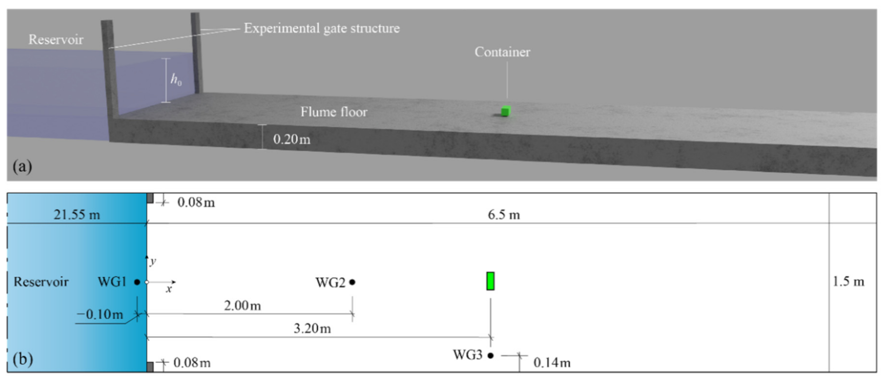
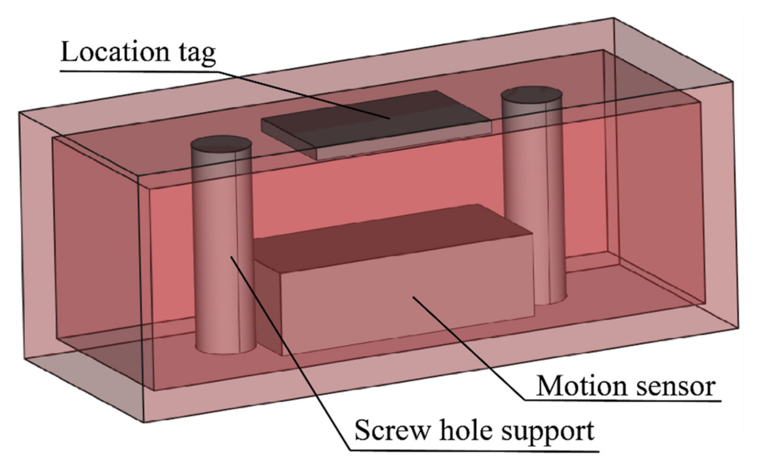
2.3. Modelled Experiments

The experimental setup described in Stolle et al. [22] is modelled herein due to its focus on container dynamics. The experiments were conducted in a 30 × 1.5 m flume. A reservoir 21.55 m long was filled with an impoundment depth of $h_0=0.4$ m and the water was released via a swing gate to generate a dam-break flow on an 8.45 m long test area with the horizontal concrete floor elevated by 0.2 m from the flume bottom. Note that, only the first 6.50 m of the experimental test area were modelled because the impact with the structure at the end of the area described in Stolle et al. [21] is not the focus of the present study. The area modelled herein is shown in Figure 1. The swing gate structure consisted of two 0.05 × 0.05 m metal columns with an additional 0.03 m ledge towards the inside of the flume covered in rubber to ensure a watertight seal. This resulted in a 0.08 m protrusion on each side of the gate slightly obstructing the dam-break flow and generating three dimensional effects [49]. The container x-coordinate of the geometrical centre was positioned on the false floor, respectively, at $x=3.2$ m from the end of the reservoir (see Figure 1). Two main orientations of the container are investigated with the longer dimension transversal (OR1) or longitudinal (OR2) in respect to the direction of propagation of the flow. The container was positioned by hand before every experimental run and centred to the flume width resulting in a mean position of the geometric centre of $y=-$0.0225 m and $y=-$0.0327 m ($y=0$ being the main axis of the flume) of $x$ = +3.2010 m and $x$ = +3.2003 m ($x=0$ being the initial position of the initial waterfront) for OR1 and OR2, respectively. Wave gauges were placed at WG1 ($x=-0.1$ m), WG2 ($x=2.0$ m) and WG3 ($x=3.2$ m) [20,21].

2.4. Numerical Setup

The numerical setup closely reproduced the experimental conditions, with two exceptions: i.e., the swing gate was approximated by using an instantaneous release of the water in the reservoir at $t$ = 0 s and the gate structure was modelled as two 0.08 × 0.05 m rectangular columns as shown in Figure 1. Note that the coordinate axis in the transversal direction of the flume is mirrored with respect to the one used by Stolle et al. [22]. First, the hydrodynamics was calibrated to define the best combination of parameters to accurately simulate the experimental hydrodynamic conditions. All the most relevant parameters defined after initial calibration are summarised in

Table 1. DualPSHysics parameters and formulations used.

Parameter	Value
dp (m)	0.01
Total number of particles	28.9 × 106
Smoothing kernel	Wendland, 1995 [50]
$h_l/dp$	1.73
Dissipative term	Artificial viscosity [44]
${\alpha }_{ff}$	0.04
$vis{c}_{bf}$	9
Density diffusion term	Fourtakas et al. 2020 [51] (only between fluid particles)

, for the remaining fundamental parameters default values were used.

A final particle spacing ($dp$) of 0.01 m was chosen as 0.02 m resulted in a higher tip of the flow (due to the larger size of the particles). A convergence test showed that results for $dp<$ 0.01 m converged to those for $dp=$ 0.01 m at the expense of a significant increase in computational time by increasing from 28 × 10⁶ particles with $dp=$ 0.01 m to 54 × 10⁶ particles with $dp=$ 0.008 m. $dp=$0.01 m was also used as the dimensions of every element of the numerical setup is a multiple of $dp$, allowing correct element sizes. Here the relationship, $h_l=\mathrm{Coefh} \sqrt{3d{p}^2}$, was used to calculate the smoothing length $h_l$ with $\mathrm{Coefh}$ being a calibration coefficient. Here $\mathrm{Coefh}=1$ was used since was already validated for dam-break flows. Note that, this value resulted in a ratio between the smoothing length and the particle spacing $h_l/dp=1.73$ (Table 1) which was also chosen by Tan et al. [32] to simulate landslide tsunamis and considered suitable for the problem at hand. In this work no sensitivity analysis on the effect of this ratio on the modelling was carried out.

In this study, to account for dissipation, i.e., to compute the $\Gamma$ term in Equation (2), the artificial viscosity formulation [44] is applied since it was also successfully used to model other extreme hydrodynamic phenomena such as landslide-tsunami [52,53]. The artificial viscosity parameter between fluid particles ${\alpha }_{ff}$ was defined as $0.04$ after initial calibration to ensure a coherent velocity of the dam break in relation to the experimental values. An additional calibration was performed for the viscosity between fluid and boundary particles ${\alpha }_{fb}=vis{c}_{bf}\times {\alpha }_{ff}$, with $vis{c}_{bf}$ being a viscosity multiplication factor. In this study $vis{c}_{bf}$ = 9 was used to approximate the roughness of the flume floor, which was covered in a paint/sand mixture, resulting in an estimated Darcy-Weisbach friction factor n = 0.014 [49]. $vis{c}_{bf}$ was calibrated making sure that velocity with the distance and arrival time of the flow to each wave gauge was reproduced accurately. Additionally, a density diffusion term was added to the continuity equation, i.e., Equation (6) by using the formulation of Fourtakas et al. [51] on the fluid particles. This additional term is commonly used to deal with density oscillations that are distinctive of SPH often resulting in incorrect and unstable pressure on boundaries or floating bodies.

The container was simulated with dimensions of 0.15 × 0.06 × 0.06 m and a mass of 0.226 kg [22]. For the initial position in y-direction, the mean values of all experiments for each orientation were used. Since the mass distribution was not symmetrical in the experiments, the container was 3D modelled as shown in Figure 2. The container trajectories and velocities shown in the paper are referred to the centroid of the container. The inertia of the container was first calculated in DualSPHysics by modelling the container as in Figure 2 with a $dp$ = 0.0005 m. This had the only purpose of letting DualSPHysics compute very accurately the inertia matrix (i.e., the 3 × 3 matrix of the moments of inertia). Since it was known that the mass distribution in the container was not symmetrical and the position of the centre of mass was not known from the experiments, this position was prescribed and calibrated with the experimental data. An eccentricity between 0.0025 m and 0.004 m in the longer dimension was considered in a series of calibration tests, with the latter value giving the best results and therefore used in the present study. The addition of the eccentricity resulted in a larger effect at the onset of the container motion with differences noticeable mainly in the y-direction; the differences in terms of centroid velocity along the y-direction (which have maxima of order of 10⁻¹ m/s) are up to 0.134 m/s at the motion onset and they become negligible after the container stabilised in the dam break flow. The centre of mass and inertia, taken from the high-resolution inertia matrix computation were subsequently prescribed at the start of each full-size simulation where a solid container was used due to particle size restrictions.

Finally, every simulation was performed on a Windows server equipped with a Nvidia Tesla P40 24 GB GPU, Intel Xeon Silver 4108 and 64 GB of Random Access Memory (RAM). With this configuration, 5 s of simulated time resulted in approximately 13 h of computing time applying the coupled DualSPHysics-CHRONO model.

2.5. Properties of the Materials

Attention was given to the material properties (see Section 2.2) used in the simulations and summarised in

Table 2. Material properties values used with CHRONO with SMooth Contacts.

Property	Container (HMWPE)	Flume Floor (Concrete + Sand Paint)
$E$ (Gpa)	0.8	30
$\nu$ (-)	0.4	0.2
$K$ (-)	0.6–0.75	0.6–0.75
$f_c$ (-)	0.125–0.2	0.3–0.5

, to ensure a realistic response to the debris-bottom interactions. High Molecular Weight Polyethylene (HMWPE) was used in the experiments [21] for which the design values of $E$ and $\nu$ [54,55] are used in the simulations (Table 2). The floor of the test area was made of concrete. However, since no information on the type of concrete was available, both $E$ and $\nu$ were chosen to reproduce the characteristics of a low strength concrete, which is considered realistic due to its non-structural role in the experimental setup.

The remaining two parameters $K$ and $f_c$ were varied in the ranges specified in Table 2. The reason behind this choice was twofold. First, these two parameters might vary with specific conditions of the experimental setup (e.g., lubricated friction) and second to understand their effects on the container dynamics.

2.6. Model Performance Assessment

The accuracy of the numerical simulation results of the flow depth ($h$) of the $x$ and $y$ trajectories of the container was assessed by using the root mean square error normalised with $h_0$ (${\mathrm{nRMSE}}_{\mathrm{l}}$) as

$${\mathrm{nRMSE}}_{\mathrm{l}}=\frac{\sqrt{\frac{1}{N}{{\displaystyle \sum }}_i^N{\left({\xi }_{n,i}-{\xi }_{e,i}\right)}^2}}{h_0}$$

(7)

where ${\xi }_{n,i}$ and ${\xi }_{e,i}$ represent any i-th sample of one of the numerically modelled and experimental variables, respectively, and N is the number of samples. Furthermore, the accuracy of the simulated $x$ and $y$ velocity components of the container ($v_x$ and $v_y$, respectively) was assessed with a root mean square error normalised with the shallow water velocity (${\mathrm{nRMSE}}_{\mathrm{v}}$) as

$${\mathrm{nRMSE}}_{\mathrm{v}}=\frac{\sqrt{\frac{1}{N}{{\displaystyle \sum }}_i^N{\left(v_{n,i}-v_{e,i}\right)}^2}}{\sqrt{g{h}_0}}$$

(8)

where $v_{n,i}$ and $v_{e,i}$ represent the numerical and experimental velocity components, respectively, in either $x$- or $y$-directions.

Two further metrics for assessing modelling performance are used in Section 4, namely the modulus of the mean error ($\left|\mathrm{ME}\right|$) defined as

$$\left|\mathrm{ME}\right|=\left|{\displaystyle \sum }_i^N\left({\xi }_{n,i}-{\xi }_{e,i}\right)/N\right|$$

(9)

and the mean distance error ($\mathrm{MDE}$) as

$$\mathrm{MDE}=\frac{1}{N} {{\displaystyle \sum }}_i^N\sqrt{{\left(x_{n,i}-x_{e,i}\right)}^2+{\left(y_{n,i}-y_{e,i}\right)}^2}$$

(10)

where the subscript n and e, representing a numerical and experimental quantity, respectively, are used to further quantify the simulations performance by comparing them with the accuracy of the positioning system used in Stolle et al. [22]. The two parameters $\left|\mathrm{ME}\right|$ and $\mathrm{MDE}$ (following Equation (16) in Stolle et al. [56]) are chosen because they are the same ones used by Stolle et al. [56] to test the accuracy of the optical tracking algorithm used for the experimental measurements presented hereinafter.

3. Results

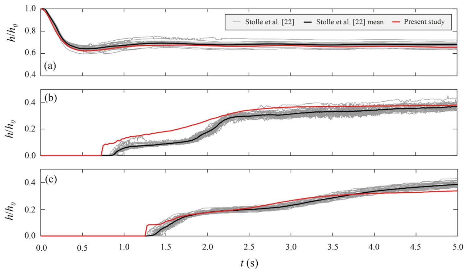
3.1. Dam Break Hydrodynamics

The hydrodynamics modelling is validated by comparing the numerical time series of the flow depth with the mean experimental one (Section 2.3) measured by Stolle et al. [22]. Figure 3 shows the evolution of the normalised flow depth $h/h_0$ over $t$ at every experimental WG position. The modelled emptying of the reservoir at $x=-0.10$ m (Figure 3a) follows closely the experimental mean, also reproducing the backward travelling perturbation due to the presence of the step and the gate structures, resulting in an ${\mathrm{nRMSE}}_{\mathrm{l}}=0.010$ for h.

The evolution of $h/h_0$ in the remaining two WGs is less accurate with ${\mathrm{nRMSE}}_{\mathrm{l}}=0.068$ at WG2 (Figure 3b) and ${\mathrm{nRMSE}}_{\mathrm{l}}=0.031$ at WG3 (Figure 3c). At WG2 (Figure 3b) $h/h_0$ is better modelled for $t\ge 2.25 \mathrm{s}$ whereas $h/h_0$ immediately after the arrival of the tip of the dam break flow shows a larger difference, this is due to the 3D flow effects, as mentioned in Section 2.3, not being fully captured by the numerical model. However, the “step” present in the experimental data of $h/h_0$, caused by the gate structure protruding inside the flume cross section, is qualitatively reproduced. At the WG3 position, the close match between the experimental and numerical arrival time is essential for a good initialization of the container dynamics. This is because its centre in $x$-direction is positioned at the same location of WG3. The close match for $1.75 \mathrm{s}\ge t\ge 2.5 \mathrm{s}$ is also important as that part of the flow is responsible for the container entrainment in the dam break flow.

Additionally, the velocity of the tip of the flow is compared with the values calculated by Stolle et al. [22,57] by using the dam break arrival time. The first study found this velocity being 2.46 m/s when using a single container setup with the second finding it equal to 2.2 m/s but with multiple containers. The numerical flow velocity is calculated by directly using the output particle velocity of the fluid at WG3, resulting in a value of 2.53 m/s. Therefore, when compared to the experimental velocities only a percentage error of 2.8% is found. Finally, if compared to the analytical solution of Chanson [58] for which the bore velocity would results in 2.65 m/s only a 4.5% difference is found.

3.2. Sensitivity of the Container Dynamics to the Material Characteristics Parameters

A sensitivity analysis, as already introduced in Section 2.5, was performed for $f_c$ for the container and $K$ to better investigate the effects of these material characteristics on the container dynamics, allowing to choose the best performing set of parameters for the case studied. When varying one of the two parameters the other was kept constant to exclude combined effects, i.e., $f_c$ = 0.3 and $K=0.7$ were chosen for this purpose.

In every test involving the effect of $f_c$ only the value for the container was varied, maintaining $f_c$ = 0.3 for the flume floor. This choice was due to preliminary tests showing the flume kinematic friction coefficient not affecting the container dynamics, as expected. Figure 4 shows the difference in coordinate in $x$-direction ($\Delta x$) and $y$-direction ($\Delta y$) with respect to the container initial position for both investigated variables. This representation was chosen to better highlight the small differences between different values of the parameters that would not be otherwise as clear when using global coordinates.

The effect of $f_c$ in $x$- and $y$-directions is shown in Figure 4a,b, respectively, where only the value for the container was varied and a constant value of $f_c$ = 0.3 was used for the flume floor. Increasing values of $f_c$ corresponds to a progressive, although small, decrease in distance travelled over time along the test area (Figure 4a). The general behaviour of $\Delta y$ with increasing $f_c$ is less clear due to cumulative effects at later stages of the container movement. A zoom for $1.10 \mathrm{s}\le t\le 1.40 \mathrm{s}$ is included in the figure to better visualise the effect of friction at the early stage of the container motion, showing that the container meandering motion starts sooner with larger values of $f_c$.

Figure 4c,d show the effect of $K$ on the container trajectory where a constant value of the $K$ is given each time to both the container and the flume bottom. $K$ is seen to affect the container trajectory less than $f_c$ for this study. This is due to impacts between the container and the flume floor only occurring at the onset of the container motion with only sliding between the two surfaces occurring for the rest of the motion. Note that the effect on the $x$ evolution can be considered negligible in this case.

3.3. Container Kinematics

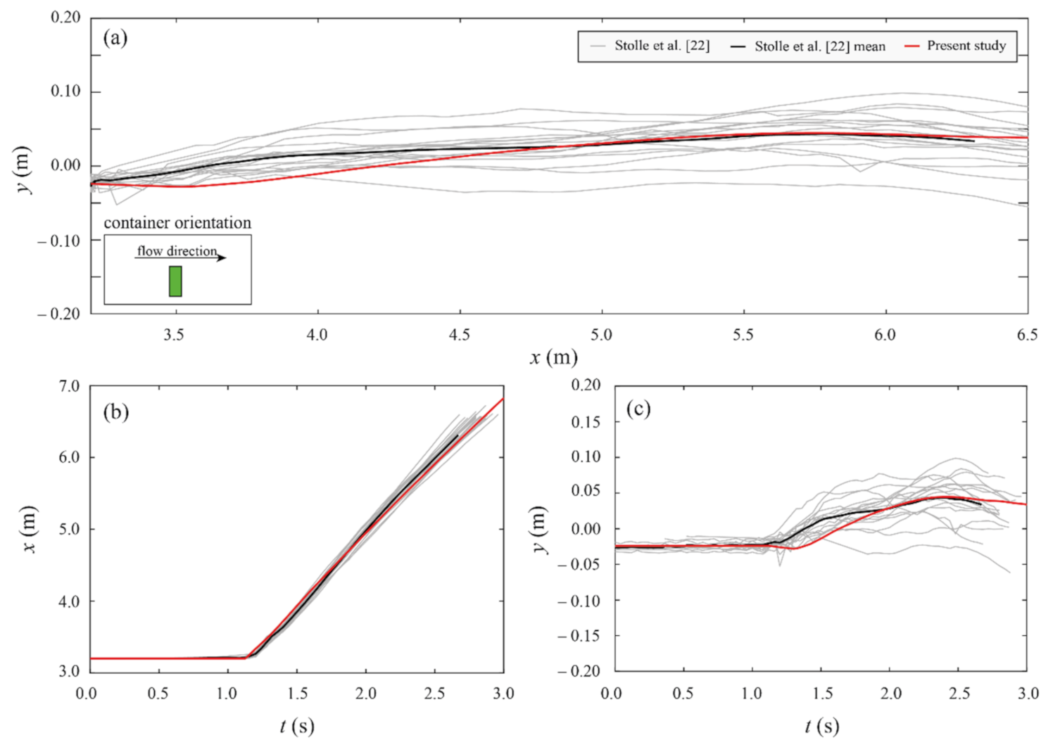
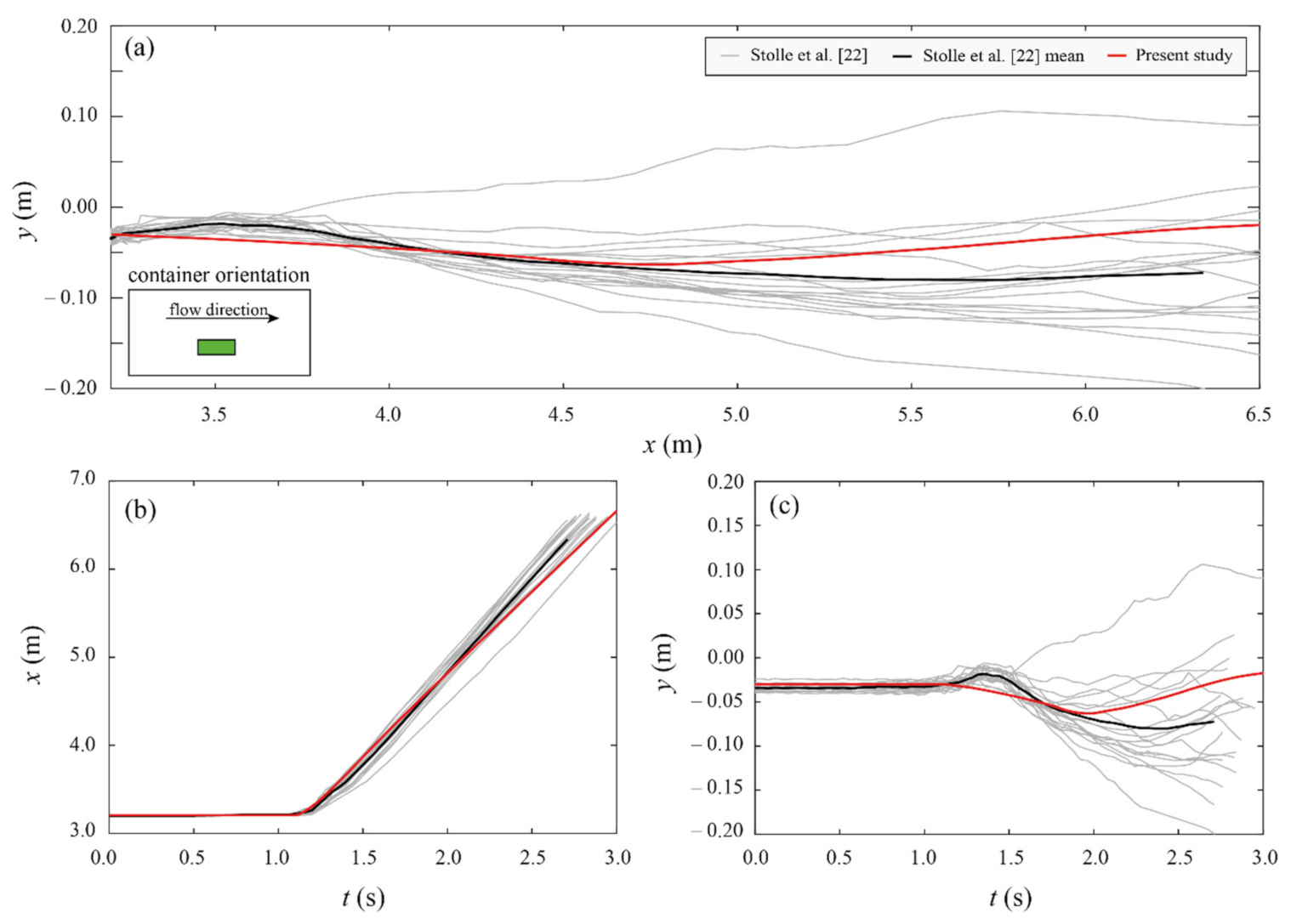
In this section, the container motion is analysed and compared with the experimental findings. Hereafter, only the results with the combination of the material characteristics that gave the most accurate representation of the experiments, after initial calibration, are presented. $K=0.7$ was kept constant for both container and floor whereas a $f_c=0.15$ and $f_c=0.30$ was used for container and floor, respectively. Both OR1 and OR2 container orientations are presented. Only the results of trajectories projected on the x-y plane are shown as the objective of the paper is to validate the simulations with experiments focused on the container motion on a coastal area.

3.3.1. Trajectories

First, the container trajectories are analysed for both OR1 and OR2. Figure 5 illustrates the results for OR1 with Figure 5a showing the trajectory over the test area with the solid grey lines and solid black line representing all the experiments and their mean, respectively, compared with the numerical results represented with a solid red line. Note that the mean experimental values were calculated only up to when data was available for all experimental runs (see Figure 5b). The larger differences between the simulation and the experiments are found during the initial movement, for $x\le 3.5$ m, where the simulated container proceeds almost in a straight line in contrast to the real ones which are very often characterised by a transversal motion as shown also by the mean trajectory. However, at a later stage the simulated container also starts a meandering motion reaching a maximum value of $y=+0.0447$ m at $x=5.77$ m, slightly further than the experimental one for which the same value occurs at $x=5.80$ m. This behaviour of the container can be mainly associated with the not perfectly symmetrical distribution of the masses (Section 2.3) as the flow was mainly symmetrical with respect to the $y$-coordinate in the experiment (see Derschum et al. [20]) as well as in the numerical simulation.

Figure 5b,c show the evolution of the trajectories components in $x$ and $y$, respectively, over time. This helps to additionally identify the point of motion initiation which, although starting slightly before than in the experimental mean due to the slightly higher velocity of the flow, closely matches between simulations and experiments. In Figure 5b it can be noticed that the slope of the $x \left(t\right)$ curve is nearly constant in the simulations, while in the experiments it varies, indicating differences in the velocity as discussed in the next subsection. The performance was measured with the $nRMS{E}_l$, i.e., Equation (7) for both directions and summarised in

Table 3. $nRMS{E}_l$ values OR1 container trajectory.

	$\mathit{x}$	$\mathit{y}$
$nRMS{E}_l$	0.122	0.024

.

The results for OR2 are shown in Figure 6 and compared with the corresponding experiments, as done for OR1. The numerical trajectory (Figure 6a) follows the mean experimental trajectory but with a divergence from the mean values on the $y$-coordinate for $x>4.5$ m. Additionally, the numerical model is not able to reproduce the experimental container trajectory at the onset of the motion, first towards and then away from the centre of the flume. These differences, which are particularly noticeable in Figure 6c, also affect the $nRMS{E}_l$ (

Table 4. $nRMS{E}_l$ values for OR2 container trajectory.

	$\mathit{x}$	$\mathit{y}$
$nRMS{E}_l$	0.190	0.044

) in $y$-direction with a higher value than that for OR1.

3.3.2. Velocity

Hereafter, the velocity of the centroid of the container is analysed to give a deeper insight into the accuracy of the used numerical method in simulating debris motion. As velocities were not directly measured in the laboratory, in this study they were calculated as the time derivative of the trajectory in both x and y directions. The performance of the modelling of the velocity was assess using Equation (8) and the results are shown in

Table 5. $nRMS{E}_v$ values for containers in both initial orientations tested.

Container Orientation	$\mathit{x}$	$\mathit{y}$
OR1	0.135	0.016
OR2	0.133	0.024

. Figure 7a,b shows the container velocity in $x$- ($v_x$) and $y$-directions ($v_y$) for OR1 whereas Figure 7c,d show the results for OR2. The velocity results are more accurate for OR1 than for OR2, even if slightly, as shown in Table 5. Here, the initial container $v_x$ increases almost instantly, probably also due to the deeper tip of the flow, contrarily to the more gradual increase measured in the experiments affecting its motion initiation. However, the final simulated velocity follows closely the experiments with only a relative difference of −4.0% with respect to the experimental value. The opposite is shown for OR2 (Figure 7c) where the gradual $v_x$ increase is similar to the experimental one, but the final velocity results in a larger relative difference of −9.8%, again with respect to the experimental value. Finally, $v_y$ shown in Figure 7d confirms what shown in Section 3.3.1 with an initially negative $v_y$ becoming positive at $t=$1.5 s in the experiments, not being captured by the numerical model where a positive $v_y$ is always computed. Finally, $v_y$ for both cases tends to be more accurately predicted after the container stabilisation with the flow, which occurrs after some time from its initial mobilisation.

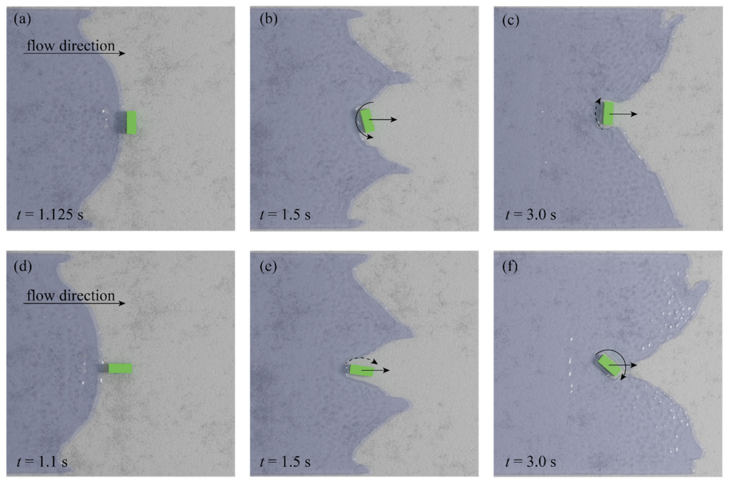
3.3.3. Qualitative Description of the Interaction between Container and Flow

A visualisation of the interaction between flow and container is shown for OR1 and OR2, simulated using the validated model, to qualitatively highlight the key differences of the two orientations. Figure 8 shows a top-down representation of different instants during the simulation.

For OR1 the dam break flow impacts right after $t=1.125$ s (Figure 8a). The interaction after the initial impact starts to develop and, as shown for $t=1.5$ s (Figure 8b), the container starts to rotate counterclockwise due to its eccentricity while the adjacent flow moves faster than the container creating a “u” shape around it. Afterwards, the flow and the container movements start to stabilise (Figure 8c, $t=3.0$ s). Here, the flow starts to close around the container, which rotates slightly clockwise while transported. Note that these rotations affect the transversal trajectory of the container and, in turn, the symmetry and flow direction of the tip of the dam break.

Some differences are found when analysing the interaction between flow and container for OR2. The main difference with OR1 is that, due to the smaller impact area, the flow forms a “v” shape separating from both sides of the container. The container still rotates clockwise, starting slowly at around t = 1.5 s (Figure 8e) but continues to increase with its motion up to $t=3.0$ s instead of changing direction as seen in OR1. Contrarily to what happens for OR1, due to the slightly slower container $v_x$ and different orientation, the dam break flow manages to close around the front part of the container more quickly (Figure 8f).

4. Discussion and Conclusions

This section discusses the findings of this study with the focus on analysing the future applicability of this numerical methodology in a broader context, as introduced in Section 1. First, the accuracy of the simulation results was compared with the accuracy reached by the container experimental measurement system as additional benchmark. Stolle et al. [22], as measurement system, employed an optical tracking algorithm introduced in Stolle et al. [57] where it is investigated its accuracy using the parameters introduced in Section 2.5. The mean values of the parameters calculated by Stolle et al. [57] for the experimental validation tests with a single container are summarised in

Table 6. Accuracy metrics for the smart debris of Stolle et al. [57] and for the numerical simulations of the present study against experimental mean values of Stolle et al. [22].

	$\left|\mathbf{M}{\mathbf{E}}_{\mathit{x}}\right|$	$\left|\mathbf{M}{\mathbf{E}}_{\mathbf{y}}\right|$	$\mathbf{M}\mathbf{D}\mathbf{E}$
Stolle et al. [57]	0.004	0.018	0.023
OR1	0.005	0.004	0.037
OR2	0.014	0.008	0.061

. $\left|\mathrm{ME}\right|$ and $\mathrm{MDE}$ values for the simulations of the present study are additionally calculated for both OR1 and OR2. This helps to highlight the very similar accuracy of the present numerical model and the experimental tracking system in the description of the container trajectory giving further confidence on the employed numerical method.

In conclusion, the coupled models DualSPHysics and CHRONO can accurately simulate the behaviour of a debris transported by a dam break flow. Note that the modelling accuracy is referred to the mean trajectory among the ones resulting from repetitions of the experiment. This is because the numerical model was calibrated using the mean flow and container kinematic conditions, which was necessary given the highly variable characteristics of this phenomenon. Additionally, the calibration process of the model has shown that the details of the container internal structure and, above all, mass distribution is essential to achieve accuracy due to the importance of the container rotation in its kinematics. This rotation is, in fact, responsible for the container drift from the flume axis as in its absence the container would otherwise follow an almost one-dimensional trajectory. The difference in drift from the flume axis between simulations and experiments during the initial stage of the container motion, in turn affecting the velocity, suggests a lower accuracy in the forces if an impact would occur during this stage. However, as the trajectory stabilises the accuracy significantly improves especially for OR1. This has important consequences in modelling the impact of these debris on structures, which is the natural next step of this investigation. It is expected that impact forces are more accurately predicted if the impact occurs at later stages of the transport.

References

1. Mori, N.; Takahashi, T.; Yasuda, T.; Yanagisawa, H. Survey of 2011 Tohoku earthquake tsunami inundation and run-up. Geophys. Res. Lett. 2011, 38, L00G14. [Google Scholar] [CrossRef]
2. Sassa, S.; Takagawa, T. Liquefied gravity flow-induced tsunami: First evidence and comparison from the 2018 Indonesia Sulawesi earthquake and tsunami disasters. Landslides 2019, 16, 195–200. [Google Scholar] [CrossRef] [Green Version]
3. Bellotti, G.; Briganti, R.; Beltrami, G.M. The combined role of bay and shelf modes in tsunami amplification along the coast. J. Geophys. Res. Oceans 2012, 117, C08027. [Google Scholar] [CrossRef]
4. De Girolamo, P.; Di Risio, M.; Romano, A.; Molfetta, M.G. Landslide Tsunami: Physical Modeling for the Implementation of Tsunami Early Warning Systems in the Mediterranean Sea. Procedia Eng. 2014, 70, 429–438. [Google Scholar] [CrossRef] [Green Version]
5. Romano, A.; Di Risio, M.; Bellotti, G.; Molfetta, M.G.; Damiani, L.; De Girolamo, P. Tsunamis generated by landslides at the coast of conical islands: Experimental benchmark dataset for mathematical model validation. Landslides 2016, 13, 1379–1393. [Google Scholar] [CrossRef]
6. Romano, A.; Lara, J.L.; Barajas, G.; Di Paolo, B.; Bellotti, G.; Di Risio, M.; Losada, I.J.; De Girolamo, P. Tsunamis Generated by Submerged Landslides: Numerical Analysis of the Near-Field Wave Characteristics. J. Geophys. Res. Oceans 2020, 125, e2020JC016157. [Google Scholar] [CrossRef]
7. Ruffini, G.; Heller, V.; Briganti, R. Numerical characterisation and efficient prediction of landslide-tsunami propagation over a wide range of idealised bathymetries. Coast. Eng. 2021, 103854, in press. [Google Scholar] [CrossRef]
8. Naito, C.; Cercone, C.; Riggs, H.R.; Cox, D. Procedure for Site Assessment of the Potential for Tsunami Debris Impact. J. Waterw. Port Coast. Ocean Eng. 2014, 140, 223–232. [Google Scholar] [CrossRef]
9. FEMA. P646 Guidelines for Design of Structure for Vertical Evacuation from Tsunamis; Federal Emergency Management Agency: Redwood City, CA, USA, 2012. [Google Scholar]
10. Haehnel, R.B.; Daly, S.F. Maximum impact force of woody debris on flood plain structures. J. Hydraul. Eng. 2004, 130, 112–120. [Google Scholar] [CrossRef]
11. American Society for Civil Engineers (ASCE). Minimum Design Loads and Associated Criteria for Buildings and Other Structures; ASCE/SEI 7-16; American Society for Civil Engineers (ASCE): Reston, VA, USA, 2016. [Google Scholar]
12. Imamura, F.; Goto, K.; Ohkubo, S. A numerical model for the transport of a boulder by tsunami. J. Geophys. Res. Space Phys. 2008, 113, C01008. [Google Scholar] [CrossRef]
13. Rueben, M.; Cox, D.; Holman, R.; Shin, S.; Stanley, J. Optical Measurements of Tsunami Inundation and Debris Movement in a Large-Scale Wave Basin. J. Waterw. Port Coast. Ocean Eng. 2015, 141, 04014029. [Google Scholar] [CrossRef]
14. Goseberg, N.; Stolle, J.; Nistor, I.; Shibayama, T. Experimental analysis of debris motion due the obstruction from fixed obstacles in tsunami-like flow conditions. Coast. Eng. 2016, 118, 35–49. [Google Scholar] [CrossRef]
15. Nistor, I.; Goseberg, N.; Stolle, J.; Mikami, T.; Shibayama, T.; Nakamura, R.; Matsuba, S. Experimental Investigations of Debris Dynamics over a Horizontal Plane. J. Waterw. Port Coast. Ocean Eng. 2017, 143, 04016022. [Google Scholar] [CrossRef]
16. Nouri, Y.; Nistor, I.; Palermo, D.; Cornett, A. Experimental Investigation of Tsunami Impact on Free Standing Structures. Coast. Eng. J. 2010, 52, 43–70. [Google Scholar] [CrossRef]
17. Riggs, H.R.; Cox, D.T.; Naito, C.J.; Kobayashi, M.H.; Piran Aghl, P.; Ko, H.S.; Khowitar, E. Experimental and analytical study of water-driven debris impact forces on structures. J. Offshore Mech. Arct. Eng. 2014, 136, 041603. [Google Scholar] [CrossRef]
18. Ikeno, M.; Takabatake, D.; Kihara, N.; Kaida, H.; Miyagawa, Y.; Shibayama, A. Improvement of collision force formula for woody debris by airborne and hydraulic experiments. Coast. Eng. J. 2016, 58, 1640022. [Google Scholar] [CrossRef] [Green Version]
19. Shafiei, S.; Melville, B.W.; Shamseldin, A.Y.; Beskhyroun, S.; Adams, K.N. Measurements of tsunami-borne debris impact on structures using an embedded accelerometer. J. Hydraul. Res. 2016, 54, 435–449. [Google Scholar] [CrossRef]
20. Derschum, C.; Nistor, I.; Stolle, J.; Goseberg, N. Debris impact under extreme hydrodynamic conditions part 1: Hydrodynamics and impact geometry. Coast. Eng. 2018, 141, 24–35. [Google Scholar] [CrossRef]
21. Stolle, J.; Derschum, C.; Goseberg, N.; Nistor, I.; Petriu, E. Debris impact under extreme hydrodynamic conditions part 2: Impact force responses for non-rigid debris collisions. Coast. Eng. 2018, 141, 107–118. [Google Scholar] [CrossRef]
22. Stolle, J.; Goseberg, N.; Nistor, I.; Petriu, E. Probabilistic Investigation and Risk Assessment of Debris Transport in Extreme Hydrodynamic Conditions. J. Waterw. Port Coast. Ocean Eng. 2018, 144, 04017039. [Google Scholar] [CrossRef]
23. Goseberg, N.; Nistor, I.; Mikami, T.; Shibayama, T.; Stolle, J. Nonintrusive Spatiotemporal Smart Debris Tracking in Turbulent Flows with Application to Debris-Laden Tsunami Inundation. J. Hydraul. Eng. 2016, 142, 04016058. [Google Scholar] [CrossRef]
24. Nistor, I.; Goseberg, N.; Stolle, J. Tsunami-Driven Debris Motion and Loads: A Critical Review. Front. Built Environ. 2017, 3, 2. [Google Scholar] [CrossRef] [Green Version]
25. Wu, T.R.; Chu, C.R.; Huang, C.J.; Wang, C.Y.; Chien, S.Y.; Chen, M.Z. A two-way coupled simulation of moving solids in free-surface flows. Comput. Fluids 2014, 100, 347–355. [Google Scholar] [CrossRef]
26. De Finis, S.; Romano, A.; Bellotti, G. Numerical and laboratory analysis of post-overtopping wave impacts on a storm wall for a dike-promenade structure. Coast. Eng. 2020, 155, 103598. [Google Scholar] [CrossRef]
27. Chen, F.; Heller, V.; Briganti, R. Numerical modelling of tsunamis generated by iceberg calving validated with large-scale laboratory experiments. Adv. Water Resour. 2020, 142, 103647. [Google Scholar] [CrossRef]
28. Koshizuka, S.; Oka, Y. Moving-Particle Semi-Implicit Method for Fragmentation of Incompressible Fluid. Nucl. Sci. Eng. 1996, 123, 421–434. [Google Scholar] [CrossRef]
29. Gomez-Gesteira, M.; Rogers, B.D.; Crespo, A.J.C.; Dalrymple, R.A.; Narayanaswamy, M.; Dominguez, J.M. SPHysics–development of a free-surface fluid solver Part 1: Theory and formulations. Comput. Geosci. 2012, 48, 289–299. [Google Scholar] [CrossRef]
30. Koshizuka, S.; Nobe, A.; Oka, Y. Numerical analysis of breaking waves using the moving particle semi-implicit method. Int. J. Numer. Methods Fluids 1998, 26, 751–769. [Google Scholar] [CrossRef]
31. Amicarelli, A.; Albano, R.; Mirauda, D.; Agate, G.; Sole, A.; Guandalini, R. A Smoothed Particle Hydrodynamics model for 3D solid body transport in free surface flows. Comput. Fluids 2015, 116, 205–228. [Google Scholar] [CrossRef]
32. Tan, H.; Ruffini, G.; Heller, V.; Chen, S. A Numerical Landslide-Tsunami Hazard Assessment Technique Applied on Hypothetical Scenarios at Es Vedrà, Offshore Ibiza. J. Mar. Sci. Eng. 2018, 6, 111. [Google Scholar] [CrossRef] [Green Version]
33. Heller, V.; Bruggemann, M.; Spinneken, J.; Rogers, B.D. Composite modelling of subaerial landslide–tsunamis in different water body geometries and novel insight into slide and wave kinematics. Coast. Eng. 2016, 109, 20–41. [Google Scholar] [CrossRef]
34. Rogers, B.D.; Dalrymple, R.A.; Stansby, P.K.; Smith, J.M. SPH modeling of floating bodies in the surf zone. In Coastal Engineering 2008: (In 5 Volumes); World Scientific Publishing Co Pte Lt: Singapore, 2009; pp. 204–215. [Google Scholar]
35. Canelas, R.; Ferreira, R.M.; Crespo, A.; Domínguez, J.M. A generalized SPH-DEM discretization for the modelling of complex multiphasic free surface flows. In Proceedings of the 8th International SPHERIC Workshop, Trondheim, Norway, 4–6 June 2013; pp. 74–79. [Google Scholar]
36. Canelas, R.B.; Domínguez, J.M.; Crespo, A.J.; Gómez-Gesteira, M.; Ferreira, R.M. A smooth particle hydrodynamics discretization for the modelling of free surface flows and rigid body dynamics. Int. J. Numer. Methods Fluids 2015, 78, 581–593. [Google Scholar] [CrossRef]
37. Goseberg, N.; Heunecke, M.; Stolle, J.; Nistor, I. Numerical modelling of shipping container transport over horizontal bottom. In Proceedings of the International Short Course and Conference on Applied Coastal Research, Santander, Spain, 3–6 October 2017. [Google Scholar]
38. Crespo, A.J.C.; Domínguez, J.M.; Rogers, B.D.; Gómez-Gesteira, M.; Longshaw, S.; Canelas, R.; Vacondio, R.; Barreiro, A.; García-Feal, O. DualSPHysics: Open-source parallel CFD solver based on Smoothed Particle Hydrodynamics (SPH). Comput. Phys. Commun. 2015, 187, 204–216. [Google Scholar] [CrossRef]
39. Domínguez, J.M.; Fourtakas, G.; Altomare, C.; Canelas, R.B.; Tafuni, A.; García-Feal, O.; Martínez-Estévez, I.; Mokos, A.; Vacondio, R.; Crespo, A.J.C.; et al. DualSPHysics: From fluid dynamics to Multiphysics problems. Comput. Part Mech. 2021, 1–29. [Google Scholar] [CrossRef]
40. Tasora, A.; Anitescu, M. A matrix-free cone complementarity approach for solving large-scale, nonsmooth, rigid body dynamics. Comput. Methods Appl. Mech. Eng. 2011, 200, 439–453. [Google Scholar] [CrossRef] [Green Version]
41. Anitescu, M.; Tasora, A. An iterative approach for cone complementarity problems for nonsmooth dynamics. Comput. Optim. Appl. 2010, 47, 207–235. [Google Scholar] [CrossRef]
42. Tagliafierro, B.; Mancini, S.; Ropero-Giralda, P.; Domínguez, J.M.; Crespo, A.J.C.; Viccione, G. Performance Assessment of a Planing Hull Using the Smoothed Particle Hydrodynamics Method. J. Mar. Sci. Eng. 2021, 9, 244. [Google Scholar] [CrossRef]
43. Violeau, D.; Rogers, B.D. Smoothed particle hydrodynamics (SPH) for free-surface flows: Past, present and future. J. Hydraul. Res. 2016, 54, 1–26. [Google Scholar] [CrossRef]
44. Monaghan, J.J. Smoothed particle hydrodynamics. Annu. Rev. Astron. Astrophys. 1992, 30, 543–574. [Google Scholar] [CrossRef]
45. Gotoh, H.; Shao, S.; Memita, T. SPH-LES model for numerical investigation of wave interaction with partially immersed breakwater. Coast. Eng. J. 2001, 46, 39–63. [Google Scholar] [CrossRef]
46. Liu, G.R.; Liu, M.B. Smoothed Particle Hydrodynamics: A Meshfree Particle Method; World Scientific Publishing Co Pte Lt: Singapore, 2003. [Google Scholar]
47. Crespo, A.J.C.; Gómez-Gesteira, M.; Dalrymple, R.A. Boundary conditions generated by dynamic particles in SPH methods. Comput. Mater. Contin. 2007, 5, 173–184. [Google Scholar]
48. Gomez-Gesteira, M.; Rogers, B.D.; Dalrymple, R.A.; Crespo, A.J. State-of-the-art of classical SPH for free-surface flows. J. Hydraul. Res. 2010, 48, 6–27. [Google Scholar] [CrossRef]
49. Stolle, J.; Ghodoosipour, B.; Derschum, C.; Nistor, I.; Petriu, E.; Goseberg, N. Swing gate generated dam-break waves. J. Hydraul. Res. 2019, 57, 675–687. [Google Scholar] [CrossRef]
50. Wendland, H. Piecewise polynomial, positive definite and compactly supported radial functions of minimal degree. Adv. Comput. Math. 1995, 4, 389–396. [Google Scholar] [CrossRef]
51. Fourtakas, G.; Vacondio, R.; Domínguez, J.M.; Rogers, B.D. Improved density diffusion term for long duration wave propagation. In Proceedings of the International SPHERIC Workshop, Harbin, China, 13–16 January 2020. [Google Scholar]
52. Tan, H.; Xu, Q.; Chen, S. Subaerial rigid landslide-tsunamis: Insights from a block DEM-SPH model. Eng. Anal. Bound. Elem. 2018, 95, 297–314. [Google Scholar] [CrossRef]
53. Vacondio, R.; Mignosa, P.; Pagani, S. 3D SPH numerical simulation of the wave generated by the Vajont rockslide. Adv. Water Resour. 2013, 59, 146–156. [Google Scholar] [CrossRef]
54. Harper, C.A. Modern Plastics Handbook; McGraw Hill Professional: New York, NY, USA, 2000. [Google Scholar]
55. Michael, L.B. SPI Plastics Engineering Handbook of the Society of the Plastics Industry; Springer: New York, NY, USA, 1991. [Google Scholar]
56. Stolle, J.; Nistor, I.; Goseberg, N. Optical Tracking of Floating Shipping Containers in a High-Velocity Flow. Coast. Eng. J. 2016, 58, 1650005. [Google Scholar] [CrossRef]
57. Stolle, J.; Nistor, I.; Goseberg, N.; Petriu, E. Multiple Debris Impact Loads in Extreme Hydrodynamic Conditions. J. Waterw. Port Coast. Ocean Eng. 2020, 146, 04019038. [Google Scholar] [CrossRef]
58. Chanson, H. Tsunami Surges on Dry Coastal Plains: Application of Dam Break Wave Equations. Coast. Eng. J. 2006, 48, 355–370. [Google Scholar] [CrossRef] [Green Version]
Figure 1. Numerical domain in (a) 3D view and (b) top view for OR1.
Applsci 11 03618 g001
Figure 2. 3D modelled container for high resolution “container only” simulation.
Applsci 11 03618 g002
Figure 3. Comparison of h / h 0 between numerical results and Stolle et al. [21] at (a) WG1 ( n R M S E l = 0.010 ), (b) WG2 ( n R M S E l = 0.068 ) and (c) WG3 ( n R M S E l = 0.031 ).
Applsci 11 03618 g003
Figure 4. Comparison of Δ x and Δ y to analyse the effects of (a,b) f c and (c,d) K on container dynamics.
Applsci 11 03618 g004
Figure 5. Comparison between experimental and numerical results: (a) trajectories and their time evolution in (b) x and (c) y directions for OR1.
Applsci 11 03618 g005
Figure 6. Comparison between experimental and numerical results: (a) trajectories and their time evolution in (b) x and (c) y directions for OR2.
Applsci 11 03618 g006
Figure 7. Comparison between experimental and numerical container velocities v x and v y for (a,b) OR1 and (c,d) OR2.
Applsci 11 03618 g007
Figure 8. Qualitative comparison of the flow debris interaction between (ac) OR1 and (df) OR2.
Applsci 11 03618 g008