
Tree Internal Defected Imaging Using Model-Driven Deep Learning Network


Abstract
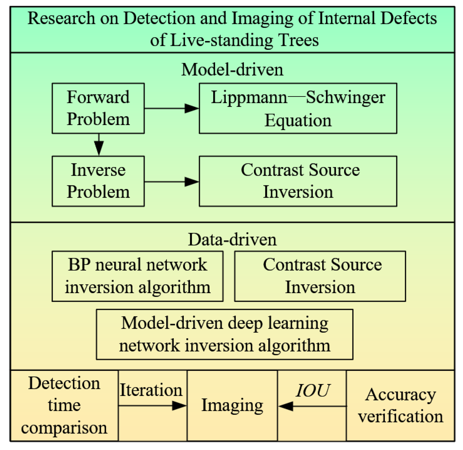
:1. Introduction
- The objective function of the comparison source inversion is obtained by using the Lippmann–Schwinger equation and the equivalent current source radiation process of the scattering field. The models of comparison; source inversion algorithm, BP neural network inversion algorithm, and model-driven inversion algorithm based on deep learning networks, are established;
- Determine the simulated imaging evaluation metrics; on the basis of building simulation environment and training database, the inversion imaging of single defect, homogeneous double defect and heterogeneous multi-defect is realized, and the algorithm iterative stability is analyzed.
2. Method
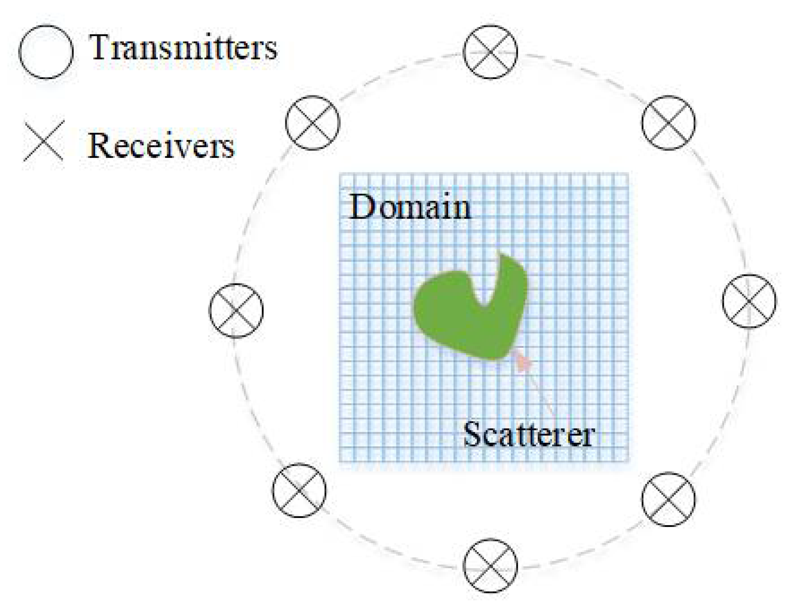
2.1. Scattering Problem
2.2. Contrast Source Inversion (CSI) Method
2.3. BP Neural Network Inversion Algorithm
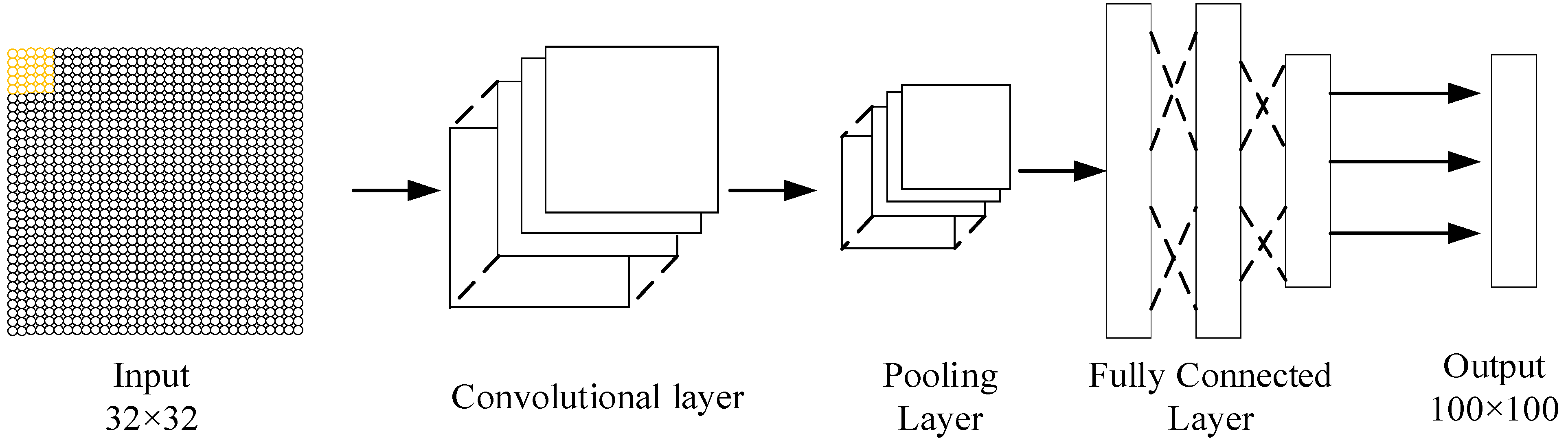
2.4. Model-Driven Inversion Algorithm Based on Deep Learning Networks
3. Experimental Results and Analysis
3.1. Simulated Imaging Evaluation Metrics
3.1.1. Intersection over Union
3.1.2. Algorithm Detection Accuracy
3.2. Model Settings
3.2.1. Build Simulation Environment
3.2.2. Build Training Database
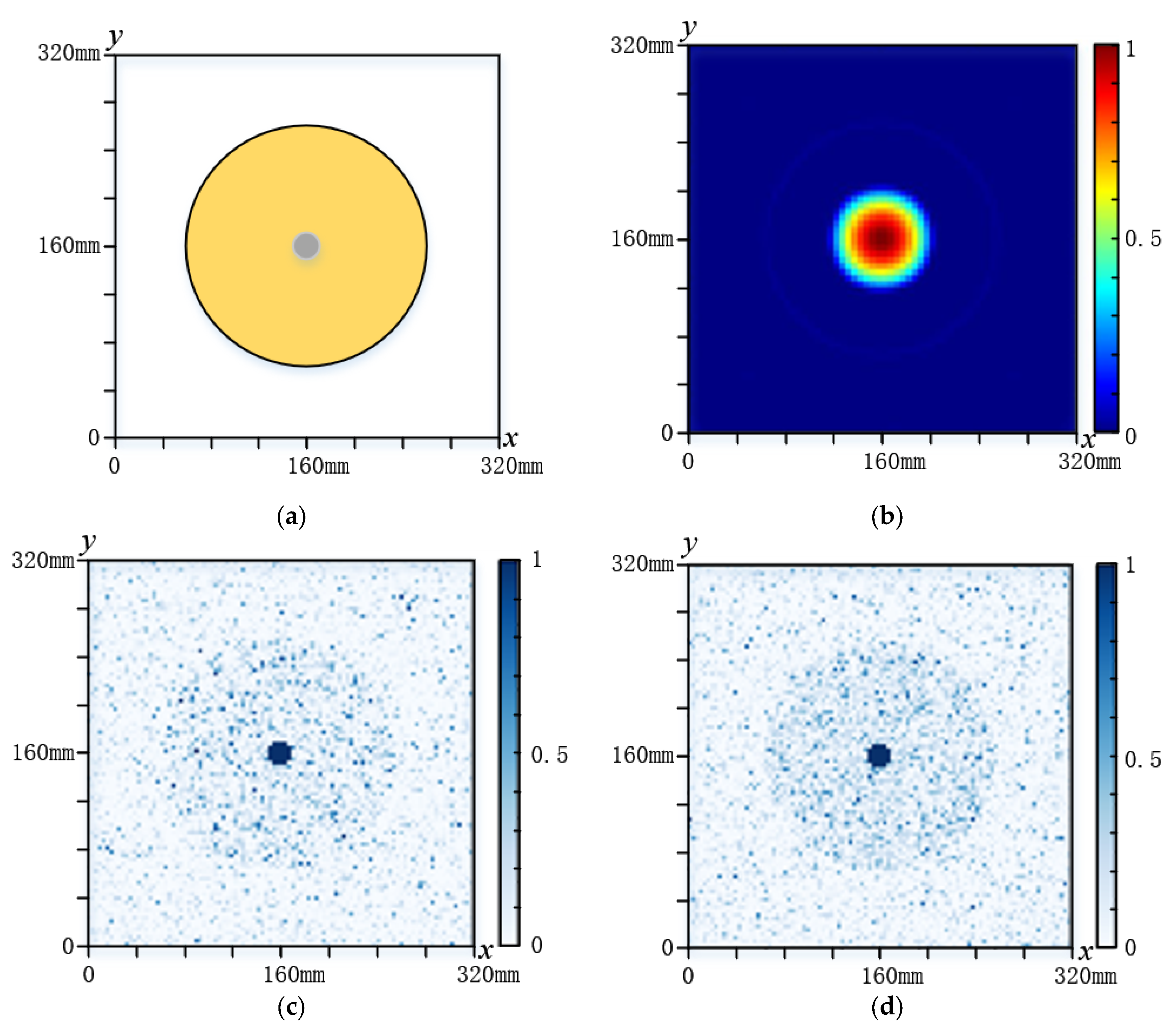
3.3. Single Defect Inverse Imaging
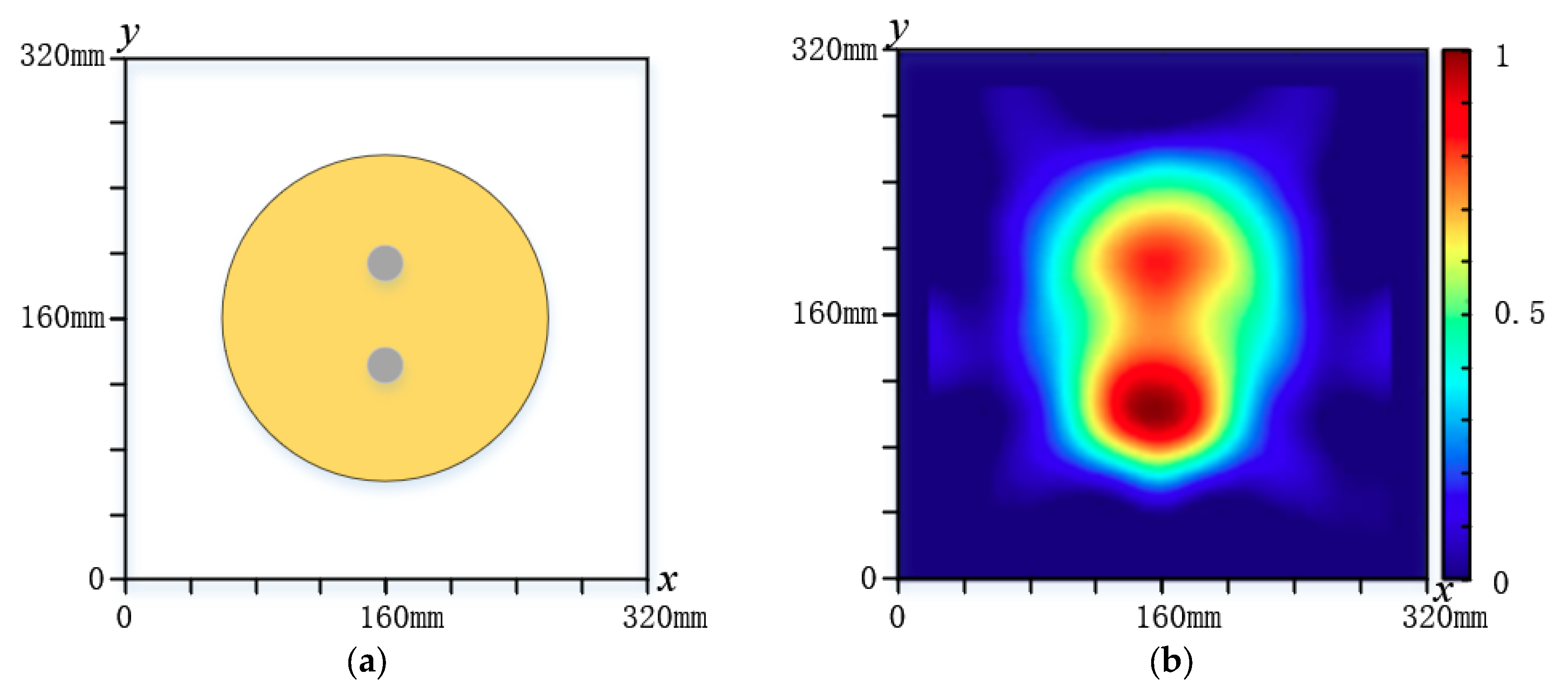
3.4. Homogeneous Double Defect Inversion Imaging
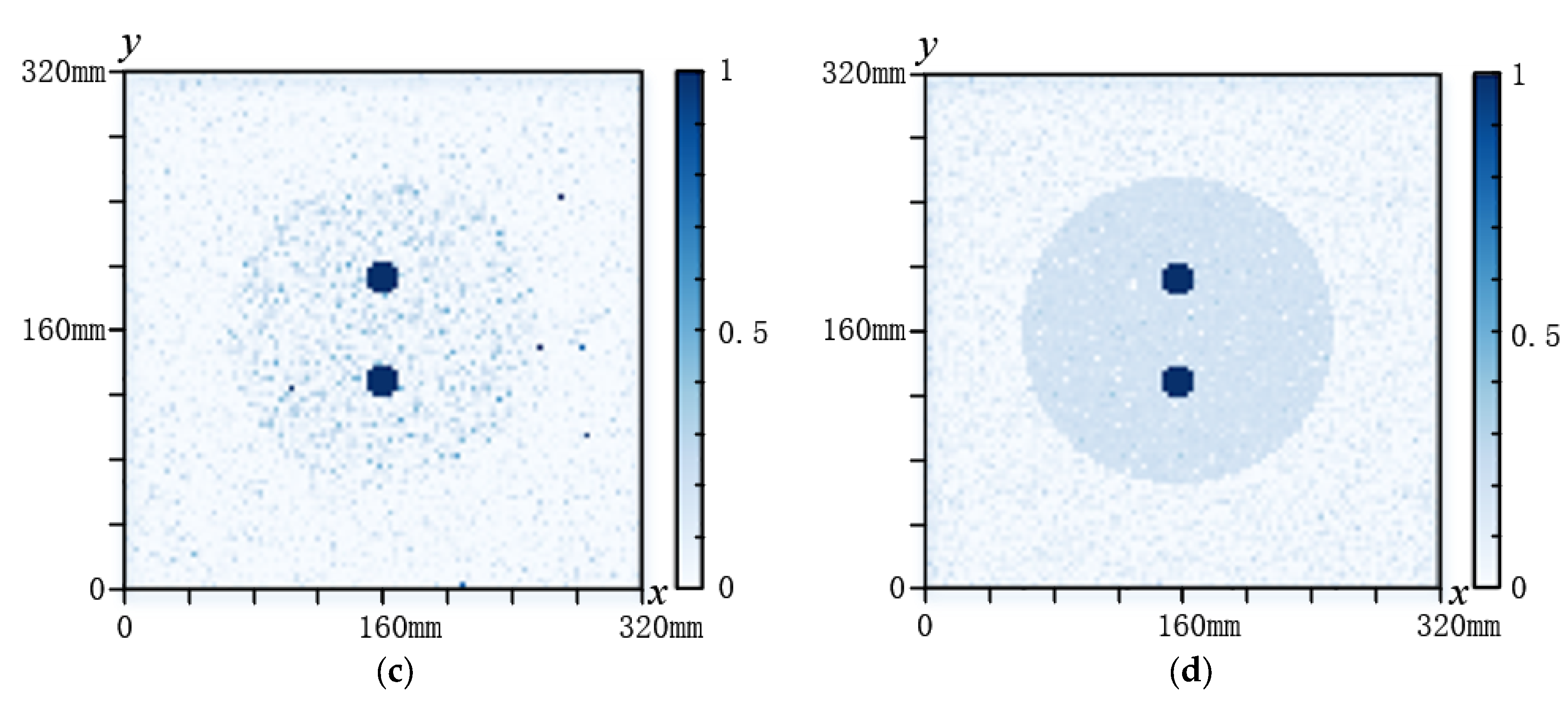
3.5. Heterogeneous Multi-Defect Inversion Imaging
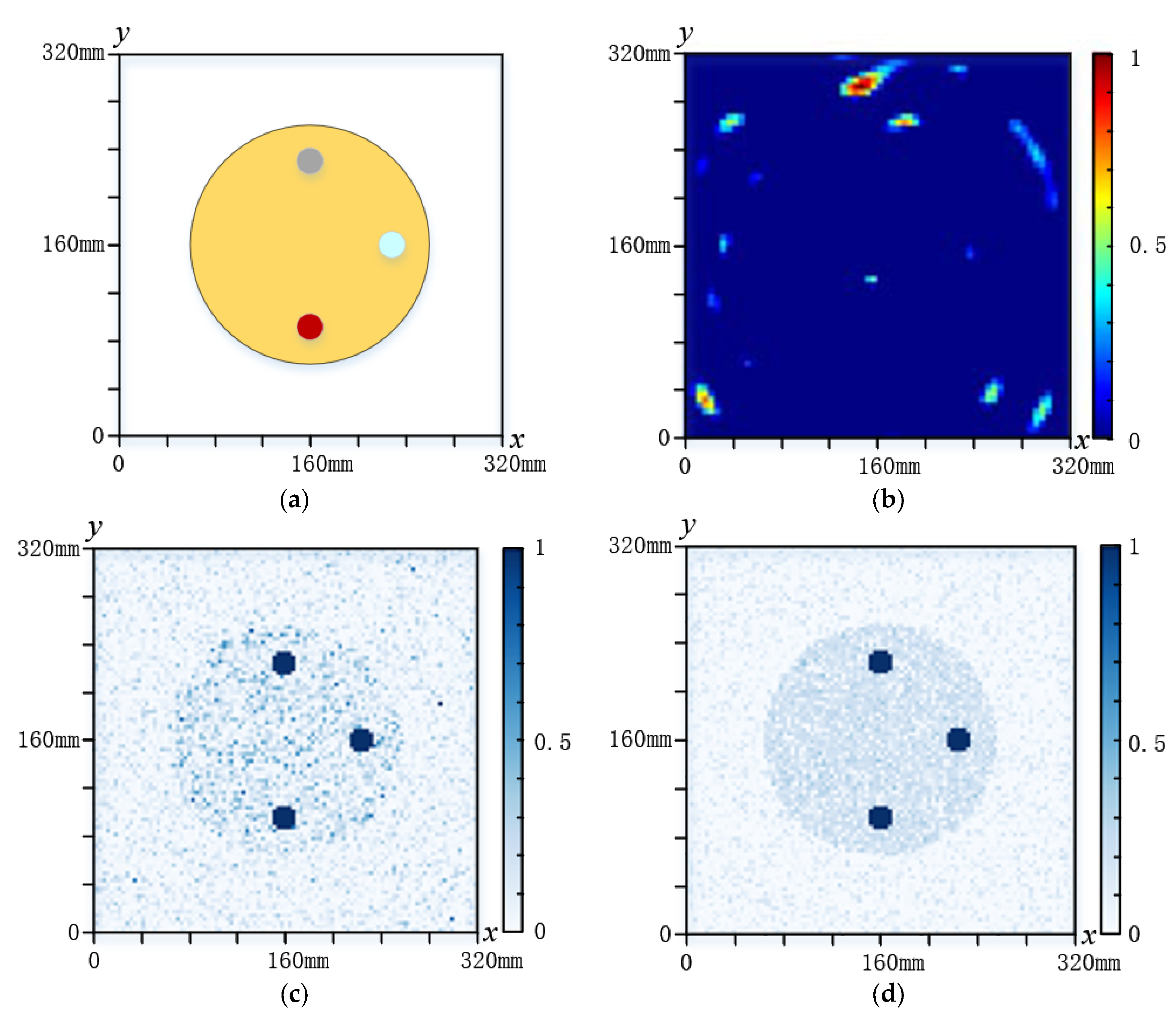
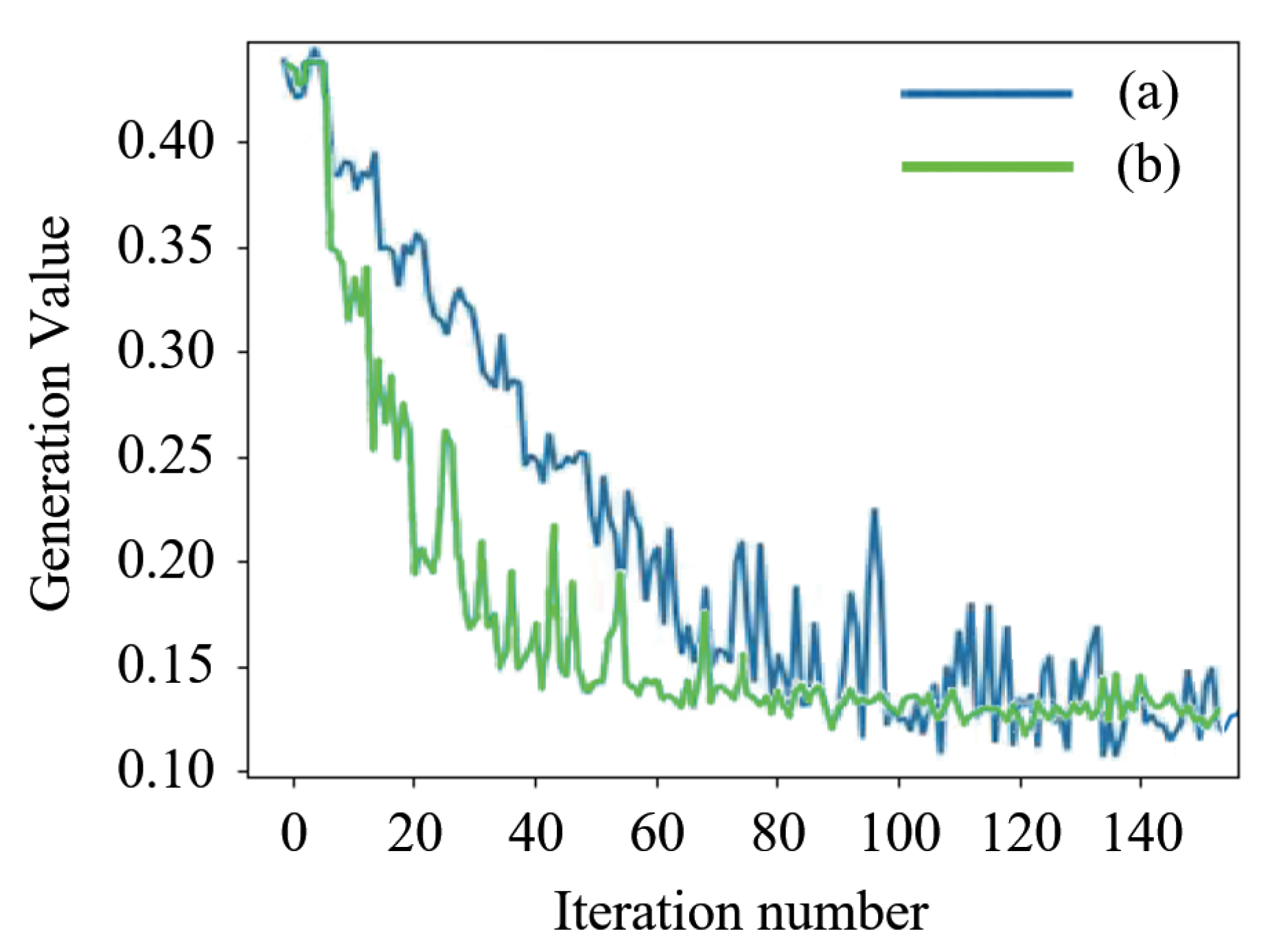
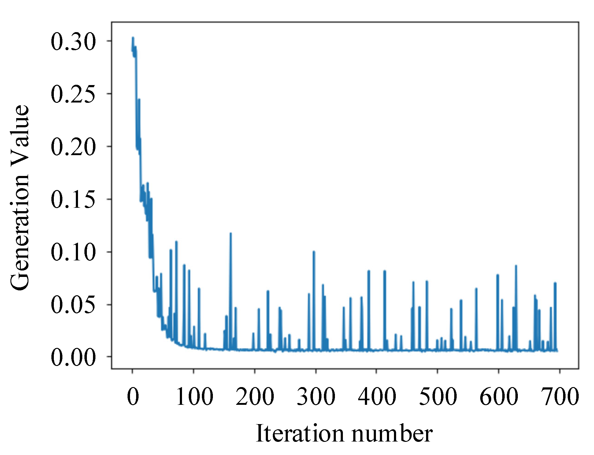
3.6. Algorithm Iterative Stability Analysis
4. Conclusions
Author Contributions
Funding
Institutional Review Board Statement
Informed Consent Statement
Data Availability Statement
Conflicts of Interest
References
- Ayanleye, S.; Nasir, V.; Avramidis, S.; Cool, J. Effect of wood surface roughness on prediction of structural timber properties by infrared spectroscopy using ANFIS, ANN and PLS regression. Eur. J. Wood Wood Prod. 2021, 79, 101–115. [Google Scholar] [CrossRef]
- Du, X.C.; Li, J.J.; Feng, H.L.; Chen, S.Y. Image Reconstruction of Internal Defects in Wood Based on Segmented Propagation Rays of Stress Waves. Appl. Sci. 2018, 8, 1778. [Google Scholar] [CrossRef] [Green Version]
- Jezova, J.; Mertens, L.; Lambot, S. Ground-penetrating radar for Observing tree trunks and other cylindrical objects. Constr. Build. Mater. 2016, 123, 214–225. [Google Scholar] [CrossRef]
- Zang, G.S.; Sun, L.J.; Chen, Z.; Li, L. A nondestructive evaluation method for semi-rigid base cracking condition of asphalt pavement. Constr. Build. Mater. 2018, 162, 892–897. [Google Scholar] [CrossRef]
- Yang, Y.T.; Zhou, X.L.; Liu, Y.; Hu, Z.K.; Ding, F.L. Wood Defect Detection Based on Depth Extreme Learning Machine. Appl. Sci. 2020, 10, 7488. [Google Scholar] [CrossRef]
- Yin, Q.; Liu, H.H. Drying Stress and Strain of Wood: A Review. Appl. Sci. 2021, 11, 5023. [Google Scholar] [CrossRef]
- Ji, B.P.; Zhang, Q.D.; Cao, J.S.; Zhang, B.Y.; Zhang, L.Y. Delamination Detection in Bimetallic Composite Using Laser Ultrasonic Bulk Waves. Appl. Sci. 2017, 11, 636. [Google Scholar] [CrossRef]
- Lee, I.S.; Lee, J.W. Nondestructive Internal Defect Detection Using a CW-THz Imaging System in XLPE for Power Cable Insulation. Appl. Sci. 2020, 10, 2055. [Google Scholar] [CrossRef] [Green Version]
- Du, X.; Li, S.; Li, G.; Feng, H.; Chen, S. Stress Wave Tomography of Wood Internal Defects using Ellipse-Based Spatial Interpolation and Velocity Compensation. Bioresources 2015, 10, 3948–3962. [Google Scholar] [CrossRef]
- Taskhiri, M.S.; Hafezi, M.H.; Harle, R.; Williams, D.; Kundu, T.; Turner, P. Ultrasonic and thermal testing to non-destructively identify internal defects in plantation eucalypts. Comput. Electron. Agric. 2020, 173, 105396. [Google Scholar] [CrossRef]
- Du, X.; Feng, H.; Hu, M.; Fang, Y.; Chen, S. Three-dimensional stress wave imaging of wood internal defects using TKriging method. Comput. Electron. Agric. 2018, 148, 63–71. [Google Scholar] [CrossRef]
- Mousavi, M.; Taskhiri, M.S.; Holloway, D.; Olivier, J.C.; Turner, P. Feature extraction of wood-hole defects using empirical mode decomposition of ultrasonic signals. NDT E Int. 2020, 114, 102282. [Google Scholar] [CrossRef]
- Pan, L.; Rogulin, R.; Kondrashev, S. Artificial neural network for defect detection in CT images of wood. Comput. Electron. Agric. 2021, 187, 106312. [Google Scholar] [CrossRef]
- Ali, E.; Xu, W.; Ding, X. Improved optical image matching time series inversion approach for monitoring dune migration in North Sinai Sand Sea: Algorithm procedure, application, and validation. Isprs J. Photogramm. Remote. Sens. 2020, 164, 106–124. [Google Scholar] [CrossRef]
- Ni, Q.-Q.; Hong, J.; Xu, P.; Xu, Z.; Khvostunkov, K.; Xia, H. Damage detection of CFRP composites by electromagnetic wave nondestructive testing (EMW-NDT). Compos. Sci. Technol. 2021, 210, 108839. [Google Scholar] [CrossRef]
- Wang, H.; Che, A.; Feng, S.; Ge, X. Full waveform inversion applied in defect investigation for ballastless undertrack structure of high-speed railway. Tunn. Undergr. Space Technol. 2016, 51, 202–211. [Google Scholar] [CrossRef]
- Xu, X.Q.; Lu, J.S.; Zhang, N.; Yang, T.C.; He, J.Y.; Yao, X.; Cheng, T.; Zhu, Y.; Cao, W.X.; Tian, Y.C. Inversion of rice canopy chlorophyll content and leaf area index based on coupling of radiative transfer and Bayesian network models. Isprs J. Photogramm. Remote. Sens. 2019, 150, 185–196. [Google Scholar] [CrossRef]
- Wang, Y.; Zhang, W.; Gao, R.; Jin, Z.; Wang, X. Recent advances in the application of deep learning methods to forestry. Wood Sci. Technol. 2021, 55, 1171–1202. [Google Scholar] [CrossRef]
- Arens, T.; Ji, X.; Liu, X. Inverse electromagnetic obstacle scattering problems with multi-frequency sparse backscattering far field data. Inverse Probl. 2020, 36, 105007. [Google Scholar] [CrossRef]
- Svendsen, D.H.; Morales-Alvarez, P.; Belen Ruesca, A.; Molina, R.; Camps-Valls, G. Deep Gaussian processes for biogeophysical parameter retrieval and model inversion. Isprs J. Photogramm. Remote. Sens. 2020, 166, 68–81. [Google Scholar] [CrossRef] [PubMed]
- Schneider, M. Lippmann-Schwinger solvers for the computational homogenization of Mater. with pores. Int. J. Numer. Methods Eng. 2020, 121, 5017–5041. [Google Scholar] [CrossRef]
- Xiong, X.; Xue, X.; Qian, Z. A modified iterative regularization method for ill-posed problems. Appl. Numer. Math. 2017, 122, 108–128. [Google Scholar] [CrossRef]
- Hinton, G.E.; Osindero, S.; Teh, Y.-W. A fast learning algorithm for deep belief nets. Neural Comput. 2006, 18, 1527–1554. [Google Scholar] [CrossRef]
- LeCun, Y.; Bengio, Y.; Hinton, G. Deep learning. Nature 2015, 521, 436–444. [Google Scholar] [CrossRef]
- Fathi, H.; Nasir, V.; Kazemirad, S. Prediction of the mechanical properties of wood using guided wave propagation and machine learning. Constr. Build. Mater. 2020, 262, 120848. [Google Scholar] [CrossRef]
- Onofrey, J.A.; Staib, L.H.; Huang, X.; Zhang, F.; Papademetris, X.; Metaxas, D.; Rueckert, D.; Duncan, J.S. Sparse Data-Driven Learning for Effective and Efficient Biomedical Image Segmentation. Annu. Rev. Biomed. Eng. 2020, 22, 127–153. [Google Scholar] [CrossRef] [Green Version]
- Guo, G.; Zhang, N. A survey on deep learning based face recognition. Comput. Vis. Image Underst. 2019, 189, 102805. [Google Scholar] [CrossRef]
- Hsieh, T.-H.; Kiang, J.-F. Comparison of CNN Algorithms on Hyperspectral Image Classification in Agricultural Lands. Sensors 2020, 20, 1734. [Google Scholar] [CrossRef] [Green Version]
- Xi, Z.; Hopkinson, C.; Rood, S.B.; Peddle, D.R. See the forest and the trees: Effective machine and deep learning algorithms for wood filtering and tree species classification from terrestrial laser scanning. Isprs J. Photogramm. Remote. Sens. 2020, 168, 1–16. [Google Scholar] [CrossRef]
- Adibhatla, V.A.; Chih, H.C.; Hsu, C.; Cheng, J.; Abbod, M.F.; Shieh, J.S. Defect Detection in Printed Circuit Boards Using You-Only-Look-Once Convolutional Neural Networks. Electronics 2020, 9, 1547. [Google Scholar] [CrossRef]
- He, T.; Liu, Y.; Yu, Y.; Zhao, Q.; Hu, Z. Application of deep convolutional neural network on feature extraction and detection of wood defects. Measurement 2020, 152, 107357. [Google Scholar] [CrossRef]
- Wang, B.; Li, Y.; Luo, Y.; Li, X.; Freiheit, T. Early event detection in a deep-learning driven quality prediction model for ultrasonic welding. J. Manuf. Syst. 2021, 60, 325–336. [Google Scholar] [CrossRef]
- Mei, S.; Cai, Q.; Gao, Z.; Hu, H.; Wen, G. Deep Learning Based Automated Inspection of Weak Mi-croscratches in Optical Fiber Connector End-Face. IEEE Trans. Instrum.-Tion Meas. 2021, 70, 1–10. [Google Scholar] [CrossRef]
- Zhang, G.; Pan, Y.; Zhang, L. Semi-supervised learning with GAN for automatic defect detection from images. Autom. Constr. 2021, 128, 103764. [Google Scholar] [CrossRef]
- Kurrant, D.; Baran, A.; LoVetri, J.; Fear, E. Integrating prior information into microwave tomography Part 1: Impact of detail on image quality. Med. Phys. 2017, 44, 6461–6481. [Google Scholar] [CrossRef]
- Zhang, P.; Xue, J.; Lan, C.; Zeng, W.; Gao, Z.; Zheng, N. EleAtt-RNN: Adding Attentiveness to Neurons in Recurrent Neural Networks. IEEE Trans. Image Process. 2020, 29, 1061–1073. [Google Scholar] [CrossRef] [Green Version]
- Ostovar, A.; Talbot, B.; Puliti, S.; Astrup, R.; Ringdahl, O. Detection and Classification of Root and Butt-Rot (RBR) in Stumps of Norway Spruce Using RGB Images and Machine Learning. Sensor 2019, 19, 1579. [Google Scholar] [CrossRef] [Green Version]
- Kamal, K.; Qayyum, R.; Mathavan, S.; Zafar, T. Wood defects classification using laws texture energy measures and supervised learning approach. Adv. Eng. Inform. 2017, 34, 125–135. [Google Scholar] [CrossRef]
- de Andrade, B.G.; Basso, V.M.; de Figueiredo Latorraca, J.V. Machine vision for field-level wood identification. IAWA J. 2020, 41, 681–698. [Google Scholar] [CrossRef]


| Physical Variable | Interpretation | Physical Variable | Interpretation |
|---|---|---|---|
| Total field of electric field | Incident field of electric field | ||
| Scattering field of electric field | Angular frequency | ||
| Air-permeability | Air-permittivity | ||
| Relative permittivity | Wavenumber | ||
| Contrast source | Contrast factor | ||
| Normalization parameter |
| Parameter Name | Value | Parameter Name | Value |
|---|---|---|---|
| Domain | 0.32 m × 0.32 m | Relative permittivity of internal defects | 20/40/60 |
| Radius of trunk | 0.1 m | Impedance of air | 120π |
| Radius of internal defects | 0.01 m/0.02 m | Number of electromagnetic wave transmitters | 32 |
| Frequency | 200 MHz~700 MHz | Number of electromagnetic wave receivers | 32 |
| Resolution | 100 × 100 | Relative permittivity of xylem | 5 |
| Relative permittivity of air | 1 | - | - |
| Contrast Source Inversion | bp Neural Network | Model-Driven Deep Learning Networks | |
|---|---|---|---|
| Mean Square Error | 0.2826 | 0.1732 | 0.0825 |
| Single Detection Time | 116s | 0.059s | 0.063s |
| Contrast Source Inversion | BP Neural Network | Model-Driven Deep Learning Networks | |
|---|---|---|---|
| Mean Square Error | 0.3526 | 0.1932 | 0.0937 |
| Single Detection Time | 119 s | 0.078 s | 0.066 s |
| Contrast Source Inversion | BP Neural Network | Model-Driven Deep Learning Networks | |
|---|---|---|---|
| Mean Square Error | None | 0.2679 | 0.1345 |
| Single Detection Time | None | 0.077 s | 0.065 s |
Publisher’s Note: MDPI stays neutral with regard to jurisdictional claims in published maps and institutional affiliations. |
© 2021 by the authors. Licensee MDPI, Basel, Switzerland. This article is an open access article distributed under the terms and conditions of the Creative Commons Attribution (CC BY) license (https://creativecommons.org/licenses/by/4.0/).
Share and Cite
Zhou, H.; Sun, L.; Zhou, H.; Zhao, M.; Yuan, X.; Li, J. Tree Internal Defected Imaging Using Model-Driven Deep Learning Network. Appl. Sci. 2021, 11, 10935. https://doi.org/10.3390/app112210935
Zhou H, Sun L, Zhou H, Zhao M, Yuan X, Li J. Tree Internal Defected Imaging Using Model-Driven Deep Learning Network. Applied Sciences. 2021; 11(22):10935. https://doi.org/10.3390/app112210935
Chicago/Turabian StyleZhou, Hongju, Liping Sun, Hongwei Zhou, Man Zhao, Xinpei Yuan, and Jicheng Li. 2021. "Tree Internal Defected Imaging Using Model-Driven Deep Learning Network" Applied Sciences 11, no. 22: 10935. https://doi.org/10.3390/app112210935
APA StyleZhou, H., Sun, L., Zhou, H., Zhao, M., Yuan, X., & Li, J. (2021). Tree Internal Defected Imaging Using Model-Driven Deep Learning Network. Applied Sciences, 11(22), 10935. https://doi.org/10.3390/app112210935