Vehicle Routing Optimization System with Smart Geopositioning Updates

Abstract

Solving the vehicle routing problem (VRP) is one of the best-known optimization issues in the TLS (transport, logistic, spedition) branch market. Various variants of the VRP problem have been presented and discussed in the literature for many years. In most cases, batch versions of the problem are considered, wherein the complete data, including customers’ geographical distribution, is well known. In real-life situations, the data change dynamically, which influences the decisions made by optimization systems. The article focuses on the aspect of geopositioning updates and their impact on the effectiveness of optimization algorithms. Such updates affect the distance matrix, one of the critical datasets used to optimize the VRP problem. A demonstration version of the optimization system was developed, wherein updates are carried out in integration with both open source routing machine and GPS tracking services. In the case of a dynamically changing list of destinations, continuous and effective updates are required. Firstly, temporary values of the distance matrix based on the correction of the quasi-Euclidean distance were generated. Next, the impact of update progress on the proposed optimization algorithms was investigated. The simulation results were compared with the results obtained “manually” by experienced planners. It was found that the upload level of the distance matrix influences the optimization effectiveness in a non-deterministic way. It was concluded that updating data should start from the smallest values in the distance matrix.

1. Introduction

One of the basic requirements signaled by the TLS (transport, logistic, spedition) market is developing an IT solution enabling effective, quasi-optimal, and quick planning of deliveries to given recipients (destination points). Distribution of goods among customers can be classified as the vehicle routing problem (VRP), one of the best-known combinatorial, NP-hard problems [1,2]. It is worth noting, in the case of fleet management, the issue can also be classified as a part of WorkForce Management (WFM) [3,4]. The VRP issues need to find an optimal set of routes for a fleet of vehicles to deliver goods to a given group of customers. However, optimization tasks are often performed manually, and their effectiveness is related to the competencies and experience of logisticians and planners. The proposed routes are usually beneficial in the case of static scenarios, where the list of destinations is constant, but they may differ from optimal solutions in case of the particularly frequent changes in the distribution of destination points. Therefore, improving management efficiency by implementing automated WFM problem optimization systems is still a key market challenge.

There are many different variants of the VRP problem and methods for solving them (a basic overview can be found in [5,6,7]). In [8], related papers from 2009–2015 were analyzed, in which 327 computational models were presented. Most often (in approx. 90% of cases), the researchers analyzed the Capacited VRP variant (with limited load capacity) and then (approx. 38% of models) Time Windowed VRP (with time restrictions). As the VRP is an NP-hard problem, heuristics and metaheuristics as Genetic Algorithm (GA) [9], Simulated Annealing (SA) [10,11], Tabu Search (TS) [12,13], Ant Colony Optimization (ACO) [14], and Particle Swarm Optimization (PSO) [15] are often used in practical solutions due to the large size of real-life problem. Furthermore, many authors often propose multi-step or hybrid methods of obtaining satisfactory results [16,17].

Current transport management systems are also supported by geographical information System (GIS) solutions. It is defined as a computer-based system for collecting, editing, integrating, visualizing, and analyzing spatially-referenced data [18,19,20]. Its potential has been expanded with the popularization of Global Navigation Satellite Systems (GNSS), including Europe’s Galileo, the USA’s NAVSTAR Global Positioning System (GPS), Russia’s Global’naya Navigatsionnaya Sputnikovaya Sistema (GLONASS), and China’s BeiDou Navigation Satellite System. Primarily, the GPS has been utilized in travel surveys since the late 1990s. Monitoring of transport fleets is one of the most popular applications that have been used for over 20 years [21]. This solution can significantly minimize transport costs by reducing unnecessary and redundant routes. In [22,23] the importance of GPS in the logistics industry was discussed. More advanced fleet management systems using GPS were presented in [24,25,26]. In work [24], GNSS systems were enriched with communication modules based on LoRaWAN. Aspects of operation in sending and receiving messages from and to prototypes developed for the vehicles were discussed, complying with the established location, tracking, exchange data, and security requirements. These systems are a valuable source of information used in WFM/VRP issues.

Along with the development of GIS/GNSS systems, numerous additional services support the vehicle routing process. Many open-source geographic information systems (GIS) routing tools such as Qgis Road Graph plugin (QRG), Open Street Routing Machine (OSRM), Google Maps Engine (GME), GraphHopper (GH), and OsmAn can also be considered as potential candidates to help solve optimization problems. Integration with mentioned systems is possible thanks to the so-called Mapping API [27,28].

These solutions allow one to develop of new concepts of transport fleet management. A new multifunctional support system for managing transport fleets called TARGET (Tracking Adaptation in Routing Guide Optimization System for Effective Transport) was proposed. It was motivated by the dynamic development of location and sensing technologies, information systems, and metaheuristic optimization algorithms. In its concept, the TARGET system assumes the implementation of many new or improved functionalities, such as dynamic route recalculation and optimization, supply chain planning, resource monitoring, load and order forecasting, and dynamic destination lists (so-called agile WFM). During the conducted research, it was found that the dynamically changing location of delivery points may significantly affect the decisions made by the optimization algorithm. It requires looking for solutions that guarantee quick updating of actual data, using solutions in location and routing optimization services.

This article focuses on the issues of dynamic and quick recalculation of the value of the so-called distance matrix [29,30], one of the most key data structures used in planning and optimization algorithms (further denoted as DistMx). Regardless of the applied problem, this matrix must present the current distances between the objects, generating from their current position. The proposed solution is also dedicated to the dynamic VRP variant, in which the set of current delivery points (destinations) may change frequently. The Authors pointed out that a proper updating of the distance matrix may be a key factor affecting the effectiveness of the optimization algorithms. Moreover, in evaluating the effectiveness of the optimization algorithm, the influence of the current values of the distance matrix is rarely examined. This aspect needs to be discussed in more detail.

2. Problem Description and Related Works

As mentioned before, in the case of transport companies, the issue of WFM is related to the proper assignment of resource space elements (vehicles, drivers) to the request space elements (orders, requests) in such a way as to minimize the defined cost function. Figure 1 shows the general concept of the optimization module. It consists of the generation of sequences service records (denoted as SRs), representing the assignment of each of the cumulated requests (orders) to one of the resources (vehicles). Each set of SRs represents one of the possible constraints solutions. Every set can be assigned to a specific cost, typically represented by total mileage (distance). The aim is to find the solution closest to the unknown optimum (lowest cost) in the shortest possible time. The proposed model was developed in consultation with transport companies. As a result, it is adapted to real-life forwarding and logistics problems and is primarily based on real data. The collective list of orders (indicated as Requests) is provided by the customer (i.e., a shipping company). The list of potential vehicles (indicated as TrucksList) is also known from the same data source. In turn, information on recipient locations (indicated as DestPos) comes from GIS (GPS Tracking) systems.

An acceptable, quasi-optimized solution should be found within several minutes. It must also be remembered that after planning, the goods are loaded in a given order, consequently, subsequent corrections may be limited. On the other hand, one vehicle can do two to three routes per day in real life. Therefore, frequent updating of data may affect the proposed planning of subsequent routes.

The challenge encountered belongs to the capacitated, split delivery, and heterogeneous fleet variants of the VRP problem, discussed in [31,32,33,34]. Generally, the set of destinations is represented by a directed graph, G = (V, A), where V = {1…D, D + 1…N + D} is a set of D + N nodes, where D is the number of the so-called depots, and N—the number of destinations, the A denotes the set of weighted edges of the graph. In the case of Single Depot VRP, the graph should be connected, and in this case, it is always possible to create a complete graph, in which the missing branch values can be calculated by finding the shortest path, using the well-known Dijkstra algorithm [35]. Therefore, the completeness of the graph is assumed, with the edge weights d (i, j) usually representing the conventional distances between particular pairs of destinations, known further as DistMx. Detailed descriptions of the model under consideration can be found in [36,37,38].

However, this article is not only focused on the mentioned above VRP problem. Although the considered scenario belongs to the rarely discussed variant of the heterogeneous (mixed) fleet, its approximate solution in a reasonable time is possible, for example, with the use of heuristic algorithms (greedy, clustering, etc.) [39,40,41]. A separate issue is the influence of outdated or approximated edge weights d (i, j) on the correctness of the solution returned by this type of algorithms. This remains an open problem. The significance of the distance matrix in transport issues have been discussed (e.g., in [42] where the authors emphasized the advantages of a distance matrix for a country to facilitate the survey for Austrian road freight transport statistics). The distance matrix turned out to be a helpful instrument to decrease the burden of the respondents. In [43], several different models that allow you to estimate the value of the distance based on the knowledge of the location of the destinations were presented. The authors considered the use of basic Euclidean and Manhattan metrics in the process of actual distance estimation. The trend of moving away from the universal, static matrix of distances towards individual and dynamic personalized variants was, in turn, shown in [44]. Nevertheless, the impact of the distance estimation error on the returned results by the optimization algorithm has not been discussed in detail so far.

On the other hand, the distance matrix should contain current data (e.g., by using the dynamic shortest-path algorithms, as discussed in the papers) [45,46]. Thanks to this, the data held is as close as possible to the actual values. As mentioned before, many geopositioning services are known, capable of generating a distance matrix based on a given list of destinations [47,48,49,50,51]. One of the most popular is the Google API [50], associated with the popular Google Maps service. An alternative solution is a free service offered by the Open Source Routing Machine (OSRM) [51]—C++ implementation of a high-performance routing engine for shortest paths in road networks. Solutions of this type were used in works [52,53], but they concerned general cartographic applications rather than optimization systems.

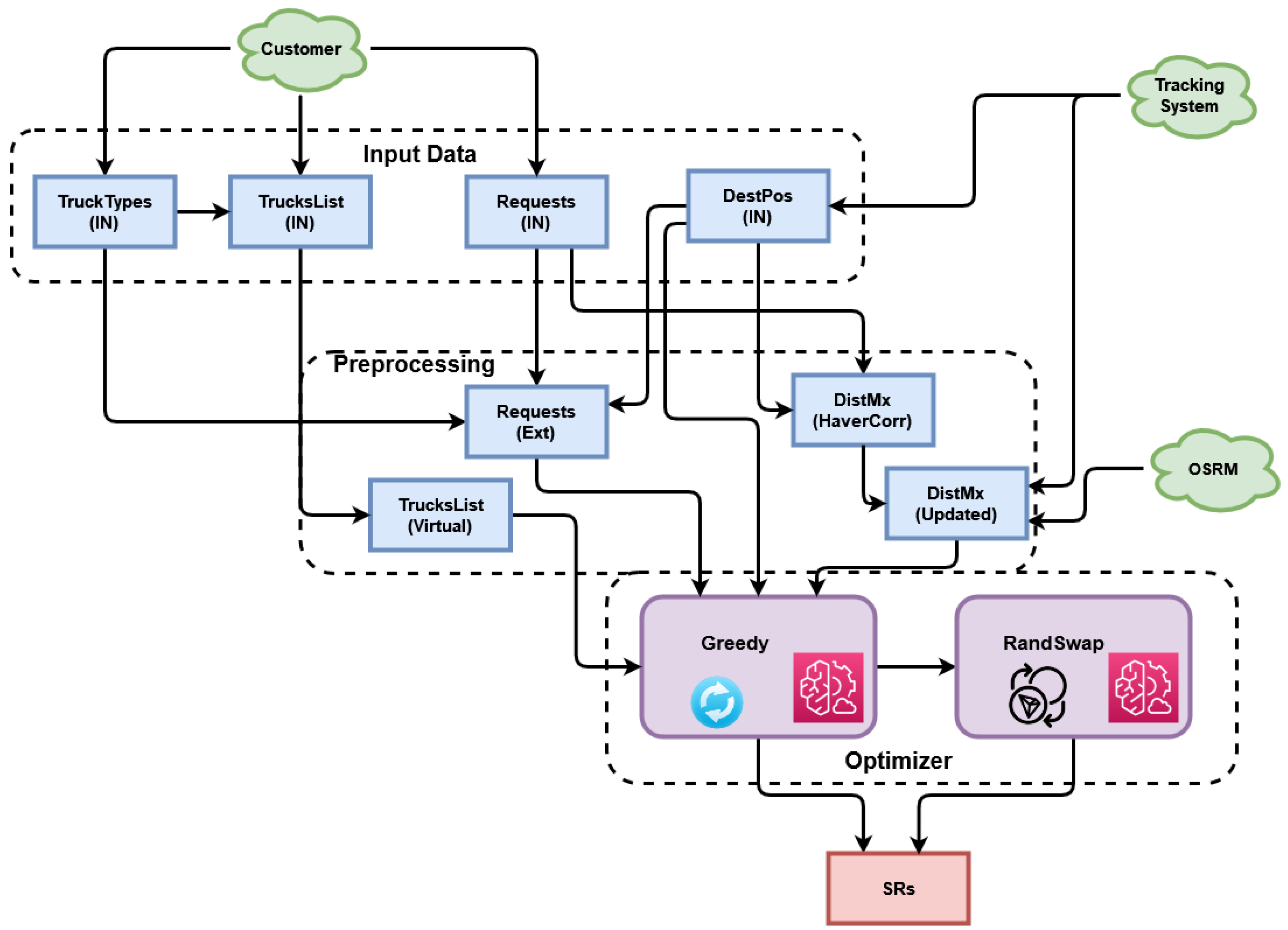
3. Materials and Methods

The prototype system, referring to the structure presented in Figure 1, was implemented using Python version 3.7 and the MySQL database. In the proposed considered scenario, the geolocalization data were obtained in integration with the GPS-based vehicle location system, the ABC-track system. The information was obtained thanks to the courtesy of the owners (ABC-Track Ltd. Company). Dedicated requests were sent to the address indicated in the Company documentation, using the HTTP—GET method. The getPoints service was used for receiving the information about individual points on the route map. The data was collected and processed using scripts written in Python programming language. The obtained data structures were imported to the newly created DataFrame object of the Pandas library in JSON format for further analysis in the optimization module. As a result of a query to the site, a list of objects was returned. Each of the objects is a representation of a particular point on the map and has the following information:

• pointId—unique identifier of the point.
• pointName—point name.
• pointLatitude—the latitude of the point.
• pointLongitude—the longitude of the point.

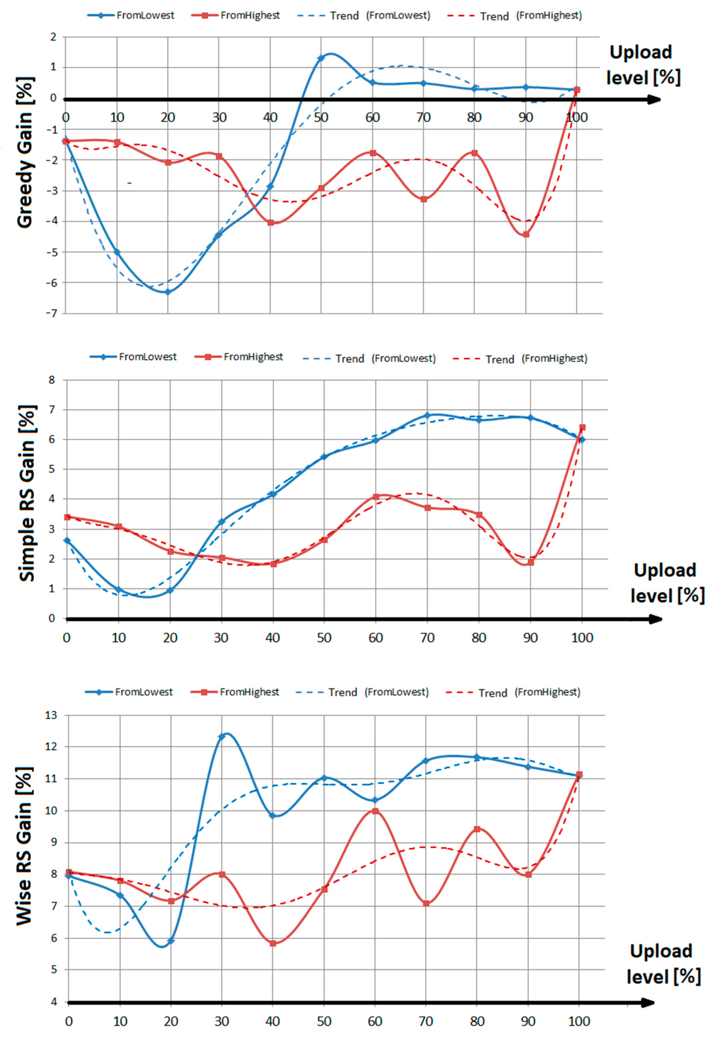
The distances between pairs of coordinates are obtained by the Table Service, offered in OSRM API. It calculates the length and duration of the fastest route between all pairs of given coordinates. All returned data were in JSON (JavaScript Object Notation) format, preprocessed using Python’s script, saved in a local database, and converted to tabular form (csv).

For the needs of the study, a two-stage optimization algorithm was developed and implemented in MathCad 13 software. It ensures a favorable balance between the degree of optimization and time consumption and is characterized by good scalability. The first and base stage is a version of the greedy algorithm, which guides the selection of orders for vehicles by the local best hop approach. It means a request is selected whose handling will have the most negligible possible impact on the growth of the cost function. In this case, total distance was the main optimization criterion. In the case of several equivalent candidates, the next criterion was the choice according to the largest truck-order heuristic principle. This stage is deterministic (i.e., it always returns the same result with the same input data set). In the second stage, the “greedy” solution is randomly adjusted based on the random swapping of orders assignments. It was a proprietary implementation of a variant of the 2-opt algorithm, often used to solve the traveling salesman problem [54]. Total fuel cost was the main optimization criterion in this stage. Three variants of the algorithm were used in the analyzes:

• Greedy only
• Greedy + Simple RandSwap and,
• Greedy + Wise RandSwap

Simple RandSwap relies on a random exchange of orders between two vehicles. If the swap generates a lower or equal cost—it is accepted, otherwise, it is rejected. In the Wise RandSwap algorithm, interchanges between vehicles with nearby routes are preferable.

The algorithm uses the following main inputs as shown in Figure 1: Requests, TrucksList, DestPos, and DistMx datasets. The DestPos and DistMx input data were imported from the mentioned csv file, returned by GIS/OSRM services, located in Kielce, Poland. Representative and actual input data of requests list and list of the vehicle was obtained from a local shipping company—Alma-Alpinex Join-Stock Company, which redistributes food products and manages a fleet of approx. 100 vehicles. The sample output problem solution (Service Records), including route sequences proposed by experienced planners, was obtained from the same source. Total 1103 pallets divided into 416 individual orders were redistributed to 202 destinations from one central depot. The six types of trucks with different capacities of 27, 21, 20, 18, 10, and 8 pallets were considered as candidates. The set of trucks was {20, 30, 20, 20, 20, 50}, this mean total 160 vehicles were taken into account.

4. Results

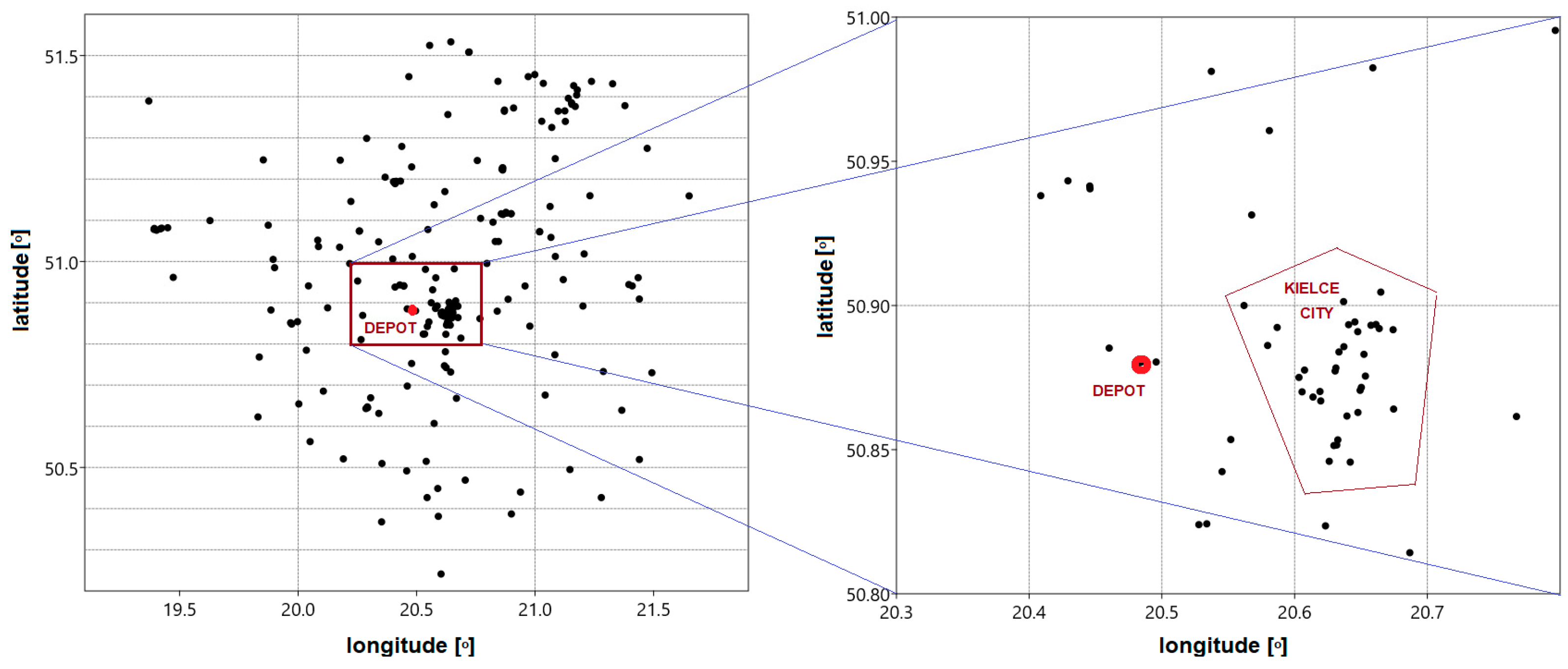
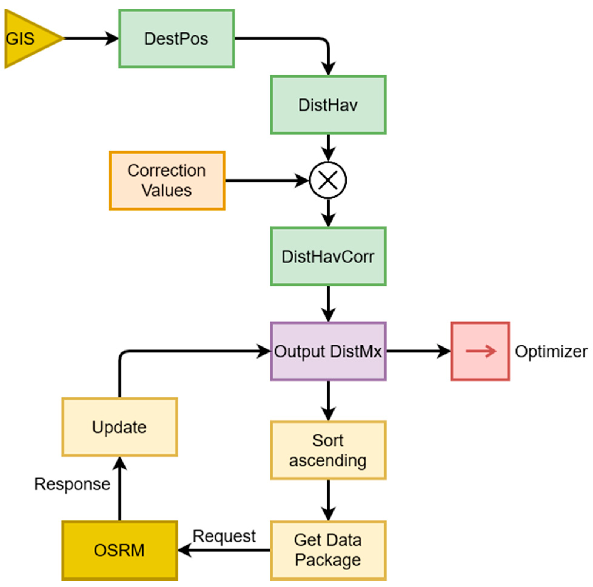
4.1. Getting the DestPos and DistMx

The basis for creating the DistMx matrix is a list of destinations (DestPos), containing at least the destination identifier (DestId) and geographical coordinates (latitude, longitude). Location coordinates are the basis for obtaining the distance value. A matrix with dimensions N × N will be created for N destinations, where N × (N-1) independent values exist. In the first step, an up-to-date list of destinations with their coordinates was obtained. Using the APIs the list includes all necessary 203 points (1 depot and 202 destinations) was downloaded. The presented destinations were located in an area estimated 160 (E-W) × 145 km (N-S). The spatial distribution of destinations is shown in Figure 2.

Next, to create a distance matrix, all destinations’ identifiers and geographical coordinates should be provided as starting and ending points. This service takes the following arguments: coords_src (list of geographical coordinates of the starting points), coords_dest (list of geographic coordinates of endpoints), ds_origin (list of identifiers of starting points) and ids_dest (list of endpoint identifiers). If a new destination appears, there is no need to recalculate the entire matrix. An additional script has been created, which works in such a way that it calculates the distances between a particular destination and the rest of the destinations. Thus, iterating over N destinations creates an N × N matrix. This way is to work around the limit on the engine side of the simultaneous number of data sent in the query. To add a new destination, it will only need to calculate one new column for a given destination, and transpose that column into a row, which then also add to the distance matrix. Such a solution is beneficial in the situation of a dynamically changing list of destinations. It has been experimentally found that updating the distance table in the event of an additional destination takes an average of a few seconds.

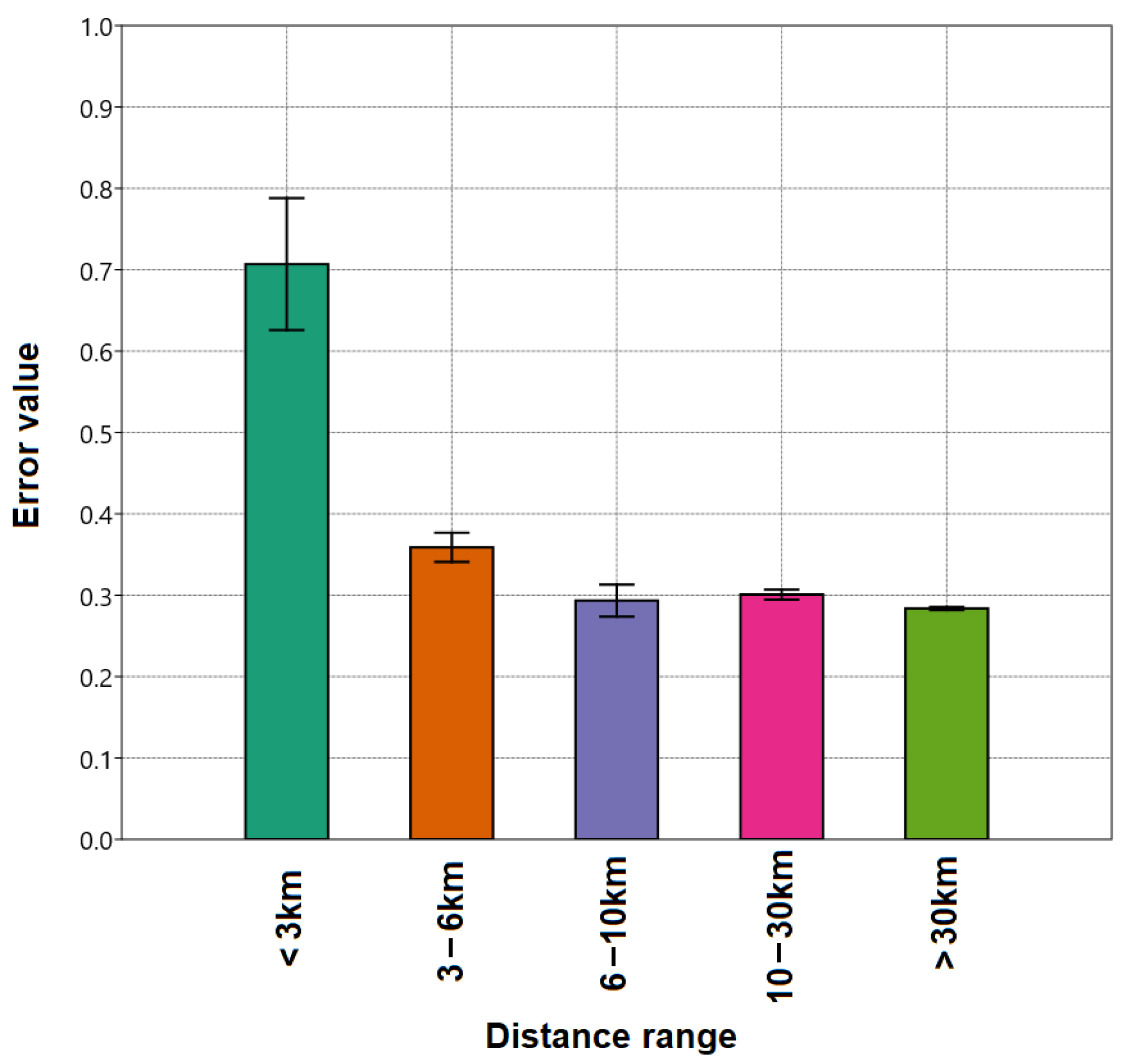
4.2. Temporary DistMx Calculation

The Authors observed that acquiring distance values from the OSRM website is possible, however, it may take a long time. In the case of sending individual inquiries, the time to complete the distance matrix was a few hours for N = 203 points. In the case of sending aggregated questions, it was possible to shorten this time to about tens of minutes. In unfavorable connectivity or problems with the service overflow, this time may be extended to unacceptable values (hours or more). Therefore, an alternative method of generating temporary values has been proposed. In the absence of current values obtained from the OSMR website, the distance can firstly be estimated based on the quasi-Euclidean metric. The following formula can be used to find the shortest distance (DistEucl) between two points located on a sphere with radius R.

$$DistEucl=2·R·arcsin\left(\sqrt{si{n}^2\left(\frac{\phi 1-\phi 2}{2}\right)+cos\left(\phi 1\right)·cos\left(\phi 2\right)·si{n}^2\left(\frac{\lambda 1-\lambda 2}{2}\right)}\right)$$

(1)

where

φ1, φ2 are the latitude of point 1 and 2, respectively; λ1, λ2 are the longitude of point 1 and 2, respectively; and R is the Earth’s radius (6371 km)

The distance determined from relation (1) is usually underestimated as the routes connecting two points are generally not a straight line. The relative underestimation error is derived from the simple Formula:

$$Err=\frac{DistOSRM-DistEucl}{DistEucl}$$

(2)

where

d_OSRM is the actual distance obtained from the OSRM service, and d_hav is the theoretical distance calculated from the dependence (1).

As both DistEucl and DistOSMR matrices are known, the dependence of the error value on the actual distance value was investigated. The analysis shows that for short distances (<3 km), the error value (underestimation level) may be significantly higher than for the entire sample. Therefore, the data set was segmented concerning the distance value, and for each segment, the average error value was determined with the 95% confidence interval (Figure 3). The preliminary analyzes show that for ultra-short distances (below 3 km), the theoretical value of the distance should be corrected (increased) by a factor as high as ~0.7. For longer distances (3–6 km), the correction factor can be estimated at the level of ~0.35, and for the remaining distances at the level of ~0.28.

Obtaining more correct values of the distance matrix can be achieved by designating an appropriate scaling function. This function can be an approximation of a DistOSRM = f(DistEucl) relation. On the other hand, it may be more advantageous to find a function that approximates the error value (2) dependence on the distance (1). In such a case, the general form of the function may be as follows:

$$Err\left(DistEucl\right)=a·e^{b·DistEucl}+c$$

(3)

In these considerations, the authors decided to approximate the error value using the Formula (3). The a, b, and c coefficients were determined by minimizing the mean square error (MSE). Optimization calculations were made using the non-linear generalized reduced gradient method [55], implemented in the Solver tool of Microsoft Excel software. For the data set the following coefficients were obtained: a = 0.766346, b = 1.25415 and c = 0.287121. Based on the dependence (3), the distribution of the correction coefficient as a function of the original value of the distance calculated from the dependence (1) was also determined.

As a result of applying the dependencies (1) and (3), a distance matrix named DistEuclCorr was calculated as follows.

$$DistEuclCorr\left[i,j\right]=\{\begin{array}{c}0 if DistEucl\left[i,j\right]=0\\ \left(Correction\left(DistEucl\left[i,j\right]\right)·DistEucl\left[i,j\right]\right) otherwise\end{array}$$

(4)

It was found that the arithmetic mean of the relative error between corresponding values of the DistOSRM and DistEuclCorr matrices was negligibly small (<0.00001). The standard deviation (SD) value has also been reduced to 0.1226 from the previous value of 0.1887. It was due to the introduction of the exponential component in the approximation function, as a result, the small values of the distance matrix were more effectively corrected. In contrast, the average value of non-zero elements of the DistEuclCorr matrix were about 0.5% higher than the corresponding value for DistOSRM.

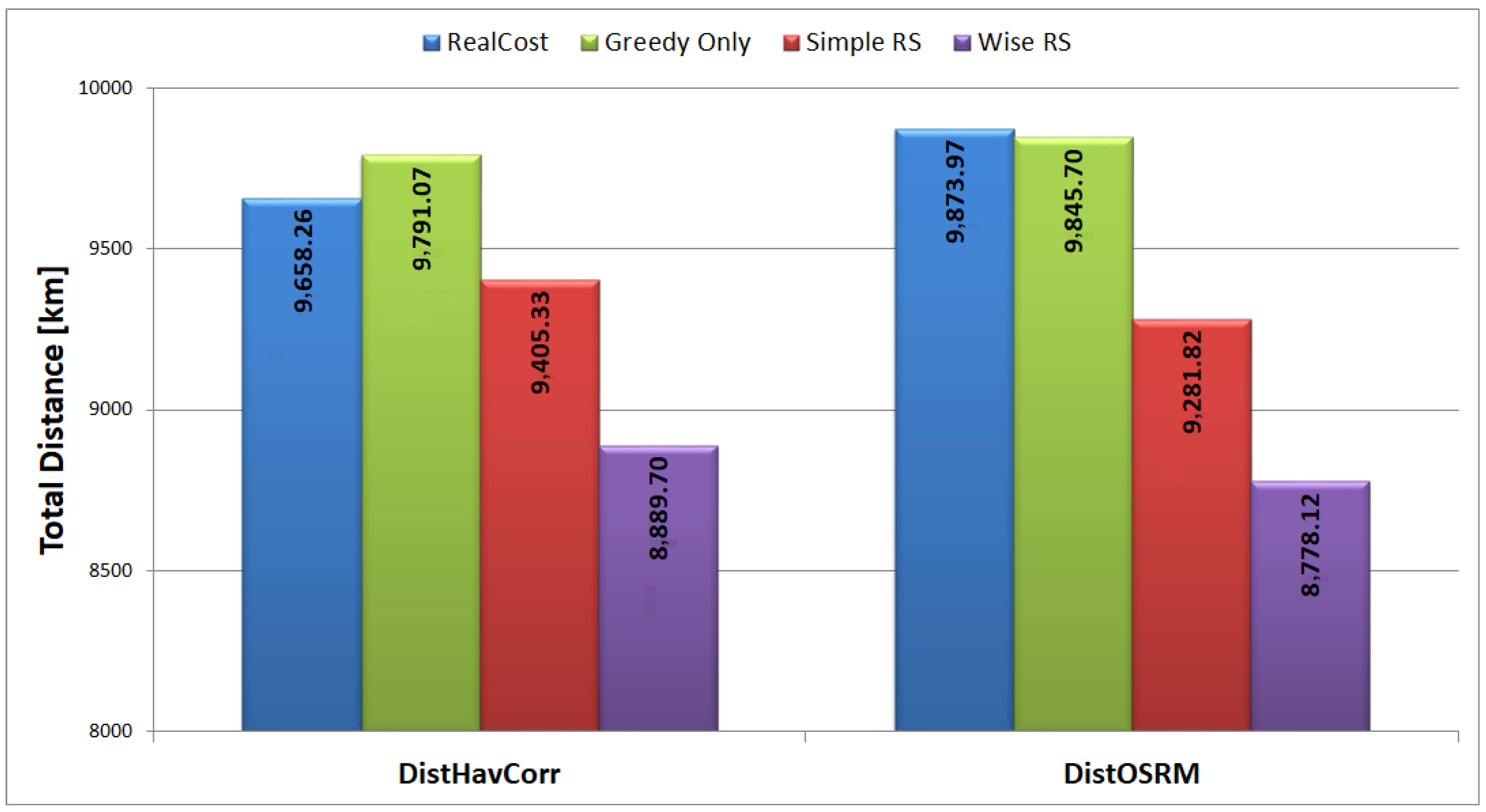
4.3. Infuence of Distance Matrix Upload on Optimizer Cost Reduction

One of the best methods of estimating the effectiveness of an optimizer is to compare the returned solutions with the solutions proposed by experienced planners. As mentioned in Section 3, both the order parameters (the size of requests, types and load capacity of vehicles, the location of destinations) and the proposed “manual” solution, including route sequences, were known. Thanks to this, it was possible to calculate the actual distance (RealDist) as the resulting cost function. This value was a reference to the values obtained in the optimizer (OutCost). Both the RealDist and OutCost values depend on the form of the assumed distance matrix. The open question is how the optimizer cost reduction (Gain) depends on the state of the matrix used. This parameter can be defined by Formula (5).

$$Gain [\%]=\frac{RealDist-OutCost}{RealDist}\times 100$$

(5)

Using the optimization algorithms described in Section 3, OutCost values were obtained for all free algorithm variants: Greedy, Simple RandSwap, and Wise RandSwap. In the RandSwap stage, the five attempts with 100,000 iterations were calculated due to its stochastic feature, and arithmetic mean value was reported. The best variant, as expected, was the Wise Rand Swap algorithm.

Figure 4 compares the cost values (route distance) obtained for the two proposed forms of the used distance matrix. Although the average distance values in DistEuclCorr were slightly higher than DistOSMR (~0.5%), the actual distance (cost) calculated based on the result sequences was higher (by ~2.2%) for the case of using the temporary matrix. This result may be due to the fact that the proposed routes do not contain the hops corresponding to the most significant values in the distance matrix.

For the temporary distance matrix (DistEuclCorr), greedy optimization results in negative efficiency. It is then improved in the RandSwap stage. However, in the case of using actual distances obtained from the OSRM (DistOSRM) service, the “greedy” stage is characterized by positive cost reduction. The observation shows how important the actuality of the distance matrix is from the point of view of the optimizer’s effectiveness. Assuming the theoretical values based on haversine metrics, one can erroneously hypothesize that the greedy algorithm is not sufficiently effective (Gain = −1.37%) in the process of planning deliveries. Meanwhile, substituting actual values contradicts previous observations.

The order of updating individual elements of the distance matrix is another aspect worth analyzing. As mentioned, it may take several hours to get all the actual distance values. Communication interruptions and service loads must be taken into account. For this reason, it is advisable to update the DistEuclCorr matrix values successively. The analysis of the resulting sequence of the optimization algorithm allowed us to make the following observations. First, the maximum value of a single distance (hop) is comparable to half of the maximum value in the distance matrix. It means that larger values do not need to be updated urgently. It was estimated that such values constitute ~10% of all matrix elements. Moreover, approx. 60% of the appeals used in the case of distances shorter than 20 km. For this reason, it makes sense to update the short distances first. They are, firstly, more often used in the optimizer, and secondly, the relative error value is more significant for smaller distance values.

According to the assumptions, more in-depth analyses were carried out by examining the impact of the update level (in %) on cost reduction. A total of 20 different partially-updated “mixed-matrices” were generated, divided into two series. In the first series, matrices data was uploaded starting from the lowest distance values and the second starting from the highest ones, respectively. It started from 0% (DistEuclCorr) and increased by 10% up to 100% (DistOSRM). The values of the Gain coefficient were calculated for any cases.

Table 1. Cost reduction for different distance matrix types.

Algorithms:	DistEuclCorr	Mixed-Matrix (50% from Lowest)	Mixed-Matrix (50% from Highest)	DistOSRM
Greedy Only	−1.38%	1.31%	−2.90%	0.29%
Simple RS	2.62%	5.43%	2.64%	6.00%
Wise RS	7.96%	11.03%	7.54%	11.10%

, presents the calculated values of the cost reduction (Gain) for selected distance matrices

Particularly in the case of the Wise RS algorithm, it is noted that the mixed-matrix containing the 50% update of the smallest coefficients exhibits similar properties to the DistOSRM target matrix. In contrast, the mixed-matrix containing 50% of the highest index updates has the characteristics of the DistEuclCorr temporary matrix. More detailed results are represented in Figure 5, where an evolution of the calculated Gain value is presented.

For all cases, the cross-section (represented by the trend lines—fit of 6-order polynomial) takes the form of a characteristic hysteresis. The trend-line for the series “from lowest” seems to be clearly more favorable from the point of view of stabilizing the expected value of the Gain coefficient. In fact, with about 40–50% of updates, the Mixed Matrix exhibits the characteristics of the target matrix. On the other hand, updating the matrix in the “from highest” variant seems to be the wrong approach. It turns out that even with an 80–90% update level, the expected results are significantly different from the final one.

5. Discussion

The correct form of the distance matrix is a crucial parameter influencing the effectiveness of the optimization algorithm used in the optimizer. Many previous papers discussed the possibility of obtaining distance matrices from the corrected Euclidean distance. To approximate the actual distance, Cooper [56] proposed using a factor of the curvature of the road, which can be calculated as the ratio between the actual distance and the Euclidean distance [57]. For UK roads, a value of 1.2 was proposed by Barthélemy [58] for the correction factor, which has subsequently been widely accepted and used in the scientific community. According to [59], correction factors of 1.25 for the long haul and 1.30 for an urban drayage area are used. The listed values are slightly lower than those proposed in this article. Based on the approximations made, the correction coefficient can be assumed at the level of 1.287 for distances above 10 km, which is a value comparable to the proposals appearing in the cited papers. Note that in the case of the space represented by the Manhattan metric, the value of the correction factor should not exceed √2 ≈ 1.414. In reality, however, a more significant correction should be made, especially for very short distances below 3 km. As shown in Figure 3 the correction factor can be as high as 1.7 for ultra-short distances.

The discrepancies between values proposed in this work and values proposed in mentioned above papers suggest that receiving more real data obtained from Mapping API services is highly recommended. Moreover, the presented results indicate that the evaluation of the algorithm’s effectiveness may be determined by the smallest distance values (the lowest weights of the graph representing the transport problem). As shown in Figure 5 (trend “from highest”), the last 10% of the lowest coefficients significantly affect the calculated Gain value. It makes sense as a more significant relative error characterizes these values. On the other hand, the absolute error may be more significant for longer distances. It shows the advantage of the reverse approach, where the update should start with the highest values and was confirmed by analyzing the correlations between mixed-matrix and DistOSRM.

The observed trend of the Gain coefficient should be linked by a change in the rank of individual elements of the distance matrix. The behavior of two correlation coefficients (Pearson’s linear and Spearman’s rank) was analyzed. The appropriate values were calculated between the final DistOSRM matrix and successively updated mix-matrices for both the “from lowest” and “from highest” variants. Figure 6 shows all four corresponding graphs. In the case of Pearson’s correlation, significant differences in the formation of the correlation are observed during the update of the distance matrix between the “from lowest” and “from highest” approach. Moreover, the chart suggests that during the update of the values from the highest, the correlation sooner tends to 1, which negates the earlier thesis. However, a more reliable parameter is the rank correlation coefficient. In this case, the changes in the trend are similar. In fact, the correlation analysis does not provide backgrounds for selecting the “from lowest” variant.

However, the choice of the “from lowest” approach can be defended by looking at the histogram representing the distribution of the cost values of single jumps proposed by the optimization algorithm. A histogram represents a distribution of single-hop OSRM distances reported in optimizer solution was calculated (Figure 7A).

As shown in the proposed solutions, shorter distances, below 30 km, are reused more often. It indicates that it is the shorter distances that should be updated first. On the other hand, the share of short distances in the total cost is lower. After scaling the count value by the distance value, a different distribution is obtained (Figure 7B). For example, hops with a cost value of 85–95 km, corresponding to the return routes, have the highest contribution to the total cost. It may indicate consideration of a mixed approach in the future, such as from peripheral to center. However, in its present state, it suggests the superiority of the “from lowest” approach.

According to the obtained results, the following scheme was proposed (Figure 8).

First, from the GIS outside system, the actual DestPos list is downloaded. Next, the distance matrix based on the quasi-euclidean distance (1) is calculated and corrected according to Formula (4). The resulting data are the initial (temporary) set used by the optimization algorithm. Simultaneously, an additional list containing distances is sorted in increasing order and segmented into data packages, preferably no more than 200 values per one package. Next, the special agent is responsible for sending inquiries updating the distance values to the OSRM service, starting from the smallest matters. After receiving a positive answer, the process of successive DistMx update takes place.

6. Conclusions

In the article, some aspects of the optimization issues in WFM and VRP problem were discussed. The prototype system that supports the routing optimization process of VRP issues in real-time was proposed. This system is designed to quickly and efficiently allocate individual requests to transport resources. It also considers frequent changes in the location of the destination and transport costs. In the case of dynamically changing destination lists, constant updating of the matrix form is required. The update process is possible thanks to services such as Mapping APIs such as OSRM service, but it can take a long time. The article proposes a method of initial initialization of the matrix form and then a reasonable approach to successive updating of individual values. It also means that integrating GIS systems, GPS systems, and optimization algorithms is a beneficial solution. It was also shown that the proper and fast upgrading of the distance matrix may affect the assessment of the optimization effectiveness. Obsolete or approximate d [i, j] values may significantly affect the evaluation of the effectiveness of a certain class of algorithms, in particular the greedy algorithm. Differences of more than 7% were found here. It has been noticed that it is more advantageous to start the refreshing process from the smallest values in arduous requesting updated data. The proposed approach is not due to the fact that the relative error is more significant for small distances, but that the optimization algorithm often refers to the lowest values.

As mentioned, the experiments and analyses performed are part of a more comprehensive project. They aim to develop a practical, fast, and effective quasi-optimal resource allocation algorithm in the dynamically changing conditions of the request space. Such issues were named ‘Agile Workforce Management’ and constitute an advantage over the classic static solutions.

References

1. Dantzig, G.; Ramser, J. The truck dispatching problem. Manag. Sci. 1959, 6, 80–91. [Google Scholar] [CrossRef]
2. Clarke, G.; Wright, J.W. Scheduling of vehicles from central depot to a number of delivery points. Oper. Res. 1964, 12, 568–582. [Google Scholar] [CrossRef]
3. Hota, J.; Ghosh, D. Workforce Analytics Approach: An Emerging Trend of Workforce Management. AIMS Int. J. Manag. 2013, 7, 167–179. Available online: https://ssrn.com/abstract=2332713 (accessed on 5 September 2021).
4. Workforce Management: How to Optimize Team Productivity. Available online: https://asana.com/pl/resources/workforce-management (accessed on 5 September 2021).
5. Konstantakopoulos, G.D.; Gayialis, S.P.; Kechagias, E.P. Vehicle routing problem and related algorithms for logistics distribution: A literature review and classification. Oper. Res. Int. J. 2020, 1–30. [Google Scholar] [CrossRef]
6. Zhang, H.; Ge, H.; Yang, J.; Tong, Y. Review of Vehicle Routing Problems: Models, Classification and Solving Algorithms. Arch. Comput. Method Eng. 2021, 1–27. [Google Scholar] [CrossRef]
7. Psaraftis, H.S.; Wen, M.; Kontovas, C.A. Dynamic vehicle routing problems: Three decades and counting. Networks 2016, 67, 3–31. [Google Scholar] [CrossRef] [Green Version]
8. Braekers, K.; Ramaekers, K.; Van Nieuwenhuyse, I. The vehicle routing problem: State of the art classification and review. Comput. Ind. Eng. 2016, 99, 300–313. [Google Scholar] [CrossRef]
9. Katoch, S.; Chauhan, S.S.; Kumar, V. A review on genetic algorithm: Past, present, and future. Multimed. Tools Appl. 2021, 80, 8091–8126. [Google Scholar] [CrossRef]
10. Guilmeau, T.; Chouzenoux, E.; Elvira, V. Simulated annealing: A review and a new scheme. In Proceedings of the SSP 2021—IEEE Statistical Signal Processing Workshop, Rio de Janeiro, Brazil, 11–14 July 2021; pp. 1–5. Available online: https://hal.inria.fr/hal-03275401 (accessed on 12 November 2021).
11. Suman, B.; Kumar, P. A Survey of Simulated Annealing as a Tool for Single and Multiobjective Optimization. J. Operl. Res. Soc. 2006, 57, 1143–1160. Available online: http://www.jstor.org/stable/4102365 (accessed on 12 November 2021). [CrossRef]
12. Coronado de Koster, O.A.; Domínguez-Navarro, J.A. Multi-Objective Tabu Search for the Location and Sizing of Multiple Types of FACTS and DG in Electrical Networks. Energies 2020, 13, 2722. [Google Scholar] [CrossRef]
13. Chen, J.; Gui, P.; Ding, T.; Na, S.; Zhou, Y. Optimization of Transportation Routing Problem for Fresh Food by Improved Ant Colony Algorithm Based on Tabu Search. Sustainability 2019, 11, 6584. [Google Scholar] [CrossRef] [Green Version]
14. Cordon, O.; Herrera, F.; Stützle, T. A review on the ant colony optimization metaheuristic: Basis, models and new trends. Mathw. Soft Comput. 2003, 9, 141–175. [Google Scholar]
15. Jain, N.K.; Nangia, U.; Jain, J. A Review of Particle Swarm Optimization. J. Inst. Eng. India Ser. 2018, 99, 407–411. [Google Scholar] [CrossRef]
16. Lopes Silva, M.A.; de Souza, S.R.; Freitas Souza, M.J.; de França Filho, M.F. Hybrid metaheuristics and multi-agent systems for solving optimization problems: A review of frameworks and a comparative analysis. Appl. Soft Comput. 2018, 71, 433–459. [Google Scholar] [CrossRef]
17. Talbi, E.G. Hybrid Metaheuristics for Multi-Objective Optimization. J. Algorithms Comput. Technol. 2015, 9, 41–63. [Google Scholar] [CrossRef] [Green Version]
18. Boelaert, M.; Arbyn, M.; Van der Stuyft, P. Geographical information systems (GIS), gimmick or tool for health district management. Trop. Med. Int. Health 1998, 3, 163–165. [Google Scholar] [CrossRef]
19. Gatrell, A.C.; Elliot, S.J. Geographies of Health: An Introduction, 2nd ed.; Wiley-Blackwell: Malden, MA, USA, 2009. [Google Scholar]
20. Shen, L.; Stopher, P.R. Review of GPS Travel Survey and GPS, Data-Processing Methods. Transp. Rev. 2014, 34, 316–334. [Google Scholar] [CrossRef]
21. Tsakiri, M.; Stewart, M.; Forward, T.; Sandison, D.; Walker, J. Urban Fleet Monitoring with GPS and GLONASS. J. Navig. 1998, 51, 382–393. [Google Scholar] [CrossRef]
22. Hu, Y.; Chiu, Y.; Hsu, C.; Chang, Y. Identifying Key Factors for Introducing GPS-Based Fleet Management Systems to the Logistics Industry. Math. Probl. Eng. 2015, 2015, 413203. [Google Scholar] [CrossRef] [Green Version]
23. Pluvinet, P.; Gonzalez-Feliu, J.; Ambrosini, C. GPS data analysis for understanding urban goods movement. Procedia Soc. Behav. Sci. 2012, 39, 450–462. [Google Scholar] [CrossRef] [Green Version]
24. Rojas, B.; Bolaños, C.; Salazar-Cabrera, R.; Ramírez-González, G.; Pachón de la Cruz, A.; Madrid Molina, J.M. Fleet Management and Control System for Medium-Sized Cities Based in Intelligent Transportation Systems: From Review to Proposal in a City. Electronics 2020, 9, 1383. [Google Scholar] [CrossRef]
25. Zambrano-Martinez, J.L.; Calafate, C.T.; Soler, D.; Lemus-Zúñiga, L.G.; Cano, J.C.; Manzoni, P.; Gayraud, T. A centralized route-management solution for autonomous vehicles in urban areas. Electronics 2019, 8, 722. [Google Scholar] [CrossRef] [Green Version]
26. Weyns, D.; Holvoet, T.; Helleboogh, A. Anticipatory vehicle routing using delegate multi-agent systems. In Proceedings of the 2007 IEEE Intelligent Transportation Systems Conference, Seattle, WA, USA, 30 September–3 October 2007; pp. 87–93. [Google Scholar]
27. Adewara, K.A. An Evaluation of Open Source Geographic Information Systems Routing Tools in Vaccine Delivery in Kano State, Northern Nigeria. In Proceedings of the Free and Open Source Software for Geospatial (FOSS4G) Conference, Seoul, Korea, 14–19 September 2015; Volume 15. [Google Scholar] [CrossRef]
28. Lovelace, R. Open source tools for geographic analysis in transport planning. J. Geogr. Syst. 2021, 23, 547–578. [Google Scholar] [CrossRef]
29. Rauf, I.; Troubitsyna, E.; Porres, I. A systematic mapping study of API usability evaluation methods. Comp. Sci. Rev. 2019, 33, 49–68. [Google Scholar] [CrossRef]
30. Jambu, M. Exploratory and Multivariate Data Analysis; Academic Press: Paris, France, 1991. [Google Scholar]
31. Archetti, C.; Speranza, M.G. The Split Delivery Vehicle Routing Problem: A Survey. In The Vehicle Routing Problem: Latest Advances and New Challenges; Operations Research/Computer Science Interfaces 43; Golden, B., Raghavan, S., Wasil, E., Eds.; Springer: Boston, MA, USA, 2008. [Google Scholar]
32. Zhang, Q.; Wei, L.R.; Hu, R.; Yan, R.; Li, L.H.; Zhu, X.N. A Review on the Bin Packing Capacitated Vehicle Routing Problem. Adv. Mater. Res. 2013, 853, 668–673. [Google Scholar] [CrossRef]
33. Kritikos, M.N.; Ioannou, G. The heterogeneous fleet vehicle routing problem with overloads and time windows. Int. J. Prod. Econ. 2013, 144, 68–75. [Google Scholar] [CrossRef]
34. Sitek, P.; Wikarek, J. Capacitated vehicle routing problem with pick-up and alternative delivery (CVRPPAD): Model and implementation using hybrid approach. Ann. Oper. Res. 2019, 273, 257–277. [Google Scholar] [CrossRef] [Green Version]
35. Dijkstra, E.W. A note on two problems in connexion with graphs. Numer. Math. 1959, 1, 269–271. [Google Scholar] [CrossRef] [Green Version]
36. Bruniecki, K.; Chybicki, A.; Moszyński, M.; Bonecki, M. Towards solving heterogeneous fleet vehicle routing problem with time windows and additional constraints: Real use case study. In Proceedings of the 2016 Federated Conference on Computer Science and Information Systems (FedCSIS), Gdansk, Poland, 11–14 September 2016. [Google Scholar]
37. Panicker, V.V.; Mohammed, I.O. Solving a Heterogeneous Fleet Vehicle Routing Model—A practical approach. In Proceedings of the IEEE International Conference on System, Computation, Automation and Networking (ISCAN), Pondicherry, India, 6–7 July 2018; pp. 1–5. [Google Scholar] [CrossRef]
38. Zhang, J.; Yu, M.; Feng, Q.; Leng, L.; Zhao, Y. Data-Driven Robust Optimization for Solving the Heterogeneous Vehicle Routing Problem with Customer Demand Uncertainty. Complexity 2021, 2021, 6634132. [Google Scholar] [CrossRef]
39. Ioannou, G.; Kritikos, M.; Prastacos, G. A Greedy Look-Ahead Heuristic for the Vehicle Routing Problem with Time Windows. J. Oper. Res. Soc. 2001, 52, 523–537. [Google Scholar] [CrossRef]
40. Dondo, R.; Cerda, J. A cluster-based optimization approach for the multi-depot heterogeneous fleet vehicle routing problem with time windows. Eur. J. Oper. Res. 2007, 176, 1478–1507. [Google Scholar] [CrossRef]
41. Mehrjerdi, Y.Z.; Nadizadeh, A. Using greedy clustering method to solve capacitated location-routing problem with fuzzy demands. Eur. J. Oper. Res. 2013, 229, 75–84. [Google Scholar] [CrossRef]
42. Karner, T.; Weninger, B.; Schuster, B.; Fleck, S.; Kaminger, I. Improving Road Freight Transport Statistics by Using a Distance Matrix. Aust. J. Stat. 2017, 46, 65–80. [Google Scholar] [CrossRef]
43. Zgonc, B.; Tekavčič, M.; Jakšič, M. The impact of distance on mode choice in freight transport. Eur. Trans. Res. Rev. 2019, 11, 10. [Google Scholar] [CrossRef]
44. Kuehnel, N.; Ziemke, D.; Moeckel, R.; Nagel, K. The end of travel time matrices: Individual travel times in integrated land use/transport models. J. Trans. Geogr. 2020, 88, 1–12. [Google Scholar] [CrossRef]
45. Henzinger, M.; Paz, A.; Schmid, S. On the Complexity of Weight-Dynamic Network Algorithms. In Proceedings of the IFIP Networking Conference, Espoo and Helsinki, Finland, 21–24 June 2021; pp. 1–9. [Google Scholar] [CrossRef]
46. Gutenberg, M.P.; Wulff-Nilsen, C. Fully-Dynamic All-Pairs Shortest Paths: Improved Worst-Case Time and Space Bounds. arXiv 2020, arXiv:2001.10801. [Google Scholar]
47. The Distance Matrix API for Transport Logistics and Freight. Available online: https://distancematrix.ai/logistics-solutions (accessed on 5 September 2021).
48. TravelTime Distance Matrix API. Available online: https://traveltime.com/features/distance-matrix (accessed on 5 September 2021).
49. Time-Distance Matrix and Three Ways to Use It. Available online: https://www.geoapify.com/time-distance-matrix-and-three-ways-to-use-it (accessed on 5 September 2021).
50. Google Maps Platform. Available online: https://developers.google.com/maps/documentation/distance-matrix/overview (accessed on 5 September 2021).
51. Open Routing Source Machine—Modern C++ Routing Engine for Shortest Paths in Road Networks. Available online: http://project-osrm.org/ (accessed on 5 September 2021).
52. Akanbi, A.K.; Agunbiade, O.Y. Integration of a city GIS data with Google Map API and Google Earth API for a web based 3D Geospatial Application. arXiv 2013, arXiv:1312.0130. [Google Scholar]
53. Favretto, A. API, Cloud computing, WebGIS and cartography. Netcom 2010, 24-3/4, 245–260. [Google Scholar] [CrossRef]
54. Karagul, K.; Aydemir, E.; Tokat, S. Using 2-Opt based evolution strategy for travelling salesman problem. Int. J. Optim. Control Theor. Appl. 2016, 6, 103–113. [Google Scholar] [CrossRef] [Green Version]
55. Facó, J.L.D. A Generalized Reduced Gradient Algorithm for Solving Large-Scale Discrete-Time Nonlinear Optimal Control Problems. IFAC Proc. Vol. 1989, 22, 45–50. [Google Scholar] [CrossRef]
56. Cooper, J.C. The use of straight line distances in solutions to the vehicle scheduling problem. J. Oper. Res. Soc. 1983, 34, 419. [Google Scholar] [CrossRef]
57. Kim, N.S.; Van Wee, B. The relative importance of factors that influence the break-even distance of intermodal freight transport systems. J. Transp. Geogr. 2011, 19, 859–875. [Google Scholar] [CrossRef]
58. Barthélemy, M. Spatial networks. Phys. Rep. 2011, 499, 1–101. [Google Scholar] [CrossRef] [Green Version]
59. Domínguez-Caamaño, P.; Benavides, J.A.C.; Prado, J.C.P. An improved methodology to determine the wiggle factor: An application for Spanish road transport. Braz. J. Oper. Prod. Manag. 2016, 1, 52. [Google Scholar] [CrossRef] [Green Version]
Figure 1. Optimization system including upgrading of geopositioning data.
Applsci 11 10933 g001
Figure 2. Location of destinations in geographical coordinates.
Applsci 11 10933 g002
Figure 3. Bar plot with errors representing relative error values in the different distance range.
Applsci 11 10933 g003
Figure 4. Optimizer effectivity vs. type of distance matrix.
Applsci 11 10933 g004
Figure 5. Evolution of cost reduction in case dynamic matrix upload (starting from highest and lowest matrix values, respectively).
Applsci 11 10933 g005
Figure 6. Pearson’s and Spearman’s correlation coefficient between DistOSRM matrix values and successively updated mixed-matrix.
Applsci 11 10933 g006
Figure 7. Distribution of single hop distances reported in optimizer solution (A) and cost contribution vs. distance value (B).
Applsci 11 10933 g007
Figure 8. “Smart” geopositioning updating of the distance matrix.
Applsci 11 10933 g008