Integration of ERT, IP and SP Methods in Hard Rock Engineering

Abstract

Investigation of a hard rock site for the development of engineered structures mainly depends on the delineation of weathered and unweathered rock, and the fractures/faults. Traditionally, borehole tests are used in such investigations. However, such approaches are expensive and time-consuming, require more equipment, cannot be conducted in steep topographic areas, and provide low coverage of the area with point measurements only. Conversely, geophysical methods are non-invasive, economical, and provide large coverage of an area through both vertical and lateral imaging of the subsurface. The geophysical method, electrical resistivity tomography (ERT), can reduce a significant number of expensive drilling tests in geotechnical investigations. However, a geophysical method alone may provide ambiguity in the interpretation of the subsurface, such as electrical resistivity cannot differentiate between water and clay content. Such uncertainty can be improved by the integration of ERT with induced polarization (IP). Similarly, self-potential (SP) can be integrated with other geophysical methods to delineate the groundwater flow. In this contribution, we integrated three geophysical methods (ERT, IP and SP) to delineate the weathered and unweathered rock including the weathered/unweathered transition zone, to detect the fractures/faults, and to map the groundwater flow. Based on ERT, IP and SP results, we develop a geophysical conceptual site model which can be used by site engineers to interpret/implement the findings for build-out. Our approach fills the gaps between the well data and geological model and suggests the most suitable places for the development of engineered structures in the hard rock terrains.

1. Introduction

Given natural heterogeneity, the evaluation of hard rock sites for the construction of engineered structures is a challenging task for planners and engineers. The sustainable design of structures depends on the accurate evaluation of the subsurface geological model [1]. The uncertainty in the subsurface interpretation may cause structure failure [2,3]. A geotechnical site investigation requires time, expenses, and evaluation of subsurface heterogeneity. There is a need to use techniques so that planners can overcome the challenges of a costly and longtime commitment [4]. The construction sites without any proper geotechnical investigation result in building collapse in many developing countries [5]. In the hard rock terrains, the subsurface geological knowledge about the weathered and unweathered rock and the fractures/faults needs to be known for the success of the engineering construction [6]. The weathered zones and fractures/faults are mainly created by tectonic, chemical, erosion and weathering processes. The weathered/fractured zones are mainly associated with groundwater occurrence in the hard rock [7,8]. Therefore, identification of the weathered/fractured zones saturated with groundwater is essential to avoid locating engineered structures within potential failure zones [3,6].

Traditionally, boreholes are carried out to acquire subsurface geological knowledge [9,10]. However, given safety and accessibility issues, it is a challenging task to conduct such tests in steep topographic areas [11,12]. In addition, the drilling approaches are expensive, time-consuming, need heavy equipment, offer low coverage of point measurements only, and cannot provide lateral information on the subsurface [13,14]. Thus, the conventional tests cause uncertainties in the geological model which may lead planners to locate engineered structures at locations where failure is more likely [15]. Therefore, an alternative approach of traditional geotechnical techniques is necessary, which can delineate the subsurface between borehole locations prior to the engineering construction and thus bring a sigh of relief to the engineers.

In the past years, many researchers have used geophysical methods in their investigations [16,17,18,19,20,21,22,23,24,25,26,27,28]. Geophysical methods, such as electrical resistivity tomography (ERT), induced polarization (IP) and self-potential (SP) are non-invasive, fast, economical, user friendly, and provide lateral and vertical mapping of the subsurface for large coverage areas [22,29]. ERT is widely used in environmental and geotechnical investigations [3,17,20,23]. ERT measures electrical resistivity which has a wide range of values and varies with rock type. Unweathered rock has high resistivity, while weathered rock has lower values [10]. Thus, ERT can be used to map the weathered and unweathered zones. However, ERT alone cannot distinguish between water and clay content, since low resistivity suggests water, as well as clay content in the saturated zone [3]. The clay content causes instability in the foundation rock of the engineering structures. Recently, the integration between two or more geophysical methods has been very successful to reduce the uncertainty caused by a single geophysical method [9,24,25]. Integration between IP and ERT can remove the uncertainty caused by low values of electrical resistivity as high IP values indicate clay content whereas low IP values reveal water content [30,31]. In addition, ERT coupled with IP can detect the saturated weathered/fractured zones more efficiently since low values of electrical resistivity and chargeability suggest water content [3]. The negative values of SP suggest groundwater flow; thus, SP is very effective to evaluate the groundwater flow mainly along the weathered/fractured zones [10,32].

In this work, we performed an integrated geophysical survey of ERT, IP and SP at a highly heterogeneous hard-rock terrain in order to evaluate the subsurface for site suitability prior to engineering construction. The electrical resistivity obtained by ERT was used to delineate the distinct subsurface layers, such as the topsoil layer, weathered layer, weathered/unweathered transition zone and the unweathered rock at the bottom. Zones of higher clay content were delineated with the integration between ERT and IP. The groundwater flow path was inferred by SP. The 2D models of integrated geophysical methods provide a thorough insight into the subsurface. Compared with conventional geotechnical studies, our contribution reduces the uncertainty caused by the spatially limited data, provides a more accurate geological model via lateral and vertical (2D) imaging of the large area, and suggests the most suitable places for the development of engineering structures in highly heterogeneous hard-rock terrain.

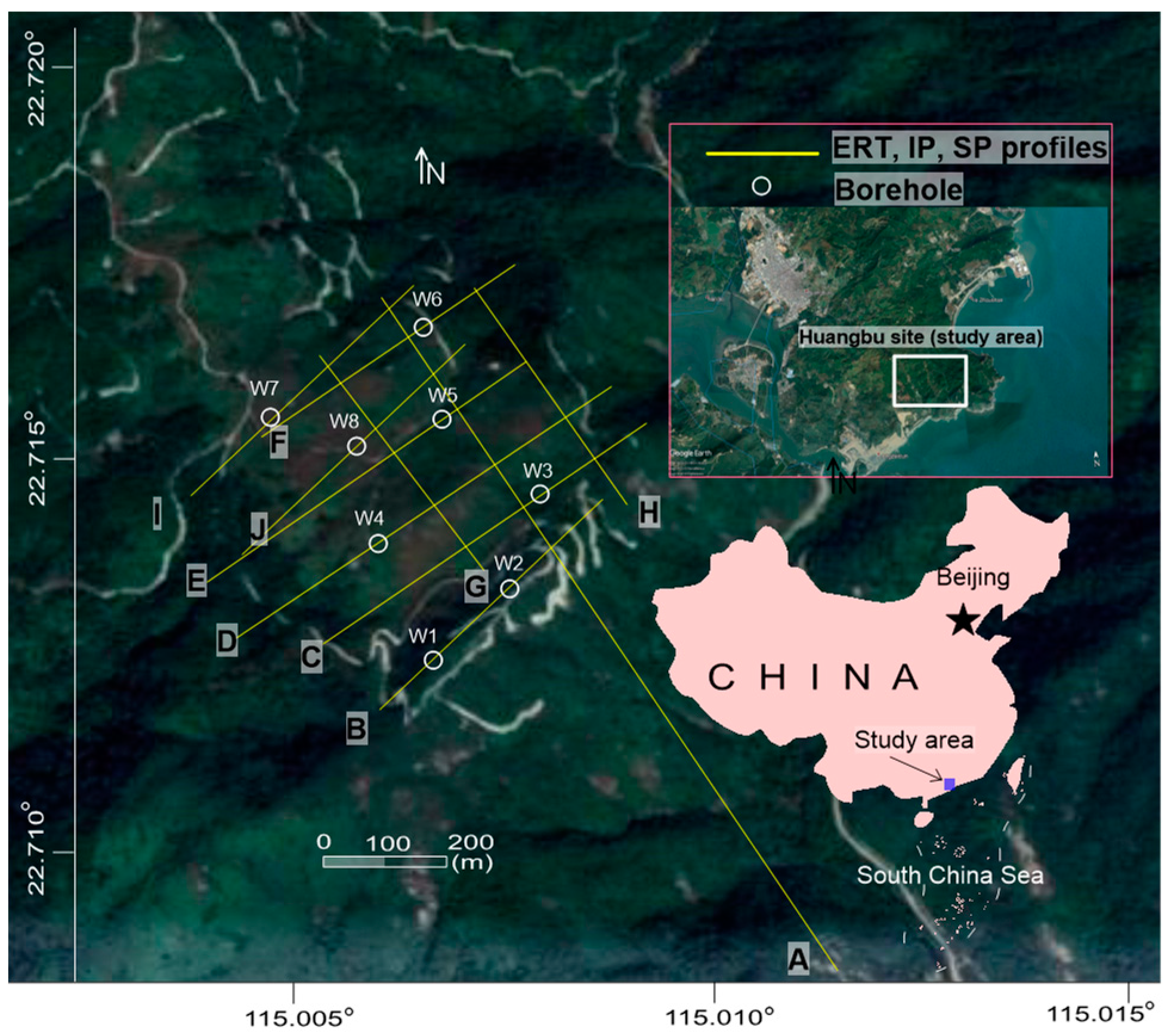
2. Study Area and Hydrogeology

The projected area is located in Huangbu, a coastal area of the South China Sea in Guangdong province of China (Figure 1). This investigation is a part of the project conducted by the Institute of Geology and Geophysics, Chinese Academy of Sciences to assess the hard-rock site for the development of engineering structures, such as facilities, laboratories and accelerator-driven systems. The investigated site is located in the Huidong Mountain Ranges including a tributary of Kaozhouyang River in northeast. The simplified geological settings of Huangbu consist of several localized faults, an unconformable boundary between the volcanic acidic rocks of Upper Jurassic and the magmatic/granite rocks of Lower Jurassic, and dynamo metamorphic zones [33]. Tuff rocks are dominant throughout the study area. The project area has a tropical climate system with the monsoon (rainy) season between May and September. The annual mean precipitation is 1950 mm [33]. Huangbu faces natural hazards, such as frequent typhoons, earthquakes and landslides, etc., [10]. It has a long summer with a maximum temperature of 40 °C and a short winter with a minimum temperature of 5 °C. The geological processes, such as weathering, tectonic and hydrothermal processes mainly cause fracturing in the study area [3]. The excess rainwater enters the fractures/discontinuities and makes the aquifer system. Groundwater resources are found within the weathered rock lying between the topsoil layer and the unweathered rock. Therefore, the delineation of weathered and unweathered rock, clay, and faults is the main challenge prior to the construction of engineered structures.

3. Materials and Methods

In the past decades, ERT has been widely used to assess hard-rock sites for the evaluation of weathered and unweathered layers, discontinuities, joints and fractures/faults [3,7,10,18,19,21,22,34,35]. It has been highly efficient in the areas dominated by the hydrogeological significance of weathering processes [9,10]. In ERT surveys, electrical resistivity is measured (in Ωm), which depends on the subsurface variations mainly associated with the type of rock, fractures, joints, lithology, water content, porosity, and permeability [3,36]. ERT data is collected using different electrode configurations which provide different resolutions [36]. ERT is affected by lithology and electrolytic conduction related to the size and configuration of the pore space, which is dependent on the size and shape of subsurface grains [9]. In general, electrical resistivity decreases with increasing water and clay content [37]. The resistivity of metamorphic and igneous rocks is higher than that of sedimentary rocks; similarly, the resistivity of unweathered rocks is higher than that of weathered/fractured rocks [10]. Thus, a huge contrast between resistivity values of weathered and unweathered rock is useful for the site suitability of the engineered structures [3,9]. ERT surveys are performed by injecting electric current into the subsurface via a pair of current electrodes, and the potential difference is measured through a pair of potential electrodes. The spacing between the electrodes controls the subsurface volume/area of influence. As the electrode spacing increases, the volume/area increases. The electrical resistivity measured in the field is known as the apparent resistivity (ρa) and is equal to:

$$\rho \mathrm{a}=\frac{KV}{I}$$

(1)

where V is the potential difference obtained between two potential electrodes, I is the direct electric current injected through two current electrodes, and K is the geometric factor that depends on the electrode spacings used to collect resistivity measurements. The electrical resistivity measured in the field does not show the true resistivity of the subsurface layers [10,38]. The apparent resistivity assumes a homogeneous subsurface. To solve for the true resistivity, apparent resistivities must be inverted [3,37].

IP is a method in which the subsurface materials get polarized as a result of the injection of an electric current into the subsurface [39,40]. Chargeability (in ms) is measured in the time-domain IP surveys. The electric field causes ions to displace within the EDL (electrical double layer). For time-domain IP, the measurement is the signal decay where displaced ions return back to the original state [41]. IP measurements are affected by the electrolyte properties in pore spaces, size of the grain, type of minerals, surface-water interaction, and the ratio of internal surface area to volume [42]. IP has higher polarization values for clay, sulfides and graphite; whereas its low values suggest the water content associated with the weathered/fractured zones in the hard rock terrains [30,31]. Thus, IP measurements have been very successful to differentiate between clay (with high chargeability and low resistivity) and weathered/fractured rock saturated with water (for low chargeability and low resistivity) [3]. In this investigation, IP was used as a supporting method of ERT to differentiate between water and clay.

SP is a passive geoelectrical technique, which measures natural potential (in mV) between two points on the ground [43]. SP anomalies are sensitive to the streaming potentials (e.g., groundwater flow). The high potential anomalies are mainly caused by conductive minerals, magnetite, sulfide ore bodies, graphite and groundwater flow [44,45,46]. SP anomalies at this site are mainly controlled by groundwater flow through the weathered/fractured zones [47]. The SP surveys measure positive and negative anomalies depending on the subsurface materials properties [48,49]. The groundwater flow system is mainly associated with negative SP anomalies [9]. In order to map the groundwater flow path in the study area, the SP measurements were obtained along with the ERT and IP data

Geophysical data acquisition of ERT, IP and SP was performed along the same profile using the same (constant) electrode spacing and the same number of measurements. All electrodes are connected to the resistivity meter via multi-core cables. The lateral and vertical resolution of the subsurface depends on the spacing between the electrodes. The resolution of a model increases with decreasing electrode spacing; however, this will reduce the depth of investigation. Therefore, electrode spacing should be selected considering a balance between the investigation depth and model resolution. The ERT, IP and SP data were obtained by the ABEM Lund Imaging System (ABEM Terrameter (SAS 4000)) along with ten profiles (A, B, C, D, E, F, G, H, I, and J) (Figure 1). A power amplifier, receiver and transmitter are all integrated into the imaging system. The system, connected with a PC, collects the main survey parameters including injected electric current, voltage, apparent resistivity, chargeability and self-potential. The ERT, IP and SP measurements were obtained using non-polarizing electrodes. Such electrodes are a requirement for IP and SP surveys to reduce contact resistances in electrically resistive mediums. A measurement of apparent resistivity, chargeability, and self-potential is performed for each electrode combination. This reading is displayed on the computer output at the lateral midpoint of the electrode locations and a prescribed depth level. Three parameters (electrical resistivity, chargeability and self-potential) are acquired at each of these points. First, the ERT data were obtained via Imaging System on resistivity mode. Afterwards, IP and SP measurements were obtained by using the Imaging System on IP and SP modes, respectively. The geophysical measurements (ERT, IP and SP) were acquired using the pole-dipole array with 5 m electrode spacing. The asymmetrical nature of this array was removed via the integration of two independent measurements (forward and reverse). Geophysical data of ERT, IP and SP along ten profiles were acquired for a total of 6150 m profile length, 1240 electrodes and 31,000 measurements, including 25 layers (depth levels) along each profile with the first layer at 7.5 m depth and last layer at 127.5 m depth. Data acquisition parameters of ERT, IP and SP along each profile are given in

Table 1. Data acquisition parameters of geophysical survey (ERT, IP and SP) including profile name, total number of electrodes for each profile, total profile length, electrode spacing along each profile, depth of first layer, depth of last layer, total layers (depth levels), and total number of measurements.

Profile	Electrodes	Profile Length (m)	Electrode Spacing (m)	1st Layer Depth (m)	Last Layer Dept (m)	Layers	Measurements
A	261	1300	5	7.5	127.5	25	6525
B	101	500	5	7.5	127.5	25	2525
C	111	550	5	7.5	127.5	25	2775
D	141	700	5	7.5	127.5	25	3525
E	111	550	5	7.5	127.5	25	2775
F	121	600	5	7.5	127.5	25	3025
G	111	550	5	7.5	127.5	25	2775
H	81	400	5	7.5	127.5	25	2025
I	101	500	5	7.5	127.5	25	2525
J	101	500	5	7.5	127.5	25	2525

. Prior to exporting geoelectrical data (apparent resistivity, chargeability and self-potential) to an inversion package, PROSYSII (IRIS Instruments) was used to display raw data in graphical plots, and to separate and remove incorrect data points (low/very high potential readings compared with surrounding readings). Furthermore, the signal strength was also enhanced through the use of stacking, i.e., the repeated measurement of transfer resistance through a number of cycles of current injection. The geophysical data obtained in the field were further processed. The apparent electrical resistivity, IP and assigned data weights were inverted by RES2DINV [37]. ZondSP2D program was used for SP data inversion. In SP inversion, the medium model is created through a number of cells, and each cell has the electrical value and type of conductivity (ion or electronic) properties. RES2DINV provides the 2D resistivity/IP model via the nonlinear optimization procedure [37,50]. The robust constraint was used to enhance the data quality by removing the bad data (data values that cause spikes when compared with the surrounding data points and/or data with standard deviations over the average). Thus, the fit of the data to the model can be improved through filtering or using higher standard deviation weights on bad data. A standard deviation weight measures the dispersion of values when some values have higher weights than others. Data weights determine reciprocal errors which provide a measure of the error caused by an instrument, natural electrical storms and nearby anthropogenic current sources. RES2DINV uses the smoothness-constrained least squares inversion with L2-norm. The inversion program minimized the root mean square error (RMS) up to 5%. RMS is calculated as the square of the difference obtained between the estimated and observed apparent resistivity. The ERT models were generated within three to five iterations. The standard technique of Gauss Newton optimization was used in the inversion program. The inversion method was performed using a low damping factor of 0.03.

4. Results and Discussion

Geophysical data of three methods (ERT, IP and SP) were used to interpret the subsurface for site suitability of engineered structures in the study area. The subsurface was interpreted for the delineation of distinct layers, fractures/faults, clay, and groundwater flow path. 2D ERT models were integrated with the borehole lithological logs to obtain a subsurface model of four distinct layers/zones with specific resistivity values range. Clay was identified by the integration of 2D IP models (with high chargeability) and 2D ERT models (with low resistivity). Groundwater flow was mapped using 2D SP models (with low or negative SP). The main fractures/faults were delineated by the integration of all geophysical models using low values of ERT, IP and SP. One of the interpreted models for three geophysical methods is shown in Figure 2. Based on the correlation between all ERT models and borehole data, the ERT model (Figure 2a) along profile B was interpreted (Figure 2b) for four layers (topsoil cover, weathered layer, weathered/unweathered transition zone (partly weathered rock) and unweathered layer) and four main fractures/faults (F2, F3, F4 and F5). The identified fractures/faults in ERT B also show consistency on IP B (Figure 2c) and SP B model (Figure 2d). The ambiguity in the water-clay distinction caused by low resistivity in the ERT model (Figure 2a) was removed by integration of IP (with high chargeability) (Figure 2c). Similarly, negative SP shows the direction of groundwater flow mainly along the identified fractures/faults (Figure 2d). The details of subsurface interpretation for all geophysical profiles are given in the following sections.

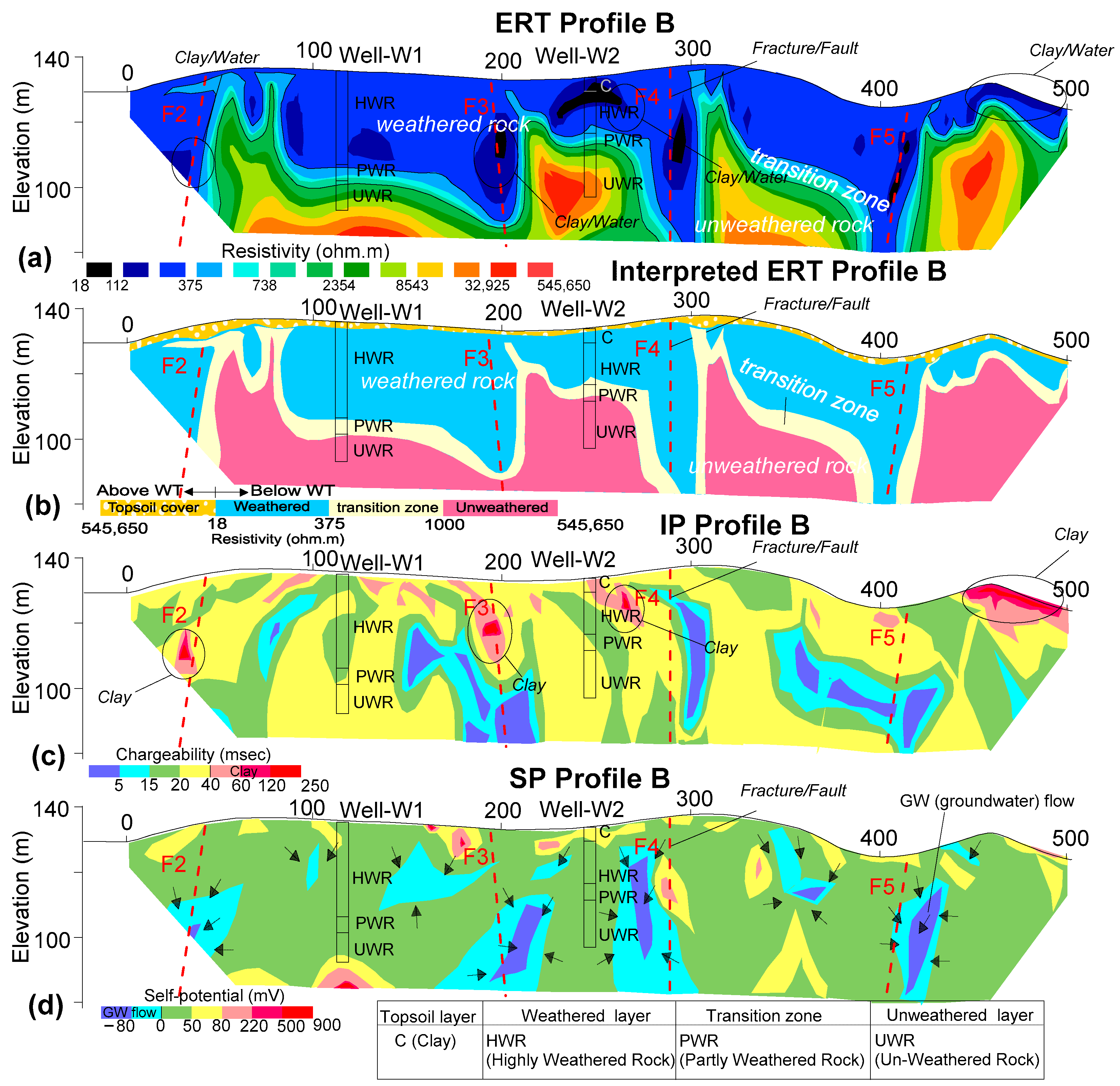
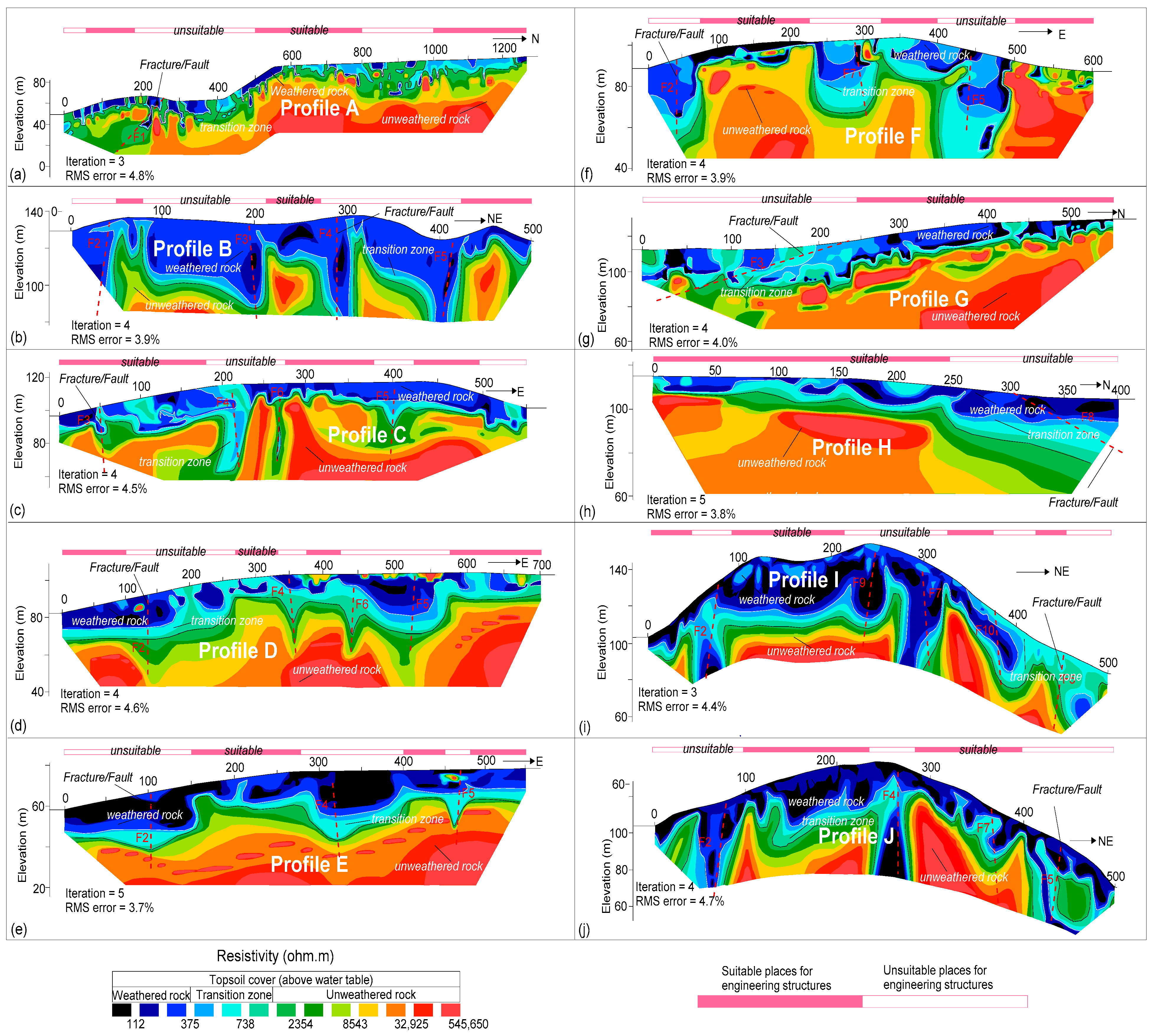
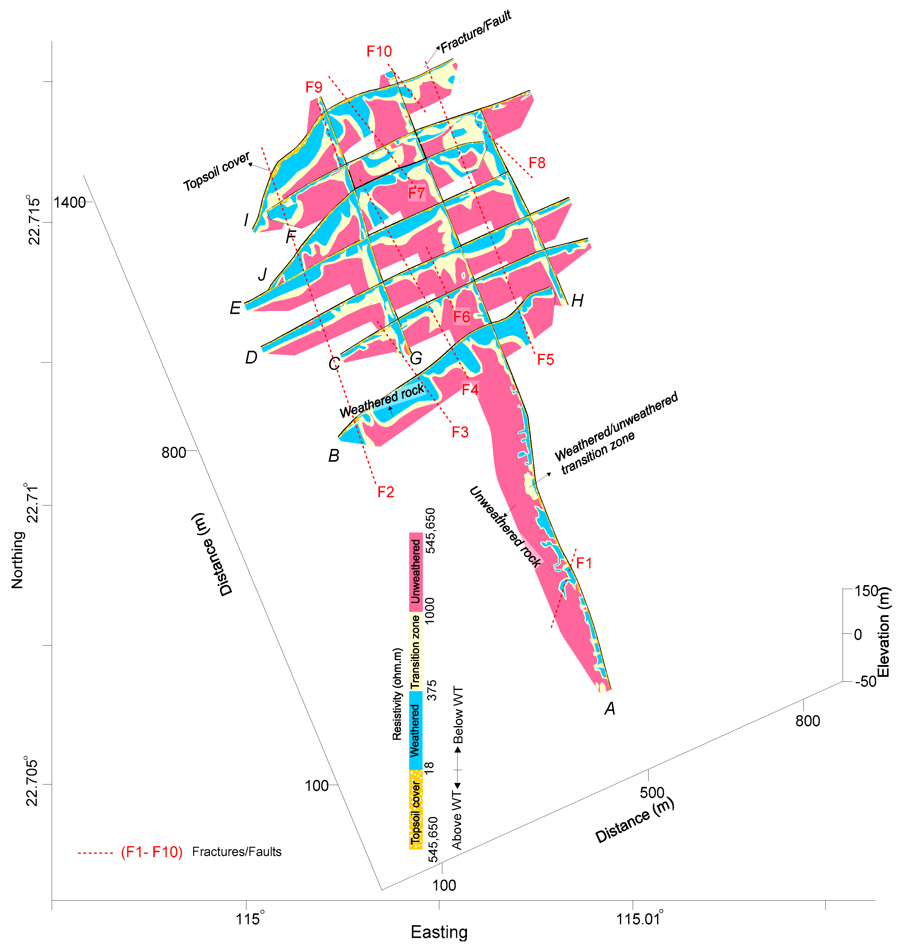
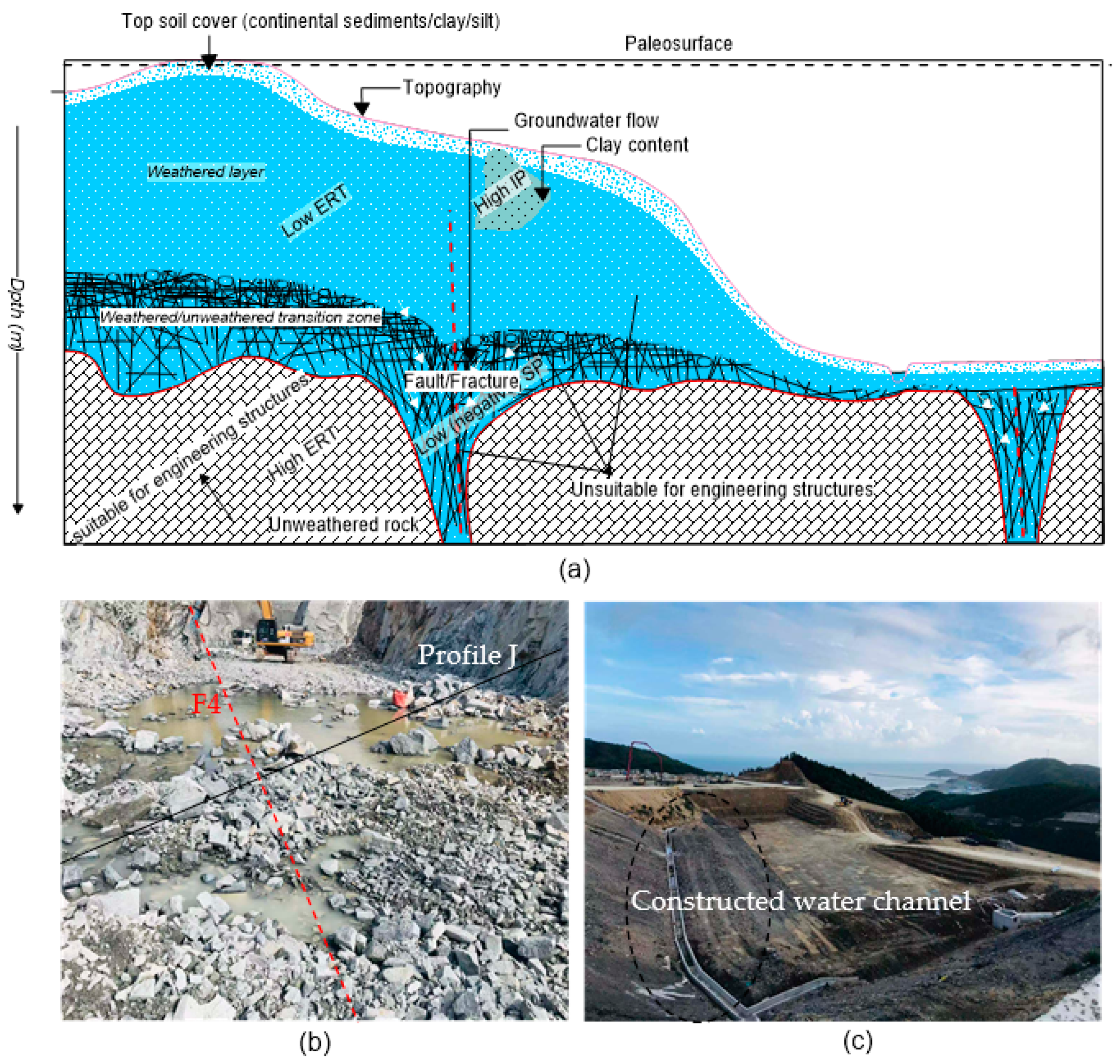
4.1. Delineation of Subsurface Layers

The 2D ERT models along with all profiles generated by the inversion program of RES2DINV are shown in Figure 3. The electrical resistivity varies between 18–545,650 Ωm along all ERT profiles over the entire investigated site. Based on the correlation between ten ERT models and the local hydrogeological information obtained by eight boreholes, the interpretation was constrained for a four-layered model of topsoil cover, weathered layer (highly weathered rock), weathered/unweathered transition zone (partly weathered rock) and unweathered layer. The topsoil cover of dry strata above the water table was delineated with a resistivity less than 180,500 Ωm, the weathered layer below the water table underlying the top layer was evaluated with a resistivity between 18–375 Ωm, the unweathered rock at the bottom was revealed with a resistivity greater than 1000 Ωm and as high as 545,650 Ωm, and the transition zone between weathered and unweathered layer (below the water table) was identified with resistivity ranging from 375 to 1000 Ωm. The weathered layer, unweathered layer and weathered/unweathered transition zone (partly weathered layer) are clearly identified in 2D ERT models shown in Figure 3.

All 2D ERT profiles were integrated and interpreted for the delineation of weathered layer, weathered/unweathered transition zone and unweathered rock as shown in Figure 4. Thus, a 3D view of the integrated 2D ERT profiles provides a clearer view of the subsurface layers over the entire area. Each ERT model in Figure 3 and Figure 4 was interpreted for the identification of the most suitable places for the construction of engineering structures. Average depth/thickness of the delineated topsoil cover, unweathered layer, weathered/unweathered transition zone and weathered layer, including most appropriate locations for engineering construction along each profile are given in

Table 2. Results obtained from the interpreted ERT models suggesting the most suitable places for the construction of engineering structures, including average thickness/depth of the topsoil layer, weathered layer, weathered/unweathered transition zone and unweathered layer along each profile.

Profile	Average Depth/Thickness of Subsurface Layers				Most Suitable Places for Engineering Structures (m)
	Topsoil Thickness (m)	Weathered Layer Thickness (m)	Transition Zone Thickness (m)	Unweathered Layer Depth (m)
A	3	10	7	20	60–180, 500–800, 1000–1300
B	3	26	6	35	50–75, 220–275, 430–500
C	3	10	7	20	0–175, 275–375, 425–490
D	3	10	9	22	0–100, 275–325, 375–425, 575–700
E	2	11	7	20	150–275, 400–450, 480–550
F	3	16	13	32	75–225, 325–400, 500–600
G	3	11	6	20	240–550
H	2	8	8	18	0–250
I	5	15	10	30	0–50, 90–210, 325–375, 430–450
J	3	16	11	30	100–225, 290–400

. Results of ten ERT models in Table 2 reveal that the topsoil cover is evaluated with an average depth of 3 m, the weathered layer is evaluated with an average thickness of 14 m, the weathered/unweathered transition zone (partly weathered rock) is interpreted with an average thickness of 8 m, and the unweathered layer is delineated at an average depth of 25 m. The results suggest that ERT profiles A, G and H are more suitable for engineering construction compared with other profiles since they reveal only one deep weathered/transition zone and lower thickness of the weathered rock; while profiles profile B, F, I and J provide the most unsuitable places for construction as they delineate several deep weathered/transition zones and thick weathered layer. Looking at the ERT results alone, the southeastern parts of the project area provide more suitable places for engineering structures due to a shallower depth to the unweathered zone.

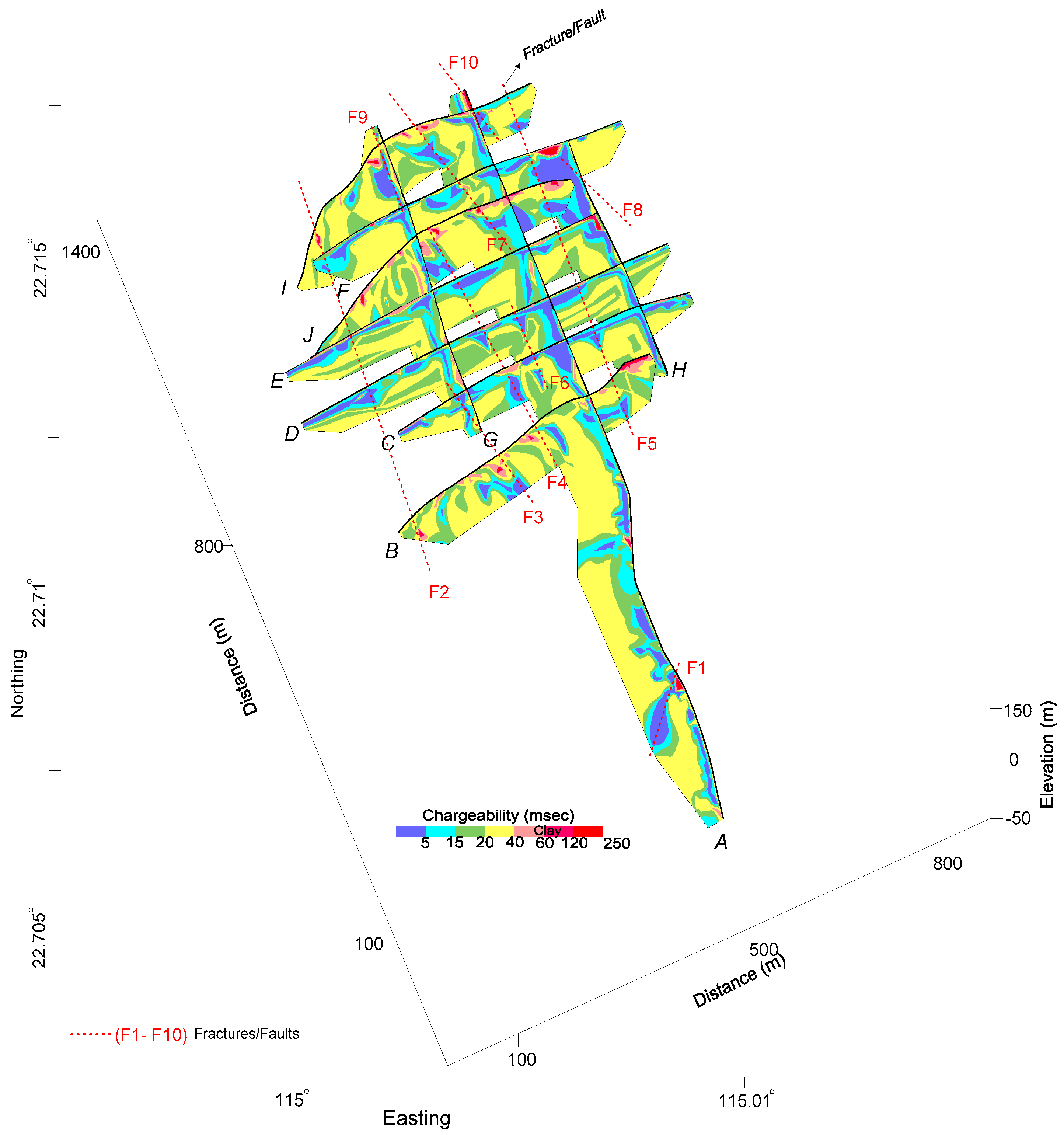
4.2. Detection of Faults

Low resistive zones (resistivity less than 1000 Ωm) were interpreted either as a weathered layer or the fracture/fault. A total of ten main fractures/faults (F1–F10) were delineated over the entire investigated site (Figure 4). These faults were interpreted based on the hydrogeological information of the study area, the deep weathered zones and an overall model generated by the integration of all ERT models (Figure 4). The identified fractures/faults provide the most unsuitable foundation rock for engineering design. Along profile A, one fault (F1) was detected at 220 m distance. Profile B revealed four faults, such as F2 at 30 m, F3 at 190 m, F4 at 280 m and F5 at 400 m distance. Profile C evaluated four faults, such as F3 at 50 m, F4 at 210 m, F6 at 270 m and F5 at 400 m distance. Profile D revealed four faults, such as F2 at 130 m distance, F4 at 350 m, F6 at 450 m, and F5 at 530 m distance. Profile E detected three faults, such as F2 at 120 m, F4 at 310 m and F5 at 470 m distance. Three faults were identified along profile F, such as F2 at 40 m distance, F7 at 290 m, and F5 at 440 m distance. Along profile G, one fault (F3) was identified at a distance of 120 m. One fault F8 was revealed along profile H in the north at 350 m distance. Along profile I, five faults were detected, such as F2 at 70 m, F9 at 250 m, F7 at 300 m, F10 at 390 m, and F5 at 470 m distance. Similarly, four faults were evaluated along profile J, such as F2 at 70 m, F4 at 270 m, F7 at 370 m and F5 at 450 m distance. F1 with the northeast-southwest direction was identified along profile A in the south. The overall orientation of faults F2–F10 is from northwest to southeast. F2 and F5 are the longest faults with about 700 m in length. F1, F6, F8, F9 and F10 are the shortest faults with lengths of about 150 m. Whereas F3, F4 and F7 are about 300–550 m long. The fractures/faults were identified by low values of resistivity (Figure 2a), IP (Figure 2c) and SP (Figure 2d).

4.3. Water-Clay Distinction

Electrical resistivity obtained from ERT models cannot distinguish between clay and weathered rock saturated with water, since low resistivity suggests water as well as clay. Thus, ERT models alone cause ambiguity in the interpretation of the subsurface geological model. On the other hand, high IP suggests a higher likelihood of clays while low IP suggests fluid-filled voids. Therefore, such uncertainty in the model was removed by the integration of ERT and IP. Based on the integration between ERT and IP models, and the borehole information, clay was identified with IP greater than 40 ms and resistivity less than 1000 Ωm. The results suggest that mostly clay was delineated along the fractures/faults near the surface (Figure 5). The prominent clay content along profile A was delineated at 220 m, 490 m, 1000 m and 1300 m. Clay was identified at four places along profile B, such as at 30 m, 190 m, 280 m and 480 m distance. Profile C revealed clay at three locations, such as at 40 m, 210 m and 520 m distance. Profile D revealed thin clay content at several places near the surface. Profile E detected the high clay content at 550 m on the east side. The main clay content along profile F was revealed at a 500 m distance. Along profile G, minor clay content was identified at a 75 m distance. Along profile H, two places of high clay were identified at the integration of profiles E and F. Along profile I, clay was detected at four places, at 70 m, 250 m, 300 m and 390 m distance. Compared with other profiles, mostly the topsoil layer in profile J is dominant with clay, especially along the fractures/faults. The locations identified by clay may cause the collapse of the engineered structures. Therefore, clay identified along the 2D IP profiles should be avoided in the construction.

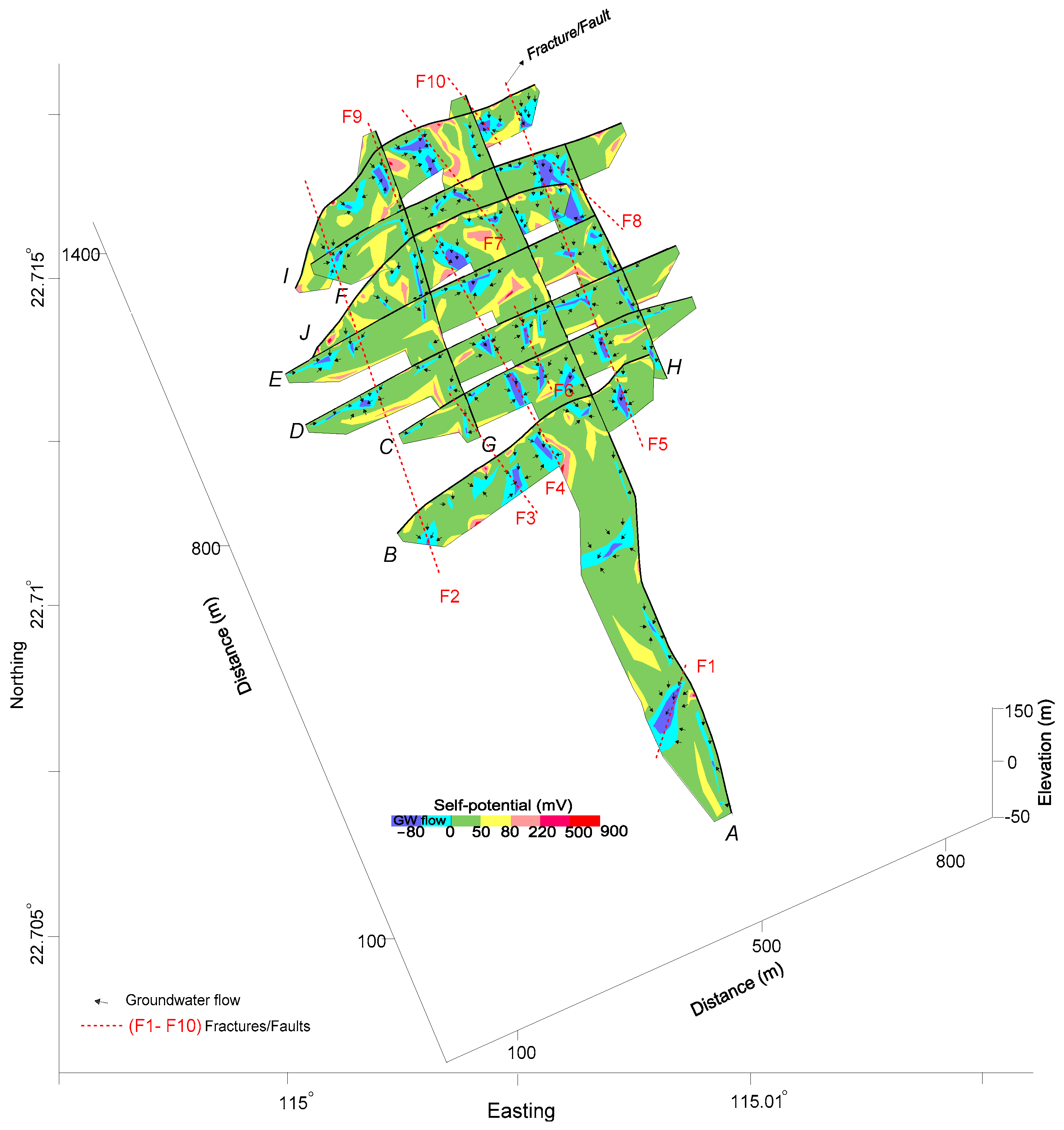
4.4. Groundwater Flow Modeling

Most of the uncertainties in the subsurface geological model were reduced/removed by 2D ERT and IP models through the delineation of weathered and unweathered rock, detection of fractures/faults, and the distinction between water and clay. However, ERT and IP cannot map the groundwater flow in the investigated area. Groundwater flow mapping was performed by SP. SP anomalies suggest both positive and negative values ranging from −150 mV to 900 mV over the entire investigated area. The negative SP suggests the groundwater flow path. The 2D SP models were generated along the same ERT and IP profiles. The 2D SP models interpreted for the groundwater flow are shown in Figure 6. The integration of 2D SP models provides an overall view of the projected site with clear insights into the subsurface. The SP results suggest that the groundwater flow is mainly mapped along the main fractures/faults. The arrowheads in Figure 6 suggest the groundwater flow direction. Furthermore, the low SP (negative values) delineates the fractures/faults. Hence, in addition to the groundwater flow mapping, SP also supports ERT and IP for the delineation of fractures/faults, and hence the accuracy in the interpretation of the subsurface geological model is increased. The results obtained by different geophysical methods show a good correlation with each other and the hydrogeological information of the project site (Figure 2, Figure 3, Figure 4, Figure 5 and Figure 6). Thus, the use of integrated geophysical methods reduces the geological model uncertainties caused by the limited data and provides more accuracy in the subsurface geological model for the successful construction of engineered structures.

Based on the interpretation of the subsurface using three geophysical methods, a conceptual model of the investigated site was obtained as shown in Figure 7a. The conceptual model provides an overall picture of the study area for the delineation of four distinct layers (topsoil cover, weathered layer, weathered/unweathered transition zone and unweathered layer using ERT, the main faults using ERT, IP and SP, clay using ERT and IP, and groundwater flow path using SP.

5. Conclusions

In this work, we used an integrated approach of three geophysical methods namely electrical resistivity tomography (ERT), induced polarization (IP) and self-potential (SP). We used this geophysical approach to assess a highly heterogeneous site in South China for the successful construction of the engineered structures. Traditionally, drilling tests are conducted to get the subsurface geological information. However, such tests suffer limitations in terms of cost, coverage and topographic constraints, etc. Furthermore, it may not be possible for planners to drill a large number of wells that provide the point measurements vertically. On the other hand, geophysical methods are non-invasive, cheaper, and provide subsurface geological knowledge both laterally and vertically. Such methods can be integrated with the available geological information obtained from the limited boreholes in order to investigate the large area entirely.

In this work, we calibrated ERT with the local geological information of eight boreholes and constrained the subsurface into four discrete layers with specific values range of resistivities, such as the topsoil layer above water table with a resistivity between 18–180,500 Ωm, the weathered layer with resistivity ranging from 18 and 375 Ωm, the weathered/unweathered transition zone (partly weathered rock) with resistivity ranging from 375 to 1000 Ωm, and the unweathered layer with a resistivity between 18–545,650 Ωm. The interpreted 2D ERT models delineated the subsurface layers over the entire area, such as the topsoil layer with an average thickness of 3 m, the weathered layer with an average thickness of 14 m, transition zone with an average thickness of 8 m, and the unweathered layer at an average depth of 25 m. IP was integrated with ERT to delineate clay since ERT alone cannot differentiate between water and clay because low resistivity shows either clay or water. Clay was identified with chargeability greater than 40 ms and resistivity less than 1000 Ωm. The deep weathered zones were delineated as the main faults and localized fractures in the project site. Our observation suggests that low values of geophysical parameters (resistivity and chargeability) suggest the faults/fractures saturated with water, such as ERT less than 1000 Ωm, IP less than 15 ms and SP less than 0 mV. Groundwater flow along the faults/fractures was mapped by SP. Negative SP mapped the groundwater accumulation mainly along the faults/fractures. Based on the results of ERT, IP and SP, we recommend the most suitable places for the development of engineering structures along each profile (Table 2). Our findings will help the site engineers with the accurate design of engineering structures in the investigated area. Results of this study including the conceptual model (Figure 7a) will also be useful for the interpretation of nearby sites. Our results were confirmed by the actual situation of the investigated site during the construction, such as groundwater seepage during the site construction was clearly observed from the identified fractures/faults (Figure 7b), and the construction design was modified based on our geophysical results (Figure 7c). Our approach of integrated geophysical methods provides better insights into the subsurface for the construction of engineering structures in highly heterogeneous hard rock terrains.

References

1. Fan, X.M.; Xu, Q.; Zhang, Z.Y.; Meng, D.S.; Tang, R. The genetic mechanism of a translational landslide. Bull. Eng. Geol. Environ. 2009, 68, 231–244. [Google Scholar] [CrossRef]
2. Li, K.; Shang, Y.; He, W.; Lin, D.; Hasan, M.; Wang, K. An engineering site suitability index (ESSI) for the evaluation of geological situations based on a multi-factor interaction matrix. Bull. Eng. Geol. Environ. 2017, 78, 569–577. [Google Scholar] [CrossRef]
3. Hasan, M.; Shang, Y.; Jin, W.; Akhter, G. An engineering site investigation using non-invasive geophysical approach. Environ. Earth Sci. 2020, 79, 265. [Google Scholar] [CrossRef]
4. Asch, T.W.J.V.; Hendriks, M.R.; Hessel, R.; Rappange, F.E. Hydrological triggering conditions of landslides in varved clays in the French Alps. Eng. Geol. 1996, 42, 239–251. [Google Scholar] [CrossRef]
5. Hongbin, L.V.; Chengpeng, L.; Bill, X.H.; Jiaxin, R.; Yanan, Z.; Qiang, X.; Juxiu, T. Characterizing groundwater flow in a translational rock landslide of southwestern China. Bull. Eng. Geol. Environ. 2017, 78, 3223–3237. [Google Scholar] [CrossRef]
6. Ayodele, Y.G.; Joshua, A.O.; Sunday, O.J. An Engineering Site Characterization using Geophysical Methods: A Case Study from Akure, Southwestern Nigeria. J. Earth Sci. Geotech. Eng. 2015, 5, 57–77. [Google Scholar]
7. Wyns, R.; Baltassat, J.M.; Lachassagne, P.; Legchenko, A.; Vairon, J.; Mathieu, F. Application of Magnetic Resonance Soundings to Groundwater Reserves Mapping in Weathered Basement Rocks (Brittany, France). Bull. Soc. Géol. Fr. 2002, 175, 21–34. [Google Scholar] [CrossRef]
8. Taylor, R.; Howard, K. A tectono-geomorphic model of the hydrogeology of deeply weathered crystalline rock: Evidence from Uganda. Hydrogeol. J. 2000, 8, 279–294. [Google Scholar] [CrossRef]
9. Gao, Q.; Shang, Y.; Hasan, M.; Jin, W.; Yang, P. Evaluation of a Weathered Rock Aquifer Using ERT Method in South Guangdong, China. Water 2018, 10, 293. [Google Scholar] [CrossRef] [Green Version]
10. Hasan, M.; Shang, Y.; Jin, W. Delineation of weathered/fracture zones for aquifer potential using an integrated geophysical approach: A case study from South China. J. Appl. Geophys. 2018, 157, 47–60. [Google Scholar] [CrossRef]
11. Guoxing, C.; Jiao, Z.; Mengyun, O.; Wenping, G. Three- dimensional site characterization with borehole data-A case study of Suzhou area. Eng. Geol. 2018, 234, 65–82. [Google Scholar]
12. Shang, Y.J.; Yang, C.G.; Jin, W.J.; Chen, Y.W.; Hasan, M.; Wang, Y.; Li, K.; Lin, D.M.; Zhou, M. Application of Integrated Geophysical Methods for Site Suitability of Research Infrastructures (RIs) in China. Appl. Sci. 2021, 11, 8666. [Google Scholar] [CrossRef]
13. Sikandar, P.; Christen, E.W. Geoelectrical sounding for the estimation of hydraulic conductivity of alluvial aquifers. Water Resour. Manag. 2012, 26, 1201–1215. [Google Scholar] [CrossRef]
14. Chang, L.C.; Ho, C.C.; Yeh, M.S.; Yang, C.C. An integration approach for conjunctive-use planning of surface and subsurface water system. Water Resour. Manag. 2011, 25, 29–78. [Google Scholar] [CrossRef]
15. Bianchi, G.; Fasani Bozzano, F.; Cardarelli, E.; Cercato, M. Underground cavity investigation within the city of Rome (Italy): A multi-disciplinary approach combining geological and geophysical data. Eng. Geol. 2013, 152, 109–121. [Google Scholar] [CrossRef]
16. Suzuki, K.; Toda, S.; Kusunoki, K.; Fujimitsu, Y.; Mogi, T.; Jomori, A. Case studies of electrical and electromagnetic methods applied to mapping active faults beneath the thick quaternary. Eng. Geol. 2000, 56, 29–45. [Google Scholar] [CrossRef]
17. Kneisel, C. Assessment of subsurface lithology in mountain environments using 2D resistivity imaging. Geomorphology 2006, 80, 32–44. [Google Scholar] [CrossRef]
18. Cardarelli, E.; Cercato, M.; Di Filippo, G. Assessing foundation stability and soil structure interaction through integrated geophysical techniques: A case history in Rome (Italy). Near Surf. Geophys. 2007, 59, 244–259. [Google Scholar] [CrossRef]
19. Chambers, J.C.; Kuras, O.; Meldrum, P.I.; Ogilvy, R.D.; Hollands, J. Electrical resistivity tomography applied to geologic, hydrologic and engineering investigations at a former waste disposal site. Geophysics 2006, 71, B231–B239. [Google Scholar] [CrossRef] [Green Version]
20. Martinez, J.; Mendoza, R.; Rey, J.; Sandoval, S.; Hidalgo, M.C. Characterization of Tailings Dams by Electrical Geophysical Methods (ERT, IP): Federico Mine (La Carolina, Southeastern Spain). Minerals 2021, 11, 145. [Google Scholar] [CrossRef]
21. Kim, J.H.; Yi, M.J.; Song, Y.; Seol, S.J.; Kim, K.S. Application of geophysical methods to the safety analysis of an earth dam. J. Environ. Eng. Geophys. 2007, 12, 221–235. [Google Scholar] [CrossRef]
22. Osinowo, O.O.; Akanji, A.O.; Akinmosin, A. Integrated geophysical and geotechnical investigation of the failed portion of a road in Basement Complex terrain, southwestern Nigeria. RMZ—Mater. Geoenviron. 2011, 58, 143–162. [Google Scholar]
23. Lghoul, M.; Teixido, T.; Pena, J.A.; Hakkou, R.; Kchikach, A.; Guerin, R.; Jaffal, M.; Zouhri, L. Electrical and Seismic Tomography Used to Image the Structure of a Tailings Pond at the Abandoned Kettara Mine, Morocco. Int. J. Mine Water 2012, 31, 53–61. [Google Scholar]
24. Loperte, A.; Soldovieri, F.; Palombo, A.; Santini, F.; Llapenna, V. An integrated geophysical approach for water infiltration detection and characterization at Monte Cotugno rock-fill Dam (southern Italy). Eng. Geol. 2016, 211, 162–170. [Google Scholar] [CrossRef]
25. Samyn, K.; Mathieu, F.; Bitri, A.; Nachbaur, A.; Closset, L. Integrated geophysical approach in assessing karst presence and sinkhole susceptibility along flood-protection dykes of the Loire River, Orléans, France. Eng. Geol. 2014, 183, 170–184. [Google Scholar] [CrossRef] [Green Version]
26. Lin, C.H.; Lin, C.P.; Hung, Y.C.; Chung, C.C.; Wu, P.L.; Liu, H.C. Application of geophysical methods in a dam project: Life cycle perspective and Taiwan experience. J. Appl. Geophys. 2018, 158, 82–92. [Google Scholar] [CrossRef]
27. Kukemilks, K.; Wagner, J.F. Detection of Preferential Water Flow by Electrical Resistivity Tomography and Self-Potential Method. Appl. Sci. 2021, 11, 4224. [Google Scholar] [CrossRef]
28. Hung, Y.C.; Chou, H.S.; Lin, C.P. Appraisal of the Spatial Resolution of 2D Electrical Resistivity Tomography for Geotechnical Investigation. Appl. Sci. 2020, 10, 4394. [Google Scholar] [CrossRef]
29. Hasan, M.; Shang, Y.; Jin, W.; Akhter, G. Investigation of fractured rock aquifer in South China using electrical resistivity tomography and self-potential methods. J. Mt. Sci. 2019, 16, 850–869. [Google Scholar] [CrossRef]
30. Revil, A.; Murugesu, M.; Prasad, M.; Le Breton, M. Alteration of volcanic rocks: A new non-intrusive indicator based on induced polarization measurements. J. Volcanol. Geotherm. Res. 2017, 341, 351–362. [Google Scholar] [CrossRef]
31. Johnson, T.C.; Versteeg, R.J.; Ward, A.F.; Day-Lewis, D.; Revil, A. Improved hydrogeophysical characterization and monitoring through high performance electrical geophysical modeling and inversion. Geophysics 2010, 75, WA27–WA41. [Google Scholar] [CrossRef]
32. Jardani, A.; Revil, A.; Barrash, W.; Crespy, A.; Rizzo, E.; Straface, S.; Cardiff, M.; Malama, B.; Miller, C.; Johnson, T. Reconstruction of the water table from self potential data: A Bayesian approach. Groundwater 2009, 47, 213–227. [Google Scholar] [CrossRef]
33. Bureau of Geology and Mineral Resources of Guangdong Province. Regional Geology of Guangdong Province; Geology Publishing House: Beijing, China, 1988; pp. 1–602. (In Chinese)
34. Tejero, A.; Chávez, R.E.; Urbierta, J.; Flores-Márquez, E.L. Cavity detection in the southwestern hilly portion of Mexico City by resistivity imaging. J. Environ. Eng. Geophys. 2002, 7, 130–139. [Google Scholar] [CrossRef]
35. Lech, M.; Skutnik, Z.; Bajda, M.; Markowska-Lech, K. Applications of Electrical Resistivity Surveys in Solving Selected Geotechnical and Environmental Problems. Appl. Sci. 2020, 10, 2263. [Google Scholar] [CrossRef] [Green Version]
36. Loke, M.H.; Acworth, I.; Dahlin, T. A comparison of smooth and blocky inversion methods in 2D electrical imaging surveys. Explor. Geophys. 2003, 34, 182–187. [Google Scholar] [CrossRef]
37. Loke, M.H.; Barker, R.D. Rapid least-squares inversion of apparent resistivity pseudosections by a quasi-Newton method. Geophys. Prospect. 1996, 44, 131–152. [Google Scholar] [CrossRef]
38. Loke, M.H.; Chambers, J.E.; Rucker, D.F.; Kuras, O.; Wilkinson, P.B. Recent developments in the direct-current geoelectrical imaging method. J. Appl. Geophys. 2013, 95, 135–156. [Google Scholar] [CrossRef]
39. Ward, S.H. Resistivity and Induced Polarization Methods in Geotechnical and Environmental Geophysics; Society of Exploration Geophysicists: Tulsa, OK, USA, 1990; pp. 147–190. [Google Scholar]
40. Routh, P.S.; Oldenburg, D.W. Electromagnetic coupling in frequency-domain induced polarization: A method for removal. Geophys. J. Int. 2001, 145, 59–76. [Google Scholar] [CrossRef]
41. Dahlin, T.; Leroux, V.; Nissen, J. Measuring Techniques in Induced Polarization Imaging. J. Appl. Geophys. 2002, 50, 279–298. [Google Scholar] [CrossRef] [Green Version]
42. Yuval; Oldenburg, D.W. Computation of Cole-Cole parameters from IP data. Geophysics 1997, 62, 436–448. [Google Scholar] [CrossRef] [Green Version]
43. Telford, W.M.; Geldarl, L.P.; Sheriff, R.E. Applied Geophysics; Cambridge University Press: Cambridge, UK, 1990. [Google Scholar]
44. Meisner, P. A method of qualitative interpretation of self potential measurements. Geophys. Prospect. 1962, 10, 203–218. [Google Scholar] [CrossRef]
45. Paul, M.K. Direct interpretation of self-potential anomalies caused by inclined sheets of finite horizontal extension. Geophysics 1965, 30, 418–423. [Google Scholar] [CrossRef]
46. Lowrie, W. Fundamentals of Geophysics; Cambridge University Press: Cambridge, UK, 1997. [Google Scholar]
47. Self Potential Technique. 2008. Available online: http://www.nga.com/Geo_ser_Self_potential_tech.htm (accessed on 20 July 2008).
48. Mitchell, J.K. Fundamentals of Soil Behavior; John Wiley and Sons: New York, NY, USA, 1976. [Google Scholar]
49. Corwin, R.F.; Hoover, D.B. The self potential method in geothermal exploration. Geophysics 1979, 44, 226. [Google Scholar] [CrossRef] [Green Version]
50. Griffiths, D.H.; Barker, R.D. Two-dimensional resistivity imaging and modeling in areas of complex geology. J. Appl. Geophys. 1993, 29, 211–226. [Google Scholar] [CrossRef]
Figure 1. Location of the investigated area including the geophysical profiles (yellow lines) of ERT, IP and SP measurements, and boreholes (white circles).
Applsci 11 10752 g001
Figure 2. (a) 2D ERT model along profile B, (b) 2D ERT model along the same profile B interpreted for subsurface layers and fractures/faults based on the correlation between ERT models and borehole lithological logs, (c) 2D IP model along the same profile B interpreted for clay and fractures/faults, and (d) 2D SP model along profile B interpreted for groundwater flow path and fractures/faults.
Applsci 11 10752 g002
Figure 3. (aj) 2D resistivity models of ERT (resistivity increasing from black to red on a color scale) along all geophysical profiles generated by the inversion program of RES2DINV. The zones marked by pink color on the top of each ERT model suggest suitable places for engineering structures, whereas the zones of white color indicate unsuitable locations for engineering structures.
Applsci 11 10752 g003
Figure 4. Integration of 2D ERT models along all profiles interpreted for the weathered rock (blue color), weathered/unweathered transition zone or partly weathered rock (yellow color) unweathered rock (pink color), and fractures/faults (dotted reds lines).
Applsci 11 10752 g004
Figure 5. Integration of 10 2D IP models along all profiles (with IP increasing from blue to red on a color bar) interpreted for the clay (shown by red color), and fractures/faults (dotted reds lines).
Applsci 11 10752 g005
Figure 6. Integration of 2D SP models along all profiles (with SP increasing from blue to red on a color bar) interpreted for the groundwater flow modeling (shown by black arrows) and the fractures/faults (dotted reds lines).
Applsci 11 10752 g006
Figure 7. (a) A four layered-conceptual model of the investigated area obtained using three geophysical methods (ERT, IP and SP) for the delineation of subsurface layers, fractures/faults, clay and groundwater flow, (b) Water seepage during the construction as identified by the interpreted fault F4 along profile J, and (c) A change in construction design was made by constructing a water channel for water infiltration from the identified faults/fractures on southwest side of the project site.
Applsci 11 10752 g007