Deep Learning and Internet of Things for Beach Monitoring: An Experimental Study of Beach Attendance Prediction at Castelldefels Beach

Abstract

Smart seaside cities can fully exploit the capabilities brought by Internet of Things (IoT) and artificial intelligence to improve the efficiency of city services in traditional smart city applications: smart home, smart healthcare, smart transportation, smart surveillance, smart environment, cyber security, etc. However, smart coastal cities are characterized by their specific application domain, namely, beach monitoring. Beach attendance prediction is a beach monitoring application of particular importance for coastal managers to successfully plan beach services in terms of security, rescue, health and environmental assistance. In this paper, an experimental study that uses IoT data and deep learning to predict the number of beach visitors at Castelldefels beach (Barcelona, Spain) was developed. Images of Castelldefels beach were captured by a video monitoring system. An image recognition software was used to estimate beach attendance. A deep learning algorithm (deep neural network) to predict beach attendance was developed. The experimental results prove the feasibility of Deep Neural Networks (DNNs) for beach attendance prediction. For each beach, a classification of occupancy was estimated, depending on the number of beach visitors. The proposed model outperforms other machine learning models (decision tree, k-nearest neighbors, and random forest) and can successfully classify seven beach occupancy levels with the Mean Absolute Error (MAE), accuracy, precision, recall and F1-score of 0.03, 92.7%, 92.9%, 92.7%, and 92.7%, respectively.

1. Introduction

The term smart city was first used in the 1990s for the use of Information and Communication Technologies (ICT) to develop modern infrastructures within cities [1]. Afterwards, the smart city concept evolved and is no longer limited to the diffusion of ICT, it is also related to people and community needs. Smart cities are cities that use ICT to develop new urban intelligence functions in such a way that community and quality of life are enhanced [2]. New decision-making paradigms have been developed for optimizing the continuous, real-time allocation of resources to satisfy demands in large urban environments [3].

Coastal areas are some of the most active and biologically diverse ecosystems in the world. Their population is constantly growing; at least 60% of the world’s population lives within 100 km of the coast [4]. Furthermore, 80% of all tourism takes place in coastal areas, and beaches are among the most popular destinations [5].

The Internet of Things (IoT) and Artificial Intelligence (AI) are two cornerstone technologies enabling smart cities. The IoT refers to a world of networked smart devices, where every day interconnected objects transform into smart objects able to collect and share data, thanks to the combination of the Internet and powerful technologies such as Radio-Frequency Identification (RFID), real-time localization, and embedded sensors [6,7]. AI refers to machines working in an intelligent way. Machine learning is a subset of AI that provides machines with the ability to learn without being explicitly programmed.

A huge amount of information (Big Data) is extracted from IoT devices. The analysis of Big Data through Artificial Intelligence (AI) is very helpful to improve the performance of smart cities’ services. Although AI has been popular since the early 1950s [8], its application has been slow. The popularity of AI rose from 2014 to 2017 as a result of the growth of Big Data. The concept of smart city became more popular in the same period [9]; therefore, there is a correlation between smart cites with Big Data and AI [7].

Smart seaside cities can fully exploit the capabilities brought by IoT and artificial intelligence to improve the efficiency of city services in traditional smart city applications [10,11,12]: smart home, smart healthcare, smart transportation, smart surveillance, smart environment, cyber-security, etc. However, smart coastal cities are characterized by their own specific application domain, namely, beach monitoring.

Beach attendance prediction is a beach monitoring application of particular importance for coastal managers to successfully plan beach services. In this paper, an experimental study that uses IoT data and deep learning to predict the number of beach visitors at Castelldefels beach (Barcelona, Spain) was developed. Its purpose is to predict the number of beach visitors that will go to the beach in the future (e.g., any day during the next prime swimming season), depending on the month, the weekday, the time, the weather data (forecast), and if it is a working day or holiday. The dataset of the deep learning algorithm contains data regarding all the previously mentioned attributes. The number of beachgoers was estimated using image recognition software from 2016 to 2018.

Econometrics and machine learning aim at building a predictive model for a variable of interest, using explanatory variables (or features). In econometrics, probabilistic models are built to describe economic phenomena, while machine learning uses algorithms capable of learning, usually for classification purposes [13]. In recent years, machine learning models have been found to be more effective than traditional econometric models [13].

Machine learning overcomes the limitations of econometric models in terms of prediction. With respect to predictions, econometric models are affected by forecasting errors due to overfitting. This modelling error happens in complex models when the higher the variance is, the lower the bias is. Machine learning can also be affected by overfitting. In machine learning overfitting refers to good performance on the training data, but poor generalization to other data. Nevertheless, in machine learning there exist several techniques to prevent overfitting: early stopping, training with more data, data augmentation, feature selection, regularization, etc. Machine learning models are able to obtain a high prediction accuracy with almost any type of data and perform classification efficiently [14]. An important advantage of machine learning models is that their hyperparameters can be highly tuned to improve the prediction. Furthermore, once the basic machine learning models are trained, the researcher can identify which is the best one for a particular dataset. In addition, advanced machine learning models like deep learning algorithms show very good results with unbalanced datasets and Big Data [14]. Deep learning is a promising class of machine learning models that has become a popular subject in the field of science. Deep learning has been used successfully for signal processing, pattern recognition, and statistical analysis.

Many researchers have shown that neural networks outperform econometrics models in forecasting accuracy. In [15], tourism data was used to forecast the arrival of tourists from USA to Durban (South Africa). It was shown that neural networks perform better than exponential smoothing, ARIMA, multiple regression, and genetic regression models. In [16], the application of three time-series forecasting techniques, namely exponential smoothing, univariate ARIMA, and Elman’s Model of Artificial Neural Networks (ANN), was investigated to predict travel demand (i.e., the number of arrivals) from different countries to Hong Kong. The results show that neural networks are the best method for forecasting visitor arrivals, especially those series without obvious patterns.

We selected a machine learning algorithm to predict beach attendance due to the efficiency of these algorithms for classification purposes. Particularly, a deep learning algorithm (deep neural network) was selected due to the higher performance of neural networks for prediction compared to econometrics and its promising results in the field of science.

The contributions of this paper are summarized as follows:

• We propose to use IoT data and deep learning to estimate beach attendance.
• A deep learning (fully connected deep neural network) algorithm was developed for beach attendance prediction.
• Beach attendance is predicted based on the following attributes: the time of day, the day of the week, the season, and the weather conditions. We use these attributes as the seven input variables for training our proposed deep neural network (DNN) model.
• The last attribute (number of beach visitors), the output variable, is taken as the ground-truth of the target attribute for model training. Images from cameras are analyzed to estimate the number of beach visitors using an image recognition software. This output is used to train the deep neural network during the training phase (using the training set); it is also used later to test the model (using the testing set) in terms of accuracy and mean absolute error (MAE).
• Our proposed deep learning classifier outperforms other machine learning models (decision tree, k-nearest neighbors, and random forest) and can successfully differentiate between seven beach occupancy levels, with the Mean Absolute Error (MAE), accuracy, precision, recall and F1-score of 0.03, 92.7%, 92.9%, 92.7%, and 92.7%, respectively.

To the best of our knowledge, our proposal is the first deep learning algorithm for beach attendance prediction. The experimental results prove its feasibility.

The paper is structured as follows. Section 2 discusses the related work. Section 3 introduces the proposed deep neural network model and the dataset. In Section 4, we present the experimental settings and the evaluation metrics and show the results. In Section 5, the results are discussed. Finally, the paper is concluded in Section 6.

2. Related Work

It has always been extremely important to maintain the quality of beaches, since sand and water conditions can affect human health. Furthermore, most overcrowded beaches are seriously affected by pollution and traffic congestion. Therefore, the physical and social carrying capacities are essential factors to estimate the comfort of most crowded beaches [17]; the physical carrying capacity refers to the maximum number of individuals that can physically fit on a beach, whereas the social carrying capacity is associated with crowding perception in the presence of a large amount of beach visitors.

Several studies [18,19,20,21,22] recognize the importance of evaluating beach attendance to maintain the recreational capacity of the beaches. It is an essential factor to plan different beach services in terms of security, rescue, health and environmental assistance. These studies analyze how beach attendance is affected by weather conditions and other aspects such as time, season, etc. In [18], the authors quantify the number and location of beach visitors during 2012 using video images at the Lido of Sète beach, France. An automatic counting algorithm in Matlab is used to estimate beach attendance; they also study beach users’ behavior. In [19], video images are analyzed using an algorithm developed in Matlab; the purpose is to quantify visitors to two city beaches of Barcelona from November 2001 to December 2005 and to predict beach occupation. They tried to find a mathematical expression to model beach attendance. The observed mean number of daily users is adjusted to a time-dependent Fourier polynomial for the two beaches in Barcelona. The occupation data for 2002–2004 are averaged to obtain an estimation of the occupation trend for a typical year. This averaged function is projected into a 14-term Fourier polynomial. The Fourier fit obtained and the original time series of the average occupation in a typical year adjusted 74% and 69% of the absolute value of the original time series for the two beaches, respectively. In [20], images from the Argus video monitoring system that belongs to ten beaches from the Spanish Mediterranean coast are selected from 1 July to 20 October 2009; beach occupancy is estimated based on certain density levels. In [21], web cameras are used to count the number of beach visitors of three well-known Australian beaches using a people counting computer program. The authors also analyzed how the number of beach visitors is affected by certain weather and ocean conditions. In [22], a monitoring system consisting of sensors, cameras, and smartphones is used to evaluate the occupational state of a beach in Cagliary (Italy) using the collected environmental and crowding data. The beach crowd density is evaluated based on beach images, with a support vector machine (SVM) classifier that distinguishes between three levels of crowd density: low, medium, and high.

All these studies [18,19,20,21,22] confirm that there is a relationship between beach attendance and certain attributes, such as time of day, day of week, season, and weather conditions.

Smart seaside cities can benefit from machine learning and Internet of Things (IoT) to fight against public health crises such as COVID-19. IoT devices (cameras, drones, etc.) on beaches can be used to control crowd density. It has been analyzed how COVID-19 transmission is affected by the beachgoer behavior [23]. UAV imagery and publicly available beachcam video data collected during the summer of 2020 at the recreational beach oceanfront in Virginia Beach, USA, were analyzed [23]. It was found that beach users are concentrated in approximately 43% of the total beach surface area, whereas approximately one-third of landward beach surface is left vacant. Static webcam images of the boardwalk also indicated relatively consistent use throughout the day, high use at beach access points and points of interest (i.e., King Neptune statue), and low use of face coverings for observed northbound boardwalk users (8.7%) [23]. These data are useful for authorities to supervise beach areas in real-time and make decisions regarding social distancing, use of masks, and other measures to contain the pandemic.

Beach attendance is also an essential factor to plan different beach services in terms of security, rescue, health, and environmental assistance. Beach access conditions, number and size of parking areas, and other services (restaurants, leisure activities, public restrooms, etc.) are affected as well. The emergence of COVID-19 has brought new implications for beach access. There is a need to implement and enforce additional mitigation strategies (physical distancing, limiting gatherings, supporting hygiene, etc.) so that there is no widespread community transmission of the virus. Beach attendance estimation is essential to plan the reopening of beaches and offer beach services safely. Real-time occupation was analyzed in 14 beaches of the coast of Guipuzcoa (Basque Country, Northern Spain) [24]. Video images from 12 stations located along 50 km of coastline were processed. A machine learning algorithm (AdaBoost, SVM and Quadratic Regression) was used to count beach users. The occupancy level (full, high, medium, or low) of every beach was sent to local authorities through a web/mobile app as well as special warnings under particular circumstances to allow them to take action in cases where carrying capacity limits were about to be reached [25].

In this paper we describe a deployment to predict beach attendance using machine learning at Castelldefels beach (Barcelona, Spain).

3. Materials and Methods

In this paper, experimental research that uses IoT data and deep learning to successfully predict the number of beach visitors at Castelldefels beach (Barcelona, Spain) was developed.

Cameras on beaches can be used to control crowd density. Images can also be analyzed together with other attributes (such as weather conditions determined by IoT sensors at the weather station) for beach attendance prediction.

Our dataset is based on the images from the video monitoring system of Castelldefels beach (Barcelona, Spain) and on the weather data from a weather station. The images and weather data were obtained using IoT devices.

One of the major obstacles to build a real intelligent system [26] is dealing with random disturbances, processing a huge amount of imprecise data, interacting with a dynamically changing environment, and coping with uncertainty. Neural networks make it possible to solve particular problems by using a customer developed algorithm with an intelligent behavior. Therefore, our proposed application for beach attendance prediction will be based on these.

3.1. Deep Neural Network Model

Deep learning has been used to predict beach attendance based on certain weather conditions and other attributes. Deep learning is a promising approach to extract data from IoT devices, even in complex environments where other machine learning techniques are confused [27]. Therefore, we propose to use a fully connected DNN to predict beach attendance. The IoT data about the required attributes is fed as inputs to the DNN algorithm so that the output layer can estimate the number of beach visitors (beach occupancy).

A DNN is a neural network with more than two layers (including just the hidden layers and the output layer). DNNs can model complex non-linear relationships.

The DNN takes the input data and extracts automatically appropriate representations for detection or classification purposes [28]. Each layer extracts and amplifies those features that are more relevant for decision making, whereas irrelevant features are suppressed. Each layer is connected to neighboring layers, with different weights attached to the connection.

Weights and biases are both learnable parameters inside neural networks. The weights determine how each feature affects the prediction. Bias represents how far off the predictions are from their intended value.

The weight for the connection from the $k\mathrm{th}$ neuron in the $\left(l-1\right)\mathrm{th}$ layer to the $j\mathrm{th}$ neuron in the $l\mathrm{th}$ layer is expressed as $w_{jk}^l$. The bias of the $j\mathrm{th}$ neuron in the $l\mathrm{th}$ layer is defined as $b_j^l$. Therefore, the activation of the $j\mathrm{th}$ neuron in the $l\mathrm{th}$ layer, $a_j^l$, is given by

$$a_j^l=g\left({\displaystyle \sum }_k{w}_{jk}^l{a}_k^{l-1}+b_j^l\right)$$

(1)

where the sum is over all neurons k in the $\left(l-1\right)\mathrm{th}$ layer.

The rectified linear unit (ReLU) was used as the activation function

$$g\left(z\right)=\max \left(0,z\right)$$

(2)

The weights and bias are estimated by minimizing a loss function [29].

Next, we describe our dataset.

3.2. Videometry

Our dataset is based on the images from the video monitoring system of Castelldefels beach [30] (Barcelona, Spain) and on the weather data from a weather station of Meteocat (Meteorological Service of Catalonia) [31].

The Castelldefels beach is a 5 km long strip of sand located in Spain around 18 km away from the south of Barcelona, between the delta of Llobregat river and the Garraf Massif. People usually visit the beach to swim in the calm waters of the Mediterranean Sea, sunbathe, do water sports or activities with children, or just walk along the shoreline. In Castelldefels, the prime bathing season is from 1 June to 31 August. Castelldefels is a popular destination for Spanish holidaymakers; it has an excellent location, close to Barcelona City, which is considered within the world ranking among the 20 most visited cities by foreign tourists [32] and among the 10 most visited cities in Europe [33]. The Barcelona metropolitan area, with a population of over 5 million, is the most populous urban area on the Mediterranean coast and one of the largest in Europe. The beaches of the Barcelona metropolitan area are visited each year by 10 million people, who spend (directly or indirectly) almost 60 million euros during the prime summer season [34]. The most visited beaches during the summer for the north metropolitan area of Barcelona are Sant Adria, Badalona, and Montgat, and for the south metropolitan area are Gava and Castelldefels. We selected Castelldefels beach due to its popularity, the presence of a video monitoring system that has operated at Castelldefels beach since 5 October 2010, and the location of our campus, the Castelldefels School of Telecommunications and Aerospace Engineering (EETAC-UPC) (Barcelona-Tech University), 10 min away from Castelldefels beach.

Coastal ecosystems require continuous observation, which is achieved by means of coastal video monitoring. Remote sensing techniques offer cost-efficient, long-term data collection, with high resolution in time and space. Shore-based video systems enable automated data collection, encompassing a much greater range of time and spatial scales than previously possible. Video systems are very useful for automatic shoreline detection and data analysis [35] and intertidal [36] and subtidal bathymetry. Shore-based video monitoring systems are also very useful for breaking-wave height estimation from digital images [37]. In our case, the video monitoring system of Castelldefels beach consists of five video cameras located at the tower in Plaza de las Palmeres, 30 m away from Pineda beach in Castelldefels (see Figure 1). An example of the images captured by the five video cameras is displayed in Figure 2.

Images have been collected since April 2010 using SIRENA software developed at IMEDEA (CSIC), and they are publicly available on their website [30]. The scientific exploitation of the images is a joint agreement between the Coastal Ocean Observatory [38] of the Institut de Ciències del Mar [39] ICM-CSIC and the Coastal Morphodynamics group (UPC-Barcelona Tech University). Every daylight hour, the cameras take one picture per second for a ten minute period; in our work, a snapshot image was used to count the number of beach visitors per hour from 9:00 to 19:00 h during June, July, and August (prime bathing season) from 2016 to 2018 using an image recognition software named “CountThings” [40].

3.3. Image Recognition Software

The image recognition software “CountThings” [40] is being used professionally to count objects in many different fields, such as medicine and construction. The number of beachgoers derived from manual counting was compared with automated counts in the snapshots of five days in the summer from 2016 to 2018 (see Figure 3).

We compared the counts using a linear regression analysis. The comparison showed an $R^2$ of 0.927 and a p-value < 0.001. Therefore, we verified that the automated count is not significantly different from the manual count, the error is acceptable, and this methodology is suitable for counting the number of beach visitors.

Figure 4 shows an example of the computer vision algorithm results at Castelldefels beach. The circles indicate the beach visitors that were detected by the algorithm. The algorithm correctly identified 106 beachgoers (true positives, TP), whereas it returned false negatives (FN) for cyclists, beachgoers covered by umbrellas, and beachgoers surrounded by a darker background.

The detection algorithm has a high level of accuracy (R² of 0.9270), but it also failed at times, with cloudy or rainy weather or producing blurry images, as shown in Figure 5. In these cases, the number of beachgoers was counted manually. The cases where the detection algorithm does not work well are uncommon (e.g., it rains only very seldom), and overall, the use of the detection algorithm saved time and provided good results.

Next, we present our results for beach attendance detection. The total average beach attendance per day for the summer from 2016 to 2018 is shown in Figure 6.

Beach attendance was calculated for June, July, and August for mornings and afternoons and was very similar for all the years studied. The year with the highest beach attendance was 2017, although the weather was similar when compared to 2016 and 2018, with 2 rainy days in 2016, 5 in 2017, and 6 in 2018. Beachgoers prefer going to the beach in the mornings for all the months, and in most cases beach attendance during the morning was double than that in the afternoon. June showed a lower beach attendance because the weather was worse for most of the month. The daily distribution of beach users is analyzed in Figure 7 for working days (Tuesdays) and weekends (Saturdays and Sundays) during the summer (June, July, and August) from 2016 to 2018. The number of beachgoers was already significant at 9:00 h and kept increasing to reach a maximum at 11:00 h; afterwards, it decreased progressively. Beach attendance was higher during the weekends (especially on Sundays), which suggests that, apart from tourists, a significant number of local people go to the beach on weekends when they are not working. The number of beach visitors was similar, independent of the day, from 17:00 h to 19:00 h.

3.4. Dataset

In total, there are 19,984 data samples in our dataset, and the attributes associated with the data samples are grouped into the following categories.

(1)

Datetime Attributes: To facilitate the data processing, datetime is digitalized into three attributes, including the integer-based month, weekday, and time.

(2)

Outdoor Attributes: The three outdoor attributes available in the dataset are the temperature (in Celsius), accumulated rainfall (in mm), and air velocity (in m/s).

(3)

Calendar Attribute: We also consider the attribute of working day or holiday (Saturday, Sunday, or local holiday).

(4)

Number of Beach Visitors Attribute: This attribute refers to the counted number of beach visitors (beach occupancy).

We use the datetime, outdoor, and calendar attributes as the 7 input variables for training our proposed DNN model. The last attribute (number of beach visitors), output variable, is taken as the ground-truth of the target attribute for model training. This output is used to train the deep neural network during the training phase (using the training set); it is also used later to test the model (using the testing set) in terms of accuracy and mean absolute error (MAE).

There are 2498 rows, and each row corresponds to a given record of the data set. Every column represents one variable. There are 7 input variables: month, weekday, time, temperature, accumulated rainfall, air velocity, working day/holiday, and an output variable: resulting number of beachgoers for a particular month, weekday, etc. Therefore, there are 2498 records ∗ (7 input + 1 output) variables = 19,984 data samples in our dataset. The number of beachgoers is obtained using an image recognition software named CountThings and not the proposed deep learning algorithm. The number of beachgoers is counted by the image recognition software, counting the number of beachgoers from each of the 5 snapshots (each one of the 5 video cameras captures a snapshot). The number of images analyzed by the image recognition software is 2498 ∗ 5 = 12,490 images.

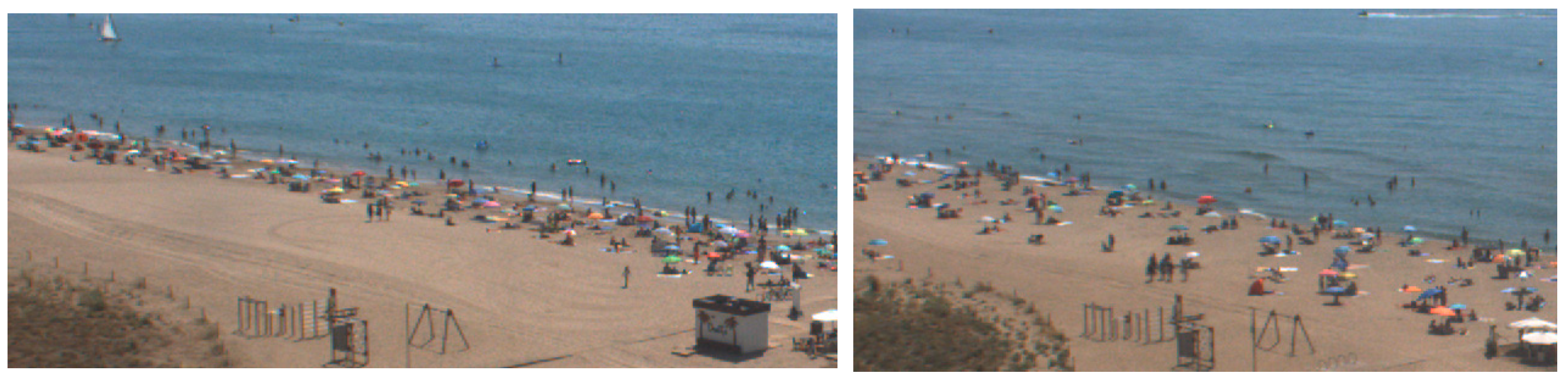
In terms of spatial distribution, changes are observed between pre-COVID-19 and pandemic years, as shown in Figure 8. An example of this change can be observed in the heat maps of two high attendance days, 9 August 2018 (left) and 19 August 2020 (pandemic year) (right), at 11:00 h. Before COVID-19, there was a higher concentration of people near the shore (non-uniform distribution). During COVID-19, pandemic beach users are located following a uniform distribution, trying to respect social distance recommendations.

4. Experiments and Results

Next, we present the experimental settings and the evaluation metrics and show the results.

4.1. Experimental Settings

The proposed deep learning algorithm was implemented in Python 3.7.3.

A neural network can learn something different from what its trainer had in mind [41]. A case of useless learning is when the neural network memorizes the training examples without learning what they have in common. A trained network is able to generalize when it can classify data from the same class as the learning data but that it has never seen before. This ability requires that the network is tested with an independent dataset. Therefore, the data samples were divided as follows: 70% of the samples were used for the training dataset (70% of 2498 records = 1748 records for the training phase) and 30% for the testing dataset (30% of 2498 records = 750 for the testing phase).

The input attributes were normalized. The proposed DNN consists of one input layer with 7 neurons that match the 7 input attributes, 6 hidden layers each with 300 neurons, and one output layer with one neuron for the modeling target.

Our proposed DNN was trained for the beach visitors classification task. In the dataset, the number of beach visitors was assigned to one of the 7 classes (or beach occupancy levels): 0–49, 50–99, 100–149, 150–199, 200–249, 250–299, and 300+. The class distribution is shown in

Table 1. Class distribution of beach visitors.

Classes (Beach Visitors)	Number of Samples	Percentage of Total Samples
0–49	272	15.56
50–99	685	39.19
100–149	372	21.28
150–199	280	16.02
200–249	17	0.97
250–299	91	5.20
300+	31	1.77

. The total number of records (1748) refers to the training phase.

Overfitting refers to a deep learning model that has a small loss function on the training data, and the prediction accuracy is high; however, on the test data, the loss function is relatively large and the prediction accuracy is low. To overcome the overfitting constraint, a grid search was conducted to find the best hyperparameters of the deep neural network using 10-fold cross validation. In a 10-fold cross validation scheme, the dataset is divided into 10 blocks of approximately equal size. In this case, 90% or 9 blocks of the data are used for training, and 10% or 1 block of the data is used for testing. This process is repeated 10 times, with a different data block used for testing each time.

Table 2. Class distribution of beach visitors.

Training-Testing Partition (%)	Total Training Records	Total Testing Records
70–30	1748	750
10-fold cross validation	2248	250

shows the number of training and testing instances in each partition scheme. The total number of records for the training (1748) and testing (750) phases is specified. The resulting values for the hyperparameters of the neural network training are presented in

Table 3. Hyperparameters.

Hyperparameter	Specification
Number of hidden layers	6
Number of neurons per hidden layer	300
Optimizer	Adam
Learning rate	0.001
Activation function	ReLU

. In order to solve the overfitting problem, we also introduced the dropout parameter (dropout value of 0.1), which achieved the regularization effect.

We evaluated the SGD, RMSprop, Adam, Adagrad, Adamax, and Nadam optimizers using the grid search technique. The Adaptive Moment Estimation (Adam) optimizer was selected to minimize the loss function and speed up the training process because it obtains the best results.

The Adam optimizer is one of the most popular gradient descent optimization algorithms since it is computationally efficient and has very little memory requirement. This method calculates the individual adaptive learning rate for each parameter from estimates of first and second moments of the gradients.

The Adam algorithm (see Algorithm 1) first updates the exponential moving averages of the gradient ($m_t$) and the squared gradient ($v_t$), which is the estimate of the first and second moment. The hyperparameters ${\beta }_1$, ${\beta }_2$∈ [0, 1) control the exponential decay rates of these moving averages, as shown in the following equations:

$$m_t={\beta }_1{m}_{t-1}+\left(1-{\beta }_1\right)g_t$$

(3)

$$v_t={\beta }_2{v}_{t-1}+\left(1-{\beta }_2\right)g_t^2$$

(4)

where $g$ is the current gradient value of error function for the neural network training.

Algorithm 1 Adam, our proposed algorithm for the training process.

1: Declare the parameters Objective function $f\left(\theta \right)$, hyperparameter learning rate $\alpha$, exponential decay rates ${\beta }_1$, ${\beta }_2$ for moment estimates, tolerance parameter $ϵ>0$ for numerical stability 2:  Initialize first moment vector $m_0=0$, second moment vector $v_0=0$ and timestep $t=0$ 3:  while ${\theta }_t$ has not converged do 3.1 update timestep $t=t+1$ 3.2 compute gradient of objective using $g_t={▽}_{\theta }{f}_t\left({\theta }_t-1\right)$ 3.3 update first moment estimate and second moment estimate using Equations (3) and (4), respectively. 3.4 compute unbiased first and second moment estimate using Equations (5) and (6), respectively. 3.5 update objective parameters using Equation (7). end while 4: return final parameter ${\theta }_t$

Moving averages are initialized as 0. The moment estimates are biased around 0, especially during the initial timesteps. This initialization bias can be easily counteracted resulting in bias-corrected estimate.

$${\widehat{m}}_t=\frac{m_t}{1-{\beta }_1^t}$$

(5)

$${\widehat{v}}_t=\frac{v_t}{1-{\beta }_2^t}$$

(6)

Finally, we update the parameter ${\theta }_t$ as shown below:

$${\theta }_t={\theta }_{t-1}-\frac{\alpha {\widehat{m}}_t}{\sqrt{{\widehat{v}}_t}+\epsilon }$$

(7)

We used in our experiments for the Adam optimizer a learning rate $\alpha ={10}^{-3}$ and two decay parameters ${\beta }_1$= 0.9 and ${\beta }_2$= 0.999 [42].

Experiments were carried out on a laptop running 64-bit Windows 10 Home on an Intel Core i5-8265U and using 8 GB of memory.

4.2. Evaluation Metrics

Five different metrics were used to evaluate the performance of the proposed scheme: Mean Absolute Error (MAE), accuracy, precision, recall, and F1-score. F1-score is the harmonic mean of precision and recall.

The selected metrics can be calculated as follows:

$$Accuracy=\frac{TP+TN}{TP+TN+FP+FN}$$

(8)

where TP represents true positives, TN represents true negatives, FP represents false positives, and FN represents false negatives.

$$MAE=\frac{1}{K}{\displaystyle \sum }_{k=1}^K\left|g_k-g{\prime }_k\right|$$

(9)

where $g_k$ and $g{\prime }_k$ represent the real and predicted number of beach visitors, respectively, and K denotes the total number of testing samples.

$$Precision=\frac{TP}{TP+FP}$$

(10)

$$Recall=\frac{TP}{TP+FN}$$

(11)

$$\mathrm{F}1-\mathrm{score}=\frac{2\times Precision\times Recall}{Precision+Recall}$$

(12)

4.3. Performance Evaluation

Figure 9 and Figure 10 illustrate the loss function convergence curve and accuracy curve of the neural network training and testing phases for beach occupancy prediction, respectively. The decreasing loss and the increasing accuracy curves in Figure 9 and Figure 10, respectively, generally suggest that the neural network model is learning to generalize on the target problem.

To figure out the performance of the developed DNN, Figure 11 shows the confusion matrices on the test set (1) only for June, (2) only for July, (3) only for August, and (4) for the whole dataset (June, July, and August). The classification error for June (see Figure 11a) came mainly from the prediction of classes 150–199, 200–249, 250–299, and 300+. The reason is that there are fewer training samples for these classes, since the prime bathing season starts in June, and during this month, fewer people come to the beach. In July (Figure 11b) and August (Figure 11c), beach visitors of all classes are well predicted, with the exception of class 200–249 for July, since there are very few training samples for this class. No sample of class 300+ can be predicted for August, because during this month, the residents in Spain have holidays; they tend to travel far away from the cities, and Castelldefels beach is located very close to the city of Barcelona. All classes are well predicted for the whole dataset (Figure 11d).

The accuracy, precision, recall, and F1-score for all the classes and the whole data set were computed using the confusion matrix. The results as well as the number of instances per class for the test set are shown in

Table 4. Comparison of accuracy and F1-score for all classes.

Classes (Beach Visitors)	Accuracy	Precision	Recall	F1-Score	Number of Samples per Class for the Test Set
0–49	0.99	0.98	0.99	0.99	121
50–99	0.94	0.94	0.90	0.92	302
100–149	0.96	0.88	0.92	0.90	159
150–199	0.98	0.93	0.93	0.93	110
200–249	1	1	0.90	0.95	10
250–299	0.99	0.83	0.97	0.90	36
300+	1	0.92	1	0.96	12

. Accuracy is not a very good measure of performance when dealing with unbalanced datasets (like our case) because it counts the number of correct predictions regardless of the type of class. For this reason, it is biased towards the majority classes.

As we can see in Table 4, the accuracy is extremely high (0.99 or 1), even when the model fails to identify some samples of minority classes (such as classes 200–249, 250–299, and 300+). Since accuracy gives biased results with unbalanced data, it is not a good metric to use. Therefore, we selected precision and recall, together with F1-score, as more reliable measures.

Table 5. MAE, accuracy, precision, recall, and F1-score.

Dataset Size	MAE	Accuracy	Precision	Recall	F1-Score
June	0.0553	0.84298	0.844526	0.836719	0.837623
July	0.03069	0.94219	0.935523	0.935185	0.934539
August	0.04055	0.94801	0.946325	0.944	0.943866
whole dataset	0.03059	0.9269333	0.929422	0.926933	0.927114

reports the results of our analysis for every category in the test set using the MAE, accuracy, precision, recall, and F1-score. The results of 10 independent runs are shown. We present the results (1) only for June, (2) only for July, (3) only for August, and (4) for the whole dataset.

The DNN achieves the highest F1-score, with a value of 94.3866%, for August and a high F1-score of 92.7114% for the whole data set. The lowest results in terms of F1-score are obtained when the DNN is trained just for June, since the video cameras were unavailable during several days, and these days were essential to train the DNN. This fact suggests that training with more images would improve the classification. Furthermore, from the confusion matrixes, it can be observed that in June (when the beach attendance is lower) there are fewer samples to train categories with a high number of beach visitors, and this causes the DNN to fail in the prediction. Nevertheless, the F1-scores for all months maintain a high level, which proves the feasibility of the DNN. Precision and recall have similar values. A higher F1-score is caused by higher precision and recall values, and vice versa. The accuracy values are also high and similar to the F1-score values. Finally, we notice that for the whole dataset, the best MAE of 0.03059 is obtained.

Table 6. Per-class precision, recall, and F1-scores for the time period 2016–2018.

Classes (Beach Visitors)	Precision	Recall	F1-Score
0–49	0.981	0.981	0.982
50–99	0.943	0.898	0.919
100–149	0.865	0.925	0.892
150–199	0.92	0.956	0.9323
200–249	0.925	0.849	0.879
250–299	0.939	0.914	0.926
300+	0.93	0.97	0.949

presents the evaluation of the DNN in every category using the precision, recall, and F1-scores for 10 independent runs. The DNN performs well in the classification task for all categories.

The best per-class F1-scores are obtained for different types of categories: a very reduced number of beach visitors (0–49), a very high number (300+), and a medium number (150–199). The categories 50–99 and 200–249 show the worst results for the F1-score due to the increase of false negatives (recall). The category 100–149 has an F1-score of 89.2% due to the increase of the false positives (precision). Nevertheless, the precision rate, recall, and F1-score are relatively stable for all categories.

The performance of the proposed DNN for the whole dataset was investigated with different batch sizes. The results of 10 independent runs are shown in

Table 7. F1-score for different batch sizes.

Batch Size	F1-Score
16	0.88511
32	0.917197
64	0.923412
128	0.917907
256	0.91545

. With a batch size of 64, the best F1-score of 92.3412% is achieved.

In order to check the robustness of the results, the model was revaluated for the time periods 2018–2020 and 2019–2021.

Table 8. Per-class precision, recall, and F1-scores for the time period 2018–2020.

Classes (Beach Visitors)	Precision	Recall	F1-Score
0–49	0.891	0.927	0.91
50–99	0.935	0.912	0.923
100–149	0.931	0.856	0.892
150–199	0.941	0.905	0.922
200–249	0.893	0.903	0.90
250–299	0.931	0.981	0.955
300+	0.945	0.927	0.936

and

Table 9. Per-class precision, recall, and F1-scores for the time period 2019–2021.

Classes(Beach Visitors)	Precision	Recall	F1-Score
0–49	0.931	0.917	0.924
50–99	0.915	0.931	0.923
100–149	0.951	0.888	0.918
150–199	0.932	0.861	0.895
200–249	0.934	0.94	0.937
250–299	0.893	0.963	0.927
300+	0.951	0.936	0.943

present the evaluation of the DNN in every category using the precision, recall, and F1-scores for the selected time periods and 10 independent runs. The DNN performs well in the classification task for all categories. In the time period 2018–2020, the best per-class F1-scores are obtained for different types of categories: a reduced number of beach visitors (50–99) and a high/very high number (250–299)/(300+). The category 100–149 shows the worst results for the F1-score due to the increase of false negatives (recall). The category 200–249 has an F1-score of 90% due to the increase of the false positives (precision). In the time period 2019–2021, the best per-class F1-scores are obtained for categories with a high/very high number of beach visitors (200–249; 250–299)/(300+). The categories 100–149 and 150–199 show the worst results for the F1-score due to the increase of false negatives (recall). We observe that for both time periods, the precision rate, recall, and F1-score are relatively stable for all categories. Therefore, we can conclude that the robustness of the model is not affected by the time periods chosen.

4.4. Network Depth

The DNN topology was also investigated in detail to improve the modelling performance.

Two critical DNN topology parameters are the network depth (number of hidden layers) and width (number of neurons per hidden layer) [43]. We tested different DNN topologies, where the number of hidden layers varies between 1 and 6 and the number of neurons per hidden layer varies between 30 and 300.

The performance impact of the network depth is shown in Figure 12. The MAE of 10 independent runs is shown. The number of neurons per hidden layer is 300, and the number of layers varies between 1 and 6. It can be observed that when the number of hidden layers is increased, the modeling performance of the deep neural network is improved. The median MAE for the number of beach visitors improves from 0.04655 with one hidden layer to 0.03045 for six hidden layers, with a 34.6% improvement. However, the improvement slows down when more layers are added. The improvement becomes insignificant with more than four hidden layers. The median MAE for the number of beach visitors shows a 34.2% decrease from 0.04655 with one hidden layer to 0.03065 with four hidden layers; however, when the number of hidden layers is increased to six, only a 0.65% decreased is achieved, with 0.00036 modeling accuracy variation. We observe that the deep neural network can maintain a good modelling performance when the number of layers is increased and does not suffer overfitting. We conclude that the model is not biased with the training data and keeps improving when the number of neurons raises.

4.5. Network Width

Next, we study the impact of network width, or the number of neurons per hidden layer. The performance impact of the network width is shown in Figure 13. The results are shown with six hidden layers, and the width varies between 25 and 300. We see that the modeling performance is better when the number of neurons is increased. It can also be observed that the modeling performance after 175 neurons per hidden layer improves very slowly when more neurons are added. However, the convergence speed in network width is faster than that of network depth. Doubling one hidden layer to two layers decreases the median MAE from 0.04655 to 0.03485, by 25.13%, and further doubling to four layers improves the MAE to 0.03045, by 12.62%.

Regarding the network width, doubling the number of neurons per layer from 25 neurons to 50 reduces the MAE from 0.08045 to 0.05025, by 37.54%, and further doubling to 100 neurons achieves a 0.0372 median MAE, with 25.97% improvement. These results reflect the fact that an increase in the number of hidden layers and the number of neurons per hidden layer has a different impact on the deep neural network. In a fully connected neural network, every neuron in each layer of the network is connected to every other neuron in the adjacent forward layer. If such a neural network has n neurons per layer and m hidden layers, the total number of neuron links is $O\left(m{n}^2\right)$. Since the number of neuron links scales linearly with network depth but exponentially with network width [43], the network performance improves more significantly as the network widens.

4.6. Optimal Network Topology

Next, we study the optimal network topology. We consider five different network topologies that maintain the total number of neurons (1800). The first topology, denoted as FIRST, consists of a neural network with six hidden layers and 300 neurons evenly distributed in each layer. The second topology (SECOND) considers fewer hidden layers, with more neurons per layer than the FIRST case. Specifically, the neural network consists of three hidden layers, with 600 neurons per layer. The third topology (THIRD) considers more hidden layers, with fewer neurons per layer than the FIRST case. It consists of 12 layers, with 150 neurons per layer. The fourth topology (FOURTH) assumes there is an increase in the number of neurons for deeper hidden layers. The number of neurons is increased for each hidden layer as follows: 200 (for the first hidden layer), 200, 300, 300, 400, and 400 (for the last hidden layer). The last topology (FIFTH) assumes there is a decrease in the number of neurons for deeper hidden layers (the reverse order of the proposed FOURTH topology). The modelling performance using the five topologies is shown in Figure 14. The fifth topology (FIFTH) achieves the best overall performance, with a median MAE of 0.02735, which is 9.59, 12.34, 23.82 and 1.26% more accurate than the models FIRST, SECOND, THIRD and FIFTH, respectively. The FOURTH and FIFTH topologies achieve a better modeling performance. Therefore, we conclude that a fatter and especially a thinner topology improves the modeling performance.

4.7. Comparison to Other Models

Python libraries enable the deployment of many traditional models. Scikit-learn is an open-source machine learning library that supports supervised and unsupervised learning. It offers several tools for model fitting, data preprocessing, model selection and evaluation, and many other utilities.

We compared our proposal with three well-known models provided by the scikit-learn library, which support multiclass classification. These classifiers are decision tree, k-nearest neighbor (kNN), and random forest.

We also employed 10-fold cross validation for the evaluation and comparison of these machine learning algorithms.

Table 10. Per-class precision, recall, and F1-scores. Comparison between our proposed DNN and other traditional machine learning models.

	Accuracy	Precision	Recall	F1-Score
Our DNN	0.927	0.929	0.927	0.927
Decision tree	0.892	0.87	0.88	0.875
K-nearest neighbor	0.593	0.65	0.68	0.664
Random forest	0.412	0.61	0.56	0.584

shows the results achieved by our deep neural network model and these traditional models.

The analysis shows that our proposed DNN model achieves the highest accuracy, precision, recall, and F1-score of 92.7%, 92.9%, 92.7%, and 92.7%, respectively, compared to traditional machine learning models. We also observe that, of the traditional models, decision tree achieves the highest accuracy, precision, recall, and F1-score of 89.2%, 87%, 88%, and 87.5%, respectively, followed by k-nearest neighbor, with an accuracy, precision, recall, and F1-score of 59.3%, 65%, 68%, and 66.4%, respectively. We can conclude that our proposed algorithm outperforms other traditional machine learning algorithms and is able to perform beach attendance predictions adequately.

5. Discussion

Several authors [18,19,20,21,22,24] have analyzed how beach attendance is affected by weather conditions and other aspects such as time, season, etc. The results indicate that beach attendance is affected by the season, day, hour, and meteorological conditions. Our results confirm the same trend.

Our results regarding the daily temporal distribution of beachgoers are consistent with other beaches along the Mediterranean Sea [18,19,20].

Other authors have used classical econometric models to simulate the seasonality and cyclicality of the processes. In [18], the authors modelled the number of beachgoers as a function of temperature, for temperatures lower than 30 °C, using the regression coefficient R² = 0.87 at the Lido of Sète Beach, France. In [21], regression methods are used to determine how the number of beachgoers is affected by the season, day, weather, and ocean conditions (maximum significant wave height, water temperature) in Australian beaches. The authors use ordinal logistic regression to distinguish between three categories of beach visitor numbers: high, moderate, and low. The authors in [19] sought a mathematical expression to model beach attendance. The observed mean number of daily users was adjusted to a time-dependent Fourier polynomial for two beaches in Barcelona. The occupation data for 2002–2004 were averaged to obtain an estimation of the occupation trend for a typical year. This averaged function was projected into a 14-term Fourier polynomial. The Fourier fit obtained and the original time series of the average occupation in a typical year adjusted 74% and 69% of the absolute value of the original time series for the two beaches, respectively. In contrast, our proposed DNN improves these results. It can predict well the number of beach visitors assigned to any of the seven classes or beach occupancy levels and obtains a good performance, with an accuracy of 92.7%.

6. Conclusions

In this paper, experimental research that uses IoT data and deep learning to estimate beach attendance at Castelldefels beach (Barcelona, Spain) was developed, and beach attendance was predicted. Images of Castelldefels beach were captured by a video monitoring system.

An image recognition software was used to estimate the number of beachgoers per hour from 9:00 to 19:00 h during June, July, and August (prime swimming season) from 2016 to 2018. It was verified that the automated count was not significantly different from the manual count, and thus this methodology is suitable for the evaluation of beach attendance. The detection algorithm was not able to estimate the number of beachgoers with cloudy, rainy weather or blurry images. To solve this problem, the number of beach visitors was counted manually. However, the detection algorithm saved time and provided good results for a huge number of images. It would also be necessary to perform additional training of the detection algorithm to improve its accuracy in distinguishing special cases: beach goers riding their bicycles, beach goers covered partially by umbrellas at the beach, etc.

It was shown that weather, time, season, and working day/holiday have significant effects on the number of beachgoers. More resources (e.g., lifeguards, police officers that patrol the beaches, etc.) will be required during weekends or public holidays to protect beach visitors, especially during prime seasons.

Furthermore, a deep learning algorithm was trained for the first time for beach attendance prediction. The experimental results prove the feasibility of DNNs for beach attendance prediction. The confusion matrices on the test set were shown for June, July, and August. All classes are well predicted for the whole dataset. In our testing experiments, the proposed DNN yields a very good performance with an MAE, accuracy, precision, recall, and F1-score of 0.03, 92.7%, 92.9%, 92.7%, and 92.7%, respectively. Our proposed deep learning classifier outperforms other machine learning models (decision tree, k-nearest neighbor, and random forest) and can successfully differentiate between seven beach occupancy levels. The best F1-scores are obtained for a very reduced number of beach visitors (0–49), a very high number (300+), and a medium number (150–199), with values of 98.2%, 93.23%, and 94.9%, respectively. The impact of the DNN topology was also investigated. The results show that the DNN performance improves when the number of hidden layers is increased. It also improves with more neurons per hidden layer. The modeling accuracy benefits from an increase in the number of neurons for deeper hidden layers (fourth topology), and the best results are obtained when there is a decrease in the number of neurons for deeper hidden layers (fifth topology).

This research has two limitations. First, only one beach in Castelldefels is considered. This research could be extended to other beaches in Castelldefels. Second, the weather data are taken from a weather station of Meteocat (Meteorological Service of Catalonia) that is located in Viladecans, near but not at the respective beach. However, we expect that these registered weather conditions are reasonably accurate for our case study.

This work has shown that coastal videometry and image processing are very efficient tools for beach attendance detection. Furthermore, beach attendance prediction was successfully developed, and it is of particular importance for coastal managers to plan beach services in terms of security, rescue, health, and environmental assistance.