
An Intelligent Clustering-Based Routing Protocol (CRP-GR) for 5G-Based Smart Healthcare Using Game Theory and Reinforcement Learning


Abstract
:1. Introduction
Our Contribution
- Clustering-based routing protocol using game theory and reinforcement learning to reduce energy consumption and increase network lifetime for smart healthcare scenarios.
- An algorithm to select the best optimal cluster head (CH) from the available cluster heads (CHs) to avoid the situation of more cluster head (CH) occurrence.
- Reinforcement learning-based route selection algorithm for data transmission.
- Comparison of existing approaches with the proposed method.
2. Literature Review
3. System Model
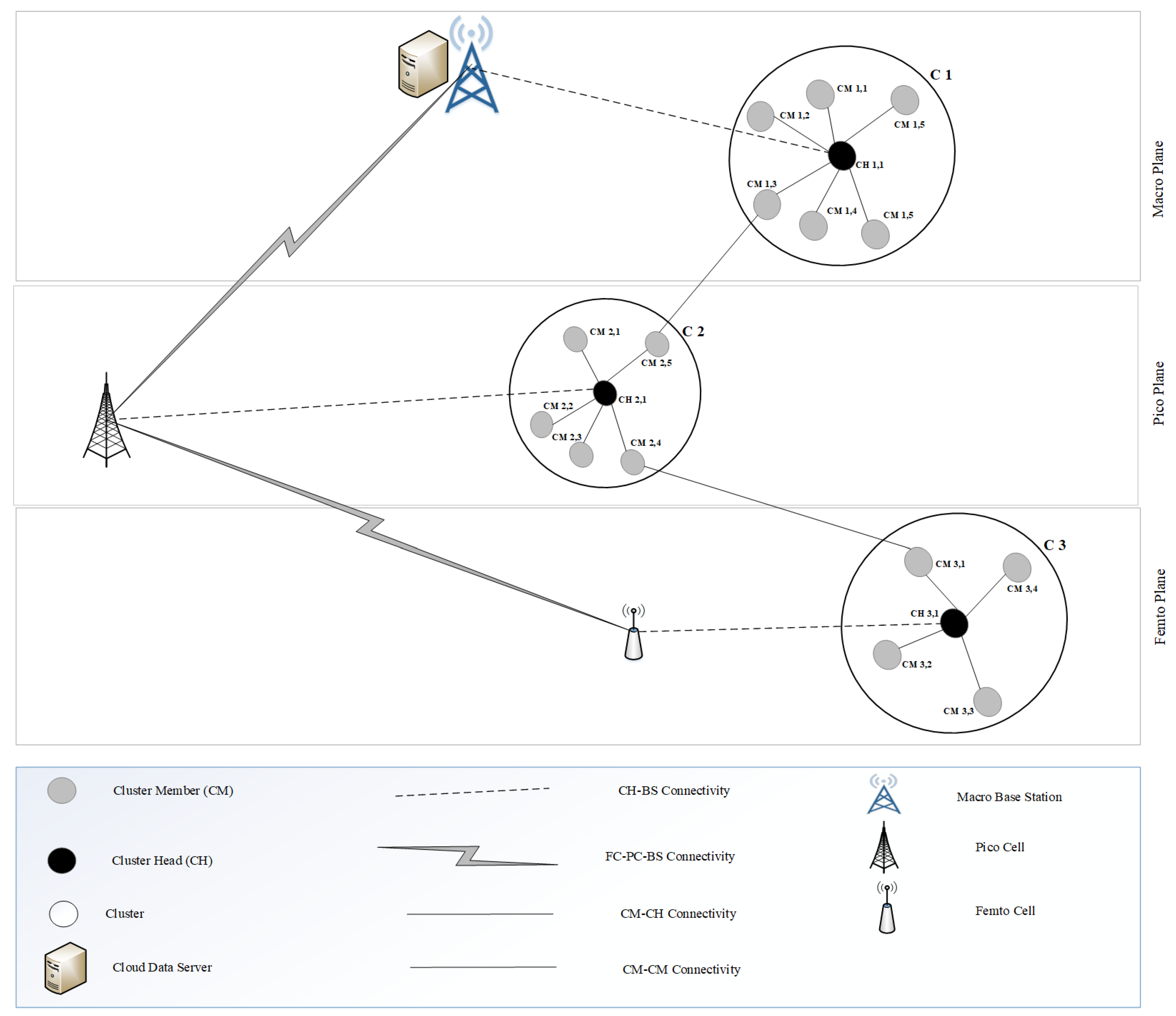
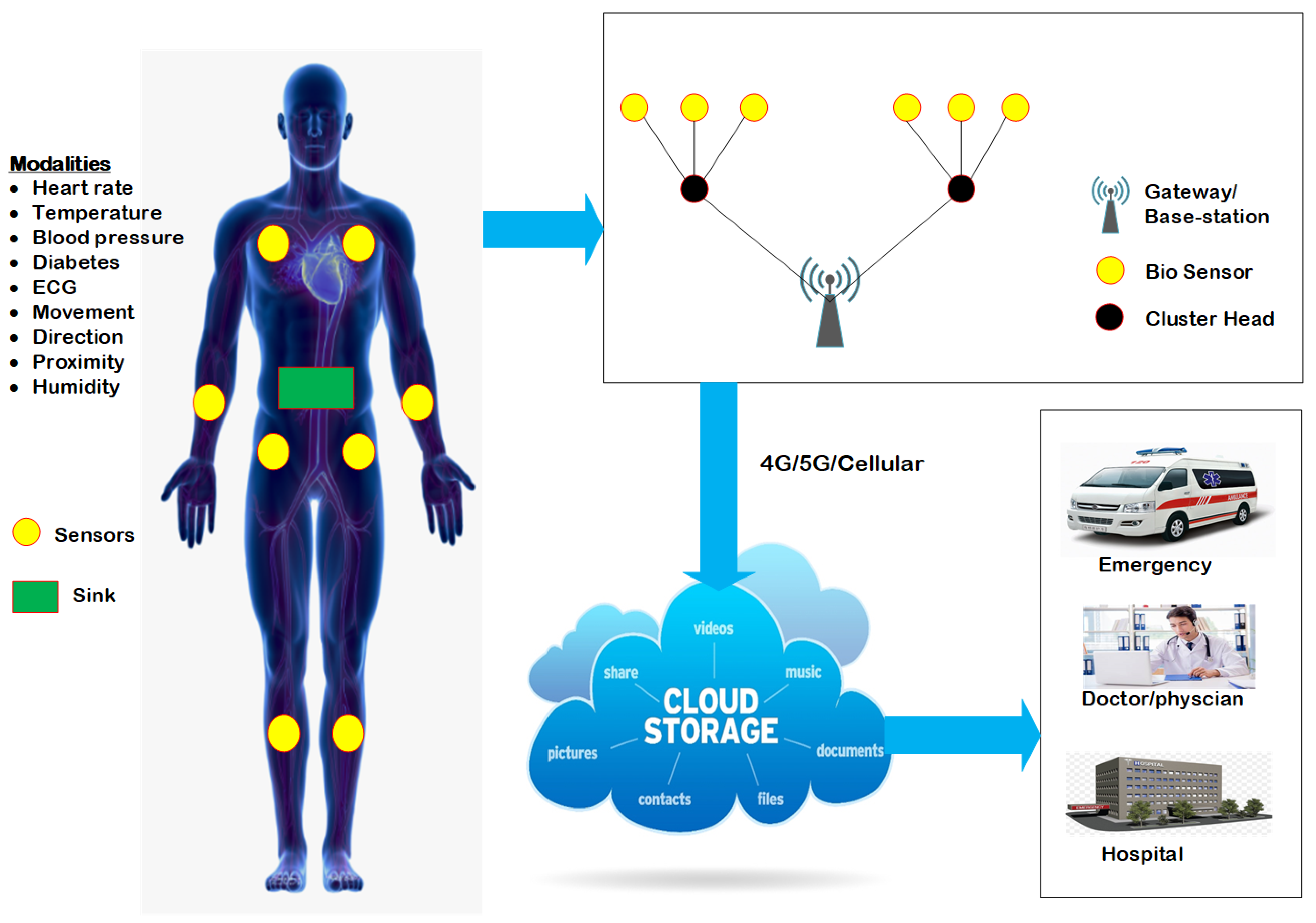
3.1. Network Model
- All the sensors nodes in the network are mobile after the deployment.
- All three different categories of nodes have different energy levels. We consider picocells as advanced cells, femtocells as intermediate nodes, and other nodes as normal.
- All sensor nodes in the network have different mobility speeds and energy levels.
- The battery in each node in the network has a different initial energy level, and it is not rechargeable or replaceable.
- All sensor nodes in the network have their unique ID.
3.2. Energy Model
3.3. Cluster Game Modelling
- Player: N number of nodes
- Action: Cluster head (CH) and non-cluster head (NCH) are sets of actions for each player.
- Utility: Utilities of each player are denoted by the expected payoff function value, which is “0” which means no node declares as cluster head (CH).
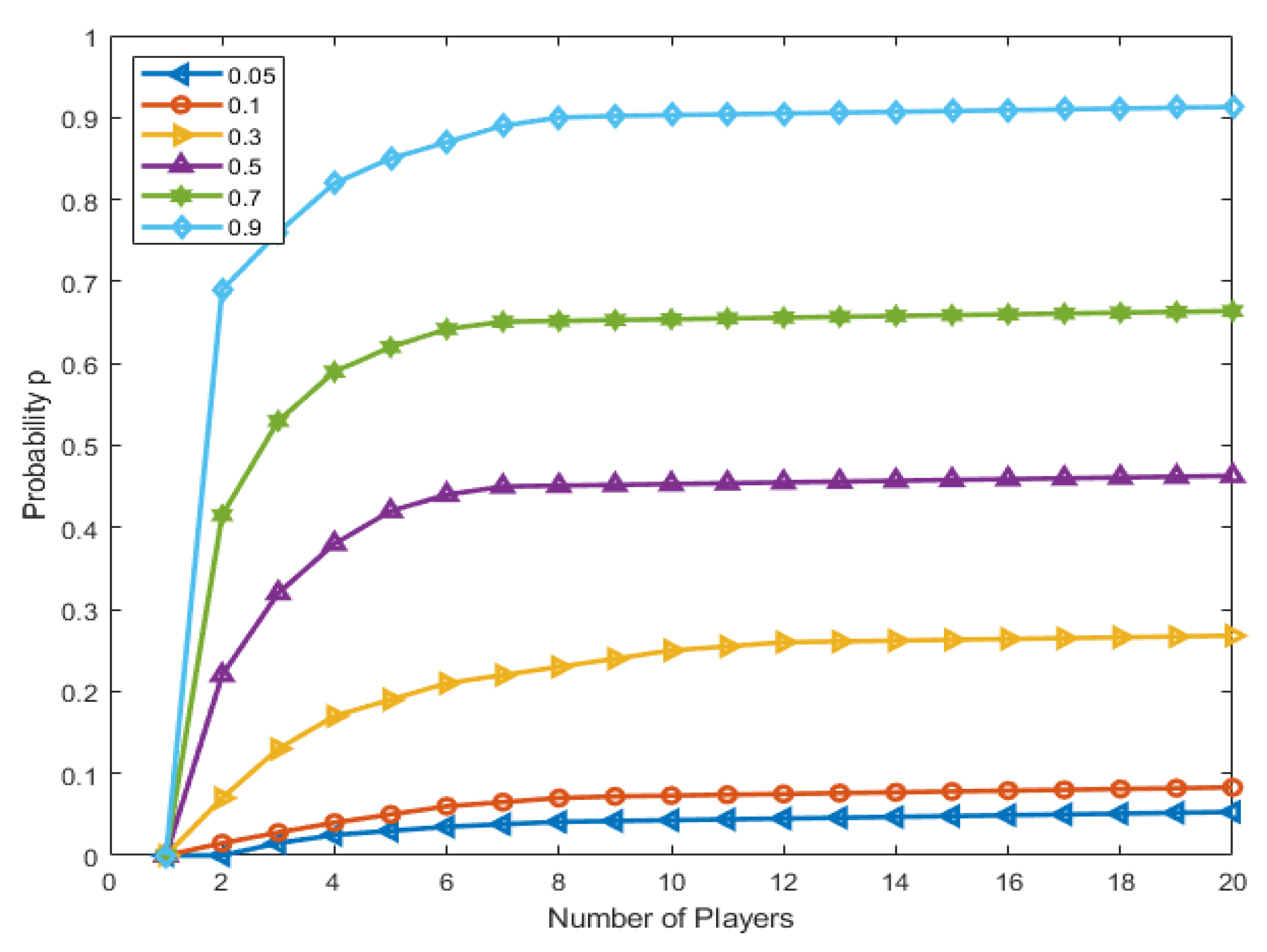
3.4. Expected Payoff
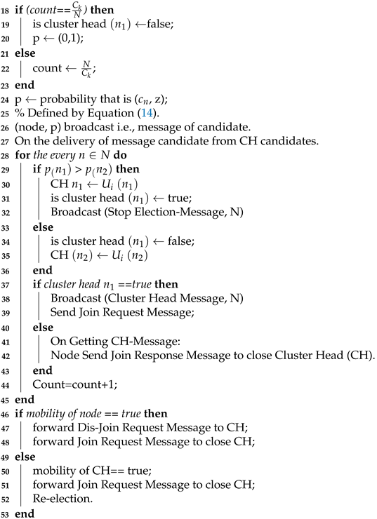
4. Clustering Algorithm
4.1. Initialization
4.2. Setup Phase
4.3. Steady-State Phase
| Algorithm 1: Clustering |
| 1 Require: N: Number of nodes. |
| 2 : Nodes among N. |
| 3 : Node utility function. |
| 4 : node probability to become a cluster head (CH). |
| 5 : Total number of times as to be a cluster head (CH). |
| 6 : Number of optimal clusters. |
| 7 Ensure: CH(): Cluster Head selection of the node . |
| 8 Functions: |
| 9 Broadcast (Distance, Data); |
| 10 Send (Data, Destinations); |
| 11 Probability (, z); |
| 12 % Initialization |
| 13 ← n(CH, NCH). |
| 14 is cluster head = false; |
| 15 r ← 0. |
| 16 MAIN: |
| 17 For each round of clustering. |
 |
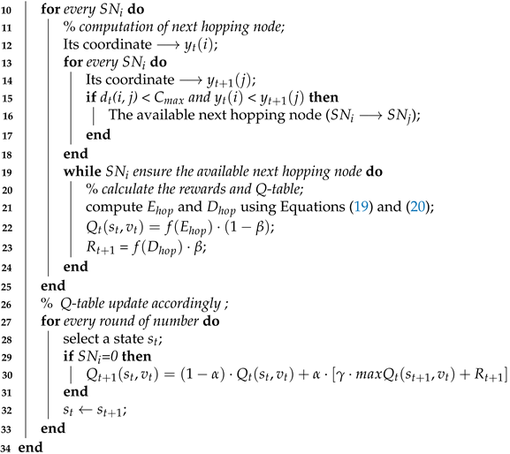
5. Routing Algorithm
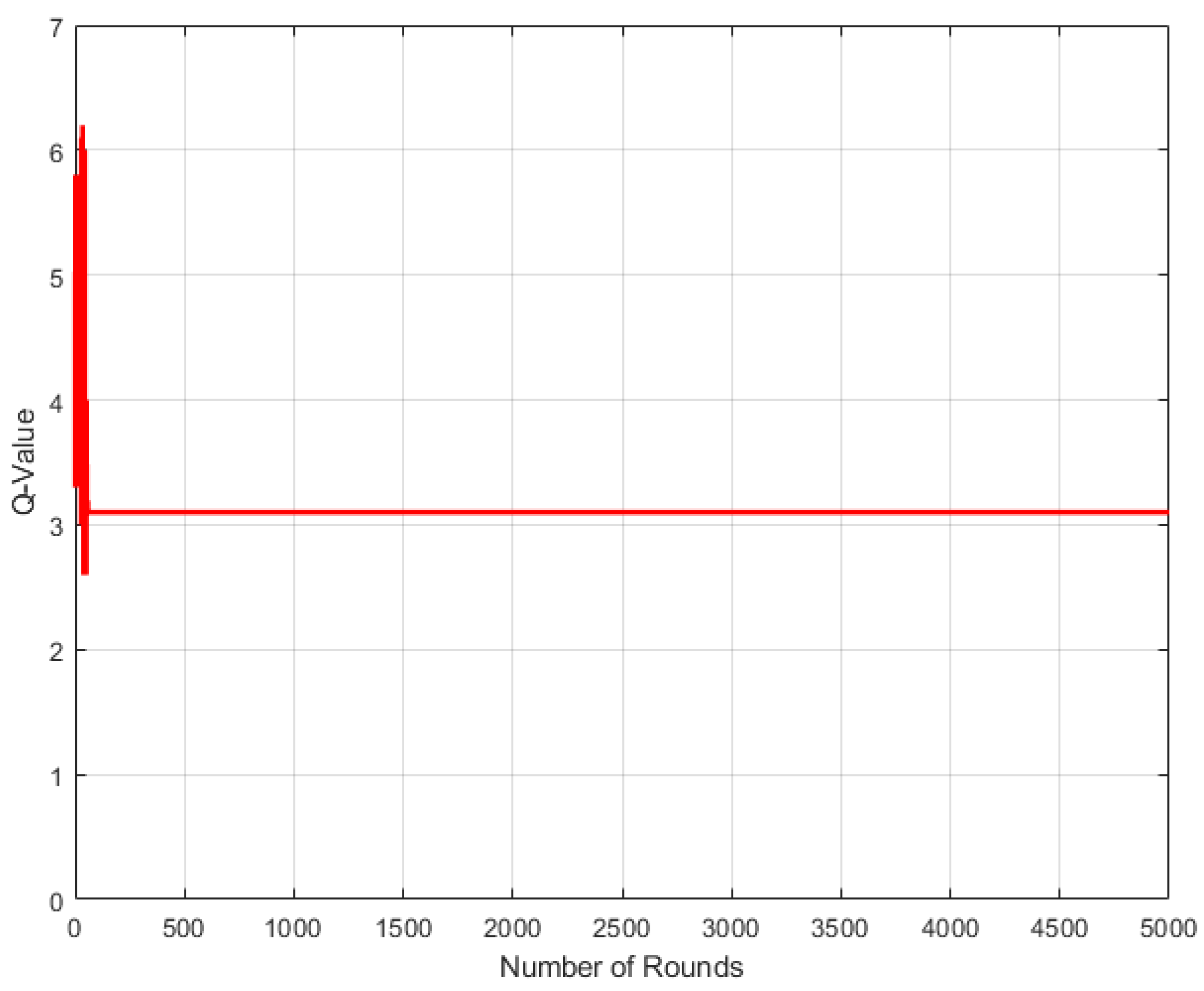
5.1. Q-Learning
5.2. Our Proposed Routing Algorithm
| Algorithm 2: QL-Algorithm |
| 1 Require: Information of nodes |
| 2 Ensure: Q-table |
| 3 % Initialization; |
| 4 Zeros-matrix ⟶ Q-table; |
| 5 Distance between nodes ⟶ ; |
| 6 Maximum communication distance ⟶ ; |
| 7 Energy remaining of nodes ⟶ ; |
| 8 % Run clustering algorithm; |
| 9 while CHs sets are not empty do; |
 |
| Algorithm 3: Best Path Selection Scheme |
| 1 Require: Information of node |
| 2 Ensure: Best path selection |
| 3 % Initialization |
| 4 All nodes update BS about their location and remaining energy. |
| 5 On the basis of algorithm 1 Base station form clusters in the network and calculate the Q-table. |
| 6 % Data Sending |
| 7 for every source node do |
 |
6. Time Complexity of Proposed Algorithms
6.1. Time Complexity Clustering Algorithm
- Use the if-else statement from lines 18–23 to check count = and count ←, taking a constant time due independent of data length. We denote this constant with .
- p ← (, z) taking a constant time and denoting with . It executes once by receiving a pre-calculated value.
- The statement if-else from lines 28–43 repeats for N number of nodes. This means that the probability p() will repeat n times and probability p() will also repeat n times. The time taken will be times.
- Count = count + 1 will take n times to execute.
- The if-else statement from lines 46–53 takes a constant time to execute. We denote it as and .
6.2. Time Complexity of the Q-Learning Algorithm
- The for-loop statement from lines 10–13 takes n seconds to compute the next hopping node, and lines 14–20 take n seconds to check for available next hopping nodes. Therefore, it will take times due to the inner loop.
- For calculating the reward and Q-table, the while-loop form lines 21–27 takes n time.
- For updating the Q-table, the for-loop form lines 29–33 takes n time.
- Changing state ← takes a constant time.
6.3. Time Complexity of the Best Path Selection Algorithm
- The for-loop from lines 7–9 will take n time.
- The while-loop from lines 10–16 will take n time.
- DThe inner loop form lines 7–21 is takes times.
7. Results and Discussion
7.1. Evaluation Metrics
7.1.1. Throughput
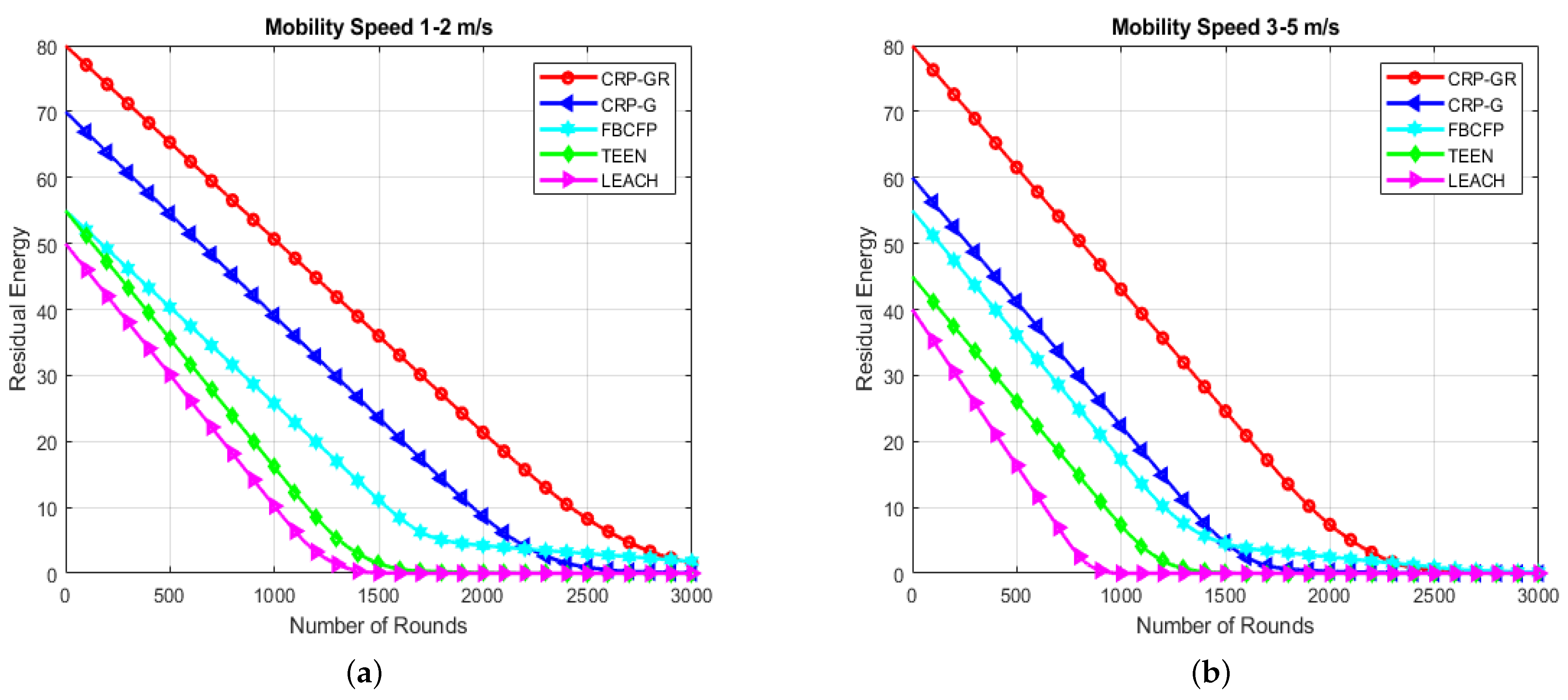
7.1.2. Residual Energy
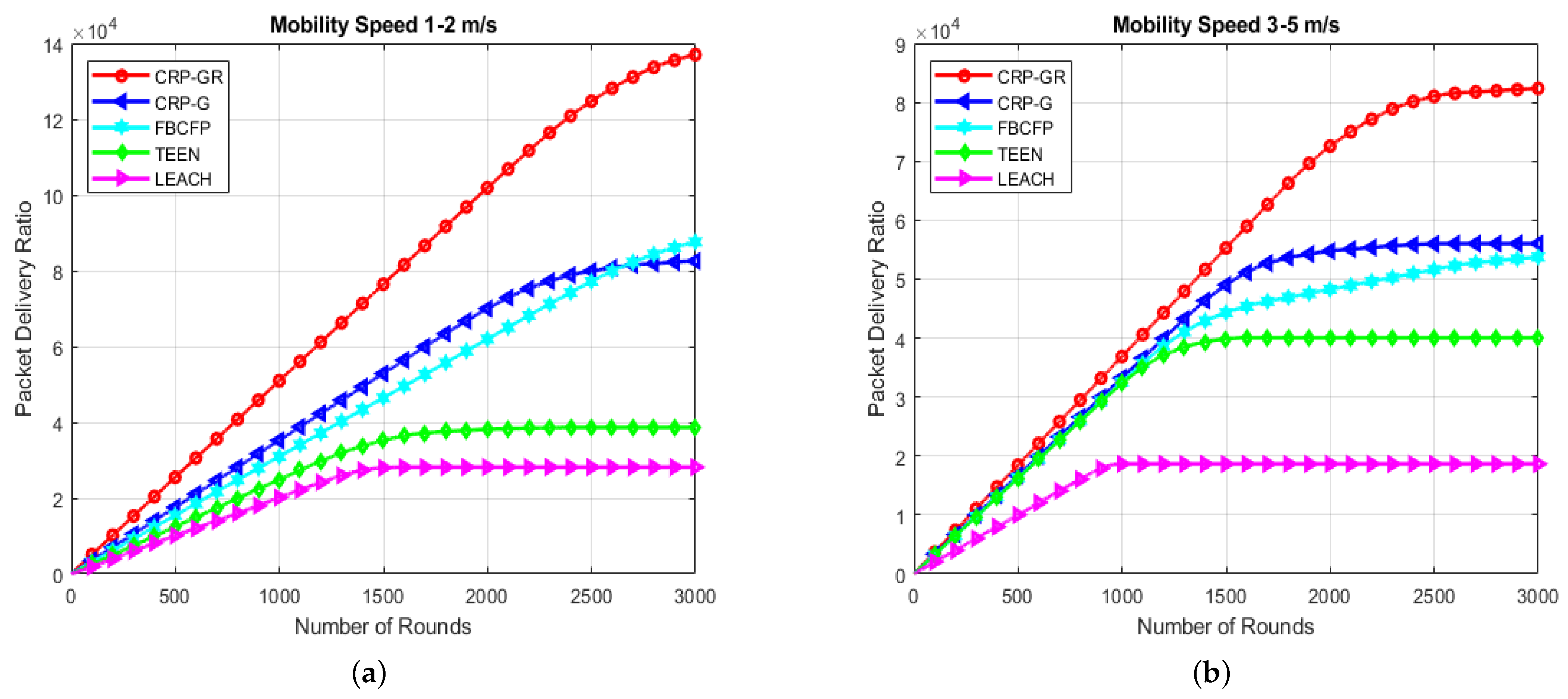
7.1.3. Packet Delivery Ratio
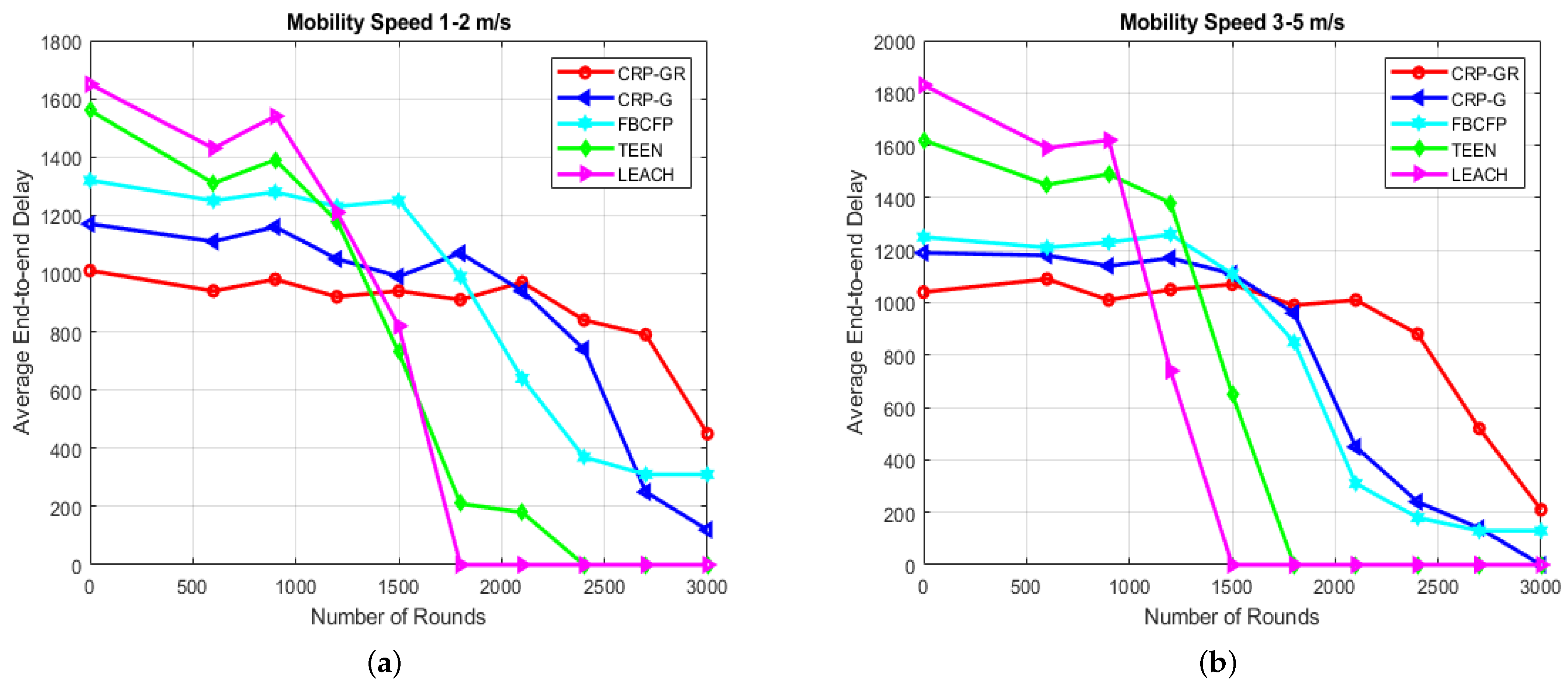
7.1.4. Average End-to-End Delay
7.1.5. Network Lifetime
7.2. Results
7.2.1. Throughput
7.2.2. Packet Delivery Ratio
7.2.3. Residual Energy
7.2.4. Average End-to-End Delay
7.2.5. Network Lifetime
7.3. Discussion
8. Conclusions
Author Contributions
Funding
Institutional Review Board Statement
Informed Consent Statement
Data Availability Statement
Conflicts of Interest
References
- Pirbhulal, S.; Zhang, H.; Alahi, E.; Eshrat, M.; Ghayvat, H.; Mukhopadhyay, S.C.; Zhang, Y.-T.; Wu, W. A novel secure IoT-based smart home automation system using a wireless sensor network. Sensors 2017, 17, 69. [Google Scholar] [CrossRef] [PubMed]
- Ahad, A.; Tahir, M.; Alvin Yau, K.-L. 5G-Based Smart Healthcare Network: Architecture, Taxonomy, Challenges and Future Research Directions. IEEE Access 2019, 7, 100747–100762. [Google Scholar] [CrossRef]
- Kristoffersson, A.; Lindén, M. A Systematic Review on the Use of Wearable Body Sensors for Health Monitoring: A Qualitative Synthesis. Sensors 2020, 20, 1502. [Google Scholar] [CrossRef] [PubMed] [Green Version]
- Wu, W.; Pirbhulal, S.; Sangaiah, A.K.; Mukhopadhyay, S.C.; Li, G. Optimization of signal quality over comfortability of textile electrodes for ECG monitoring in fog computing based medical applications. Future Gener. Comput. Syst. 2018, 86, 515–526. [Google Scholar] [CrossRef]
- Pirbhulal, S.; Zhang, H.; Wu, W.; Mukhopadhyay, S.C.; Zhang, Y.-T. Heart-beats based biometric random binary sequences generation to secure wireless body sensor networks. IEEE Trans. Biomed. Eng. 2018, 65, 2751–2759. [Google Scholar] [CrossRef]
- Magsi, H.; Sodhro, A.H.; Chachar, F.A.; Abro, S.A.K.; Sodhro, G.H.; Pirbhulal, S. Evolution of 5G in Internet of medical things. In Proceedings of the 2018 International Conference on Computing, Mathematics and Engineering Technologies (iCoMET), Sukkur, Pakistan, 3–4 March 2018; pp. 1–7. [Google Scholar]
- Ahad, A.; Faisal, S.A.; Ali, F.; Jan, B.; Ullah, N. Design and performance analysis of DSS (dual sink based scheme) protocol for WBASNs. Adv. Remote. Sens. 2017, 6, 245. [Google Scholar] [CrossRef] [Green Version]
- Wu, W.; Pirbhulal, S.; Zhang, H.; Mukhopadhyay, S.C. Quantitative assessment for self-tracking of acute stress based on triangulation principle in a wearable sensor system. IEEE J. Biomed. Health Inform. 2018, 23, 703–713. [Google Scholar] [CrossRef]
- Farahani, B.; Firouzi, F.; Chang, V.; Badaroglu, M.; Constant, N.; Mankodiya, K. To- wards fog-driven IoT eHealth: Promises and challenges of IoT in medicine and health-care. Future Gener. Comput. Syst. 2018, 78, 659–676. [Google Scholar] [CrossRef] [Green Version]
- Pirbhulal, S.; Zhang, H.; Mukhopadhyay, S.C.; Li, C.; Wang, Y.; Li, G.; Wu, W.; Zhang, Y.-T. An efficient biometric-based algorithm using heart rate variability for securing body sensor networks. Sensors 2015, 15, 15067–15089. [Google Scholar] [CrossRef] [Green Version]
- Xu, B.; Xu, L.D.; Cai, H.; Xie, C.; Hu, J.; Bu, F. Ubiquitous data accessing method in IoT-based information system for emergency medical services. IEEE Trans. Ind. Inform. 2014, 10, 1578–1586. [Google Scholar]
- Khan, M.F.; Yau, K.-L.A.; Noor, R.M.D.; Imran, M.A. Survey and taxonomy of clustering algorithms in 5G. J. Netw. Comput. Appl. 2020, 154, 102539. [Google Scholar] [CrossRef]
- Ahad, A.; Ullah, Z.; Amin, B.; Ahmad, A. Comparison of energy efficient routing protocols in wireless sensor network. Am. J. Netw. Commun. 2017, 6, 67–73. [Google Scholar] [CrossRef] [Green Version]
- Duan, J.; Gao, D.; Yang, D.; Foh, C.H.; Chen, H.-H. An energy-aware trust derivation scheme with game theoretic approach in wireless sensor networks for IoT applications. IEEE Internet Things J. 2014, 1, 58–69. [Google Scholar] [CrossRef]
- Kao, C.-C.; Lin, Y.-S.; Wu, G.-D.; Huang, C.-J. A comprehensive study on the internet of underwater things: Applications, challenges, and channel models. Sensors 2017, 17, 1477. [Google Scholar] [CrossRef] [Green Version]
- Sodhro, A.H.; Pirbhulal, S.; Sangaiah, A.K. Convergence of IoT and product lifecycle management in medical health care. Future Gener. Comput. Syst. 2018, 86, 380–391. [Google Scholar] [CrossRef]
- Deng, R.; Lu, R.; Lai, C.; Luan, T.H.; Liang, H. Optimal workload allocation in fog-cloud computing toward balanced delay and power consumption. IEEE Internet Things J. 2016, 3, 1171–1181. [Google Scholar] [CrossRef]
- Wang, K.; Wang, Y.; Sun, Y.; Guo, S.; Wu, J. Green industrial Internet of Things architecture: An energy-efficient perspective. IEEE Commun. Mag. 2016, 54, 48–54. [Google Scholar] [CrossRef]
- Kaur, N.; Sood, S.K. An energy-efficient architecture for the Internet of Things (IoT). IEEE Syst. J. 2015, 11, 796–805. [Google Scholar] [CrossRef]
- Heinzelman, W.R.; Chandrakasan, A.; Balakrishnan, H. Energy-efficient communication protocol for wireless microsensor networks. In Proceedings of the 33rd Annual Hawaii International Conference on System Sciences, Maui, Hawaii, 4–7 January 2000; p. 10. [Google Scholar]
- Mechta, D.; Harous, S.; Alem, I.; Khebbab, D. LEACH-CKM: Low energy adaptive clustering hierarchy protocol with K-means and MTE. In Proceedings of the 2014 10th International Conference on Innovations in Information Technology (IIT), Al Ain, United Arab Emirates, 9–11 November 2014; pp. 99–103. [Google Scholar]
- Ye, M.; Li, C.; Chen, G.; Wu, J. EECS: An energy efficient clustering scheme in wireless sensor networks. In Proceedings of the PCCC 2005: 24th IEEE International Performance, Computing, and Communications Conference, Phoenix, AZ, USA, 7–9 April 2005; pp. 535–540. [Google Scholar]
- Mammu, A.S.K.; Hernandez-Jayo, U.; Sainz, N.; De la Iglesia, I. Cross-layer cluster-based energy-efficient protocol for wireless sensor networks. Sensors 2015, 15, 8314–8336. [Google Scholar] [CrossRef] [Green Version]
- Sarma, H.K.D.; Mall, R.; Kar, A. E 2 R 2: Energy-efficient and reliable routing for mobile wireless sensor networks. IEEE Syst. J. 2015, 10, 604–616. [Google Scholar] [CrossRef]
- Boukerche, A.; Zhou, X. A Novel Hybrid MAC Protocol for Sustainable Delay-Tolerant Wireless Sensor Networks. IEEE Trans. Sustain. Comput. 2020, 5, 455–467. [Google Scholar] [CrossRef]
- Manchanda, R.; Sharma, K. SSDA: Sleep-Scheduled Data Aggregation in Wireless Sensor Network-Based Internet of Things. In Data Analytics and Management; Springer: Singapore, 2021; pp. 793–803. [Google Scholar]
- Komuro, N.; Hashiguchi, T.; Hirai, K.; Ichikawa, M. Development of Wireless Sensor Nodes to Monitor Working Environment and Human Mental Conditions. In IT Convergence and Security; Springer: Singapore, 2021; pp. 149–157. [Google Scholar]
- Ahad, A.; Tahir, M.; Sheikh Sheikh, M.A.; Hassan, N.; Ahmed, K.I.; Mughees, A. A Game Theory Based Clustering Scheme (GCS) for 5G-based Smart Healthcare. In Proceedings of the 2020 IEEE 5th International Symposium on Telecommunication Technologies (ISTT), Piscataway, NJ, USA, 9–11 November 2020; pp. 157–161. [Google Scholar]
- Papachary, B.; Venkatanaga, A.M.; Kalpana, G. A TDMA Based Energy Efficient Unequal Clustering Protocol for Wireless Sensor Network Using PSO. In Recent Trends and Advances in Artificial Intelligence and Internet of Things; Springer: Cham, Switzerland, 2020; pp. 119–124. [Google Scholar]
- Li, Z.; Chen, R.; Liu, L.; Min, G. Dynamic resource discovery based on preference and movement pattern similarity for large-scale social Internet of Things. IEEE Internet Things J. 2015, 3, 581–589. [Google Scholar] [CrossRef]
- Qiu, T.; Luo, D.; Xia, F.; Deonauth, N.; Si, W.; Tolba, A. A greedy model with small world for improving the robustness of heterogeneous Internet of Things. Comput. Netw. 2016, 101, 127–143. [Google Scholar] [CrossRef]
- Yang, L.; Lu, Y.-Z.; Zhong, Y.-C.; Wu, X.-Z.; Xing, X.-J. A hybrid, game theory based, and distributed clustering protocol for wireless sensor networks. Wirel. Netw. 2016, 22, 1007–1021. [Google Scholar] [CrossRef]
- Liu, Q.; Liu, M. Energy-efficient clustering algorithm based on game theory for wireless sensor networks. Int. J. Distrib. Sens. Netw. 2017, 13, 1550147717743701. [Google Scholar] [CrossRef]
- Lin, D.; Wang, Q.; Lin, D.; Deng, Y. An energy-efficient clustering routing protocol based on evolutionary game theory in wireless sensor networks. Int. J. Distrib. Sens. Netw. 2015, 11, 409503. [Google Scholar] [CrossRef] [Green Version]
- Thandapani, P.; Arunachalam, M.; Sundarraj, D. An energy-efficient clustering and multipath routing for mobile wireless sensor network using game theory. Int. J. Commun. Syst. 2020, 33, e4336. [Google Scholar] [CrossRef]
- Osborne, M.J. An Introduction to Game Theory; Oxford University Press: New York, NY, USA, 2004; Volume 3. [Google Scholar]
- Rani, S.; Solanki, A. Data Imputation in Wireless Sensor Network Using Deep Learning Techniques. In Data Analytics and Management; Springer: Singapore, 2021; pp. 579–594. [Google Scholar]
- Thangaramya, K.; Kulothungan, K.; Logambigai, R.; Selvi, M.; Ganapathy, S.; Kannan, A. Energy aware cluster and neuro-fuzzy based routing algorithm for wireless sensor networks in IoT. Comput. Netw. 2019, 151, 211–223. [Google Scholar] [CrossRef]


| Algorithms | Latency | Energy | Reliability | Simulators | Benchmarks |
|---|---|---|---|---|---|
| LEACH | NO | YES | NO | Matlab | Direct, MTE, Static |
| LEACH-C | YES | YES | NO | NS-2 | LEACH, Static |
| HEED | NO | YES | NO | Matlab | LEACH |
| BEEM | YES | YES | NO | Matlab | LEACH, HEED |
| TEEN | NO | YES | NO | NS-2 | LEACH, LEACH-C |
| RINtraR | NO | YES | YES | Matlab | LEACH |
| LEACH-TL | NO | YES | NO | NS-2 | LEACH |
| DWEHC | NO | YES | NO | NS-2 | HEED |
| AWARE | NO | YES | YES | TOSSIM | Unaware LEACH |
| EECS | NO | YES | NO | Matlab | LEACH |
| ADAPTIVE | NO | YES | YES | Matlab | PARNET, Clustering TDMA |
| EEHC | NO | YES | NO | Matlab | MAX-MIN-D |
| HGMR | YES | YES | YES | NS-2 | HRPM, GMR |
| MOCA | NO | YES | NO | Matlab | No Comparison |
| UCS | NO | YES | NO | Matlab | Equal Cluster Size |
| CCS | NO | YES | NO | Matlab | PEGASIS |
| BCDCP | NO | YES | NO | Matlab | LEACH, LEACH-C, PEGASIS |
| FLOC | NO | NO | NO | Matlab | No Comparison |
| APTEEN | NO | YES | NO | NS-2 | LEACH, LEACH-C, TEEN |
| EEUC | NO | YES | NO | Matlab | LEACH, HEED |
| PEACH | NO | YES | NO | Matlab | LEACH, HEED, EEUC, PEGASIS |
| ACE | NO | YES | NO | Matlab | HCP |
| S-WEB | NO | YES | NO | Matlab | Short, Direct |
| PANEL | NO | YES | NO | TOSSIM | HEED |
| TTDD | YES | YES | YES | NS-2 | No Comparison |
| PEGASIS | NO | YES | NO | Matlab | LEACH, Direct |
| MPRUC | NO | YES | NO | Matlab | HEED |
| Player 2 | ||
|---|---|---|
| Player 1 | Cluster Head (CH) | Non-Cluster Head (NCH) |
| CH | z − cj, z − cj | z, z − cj |
| NCH | z − cj, z | 0, 0 |
| Parameters | Values |
|---|---|
| Area of sensor deployment | 100 × 100 m |
| Location of base-station | (50, 50) m |
| Total number of nodes | 100 |
| Number of normal nodes | 50 |
| Femtocells (Intermediate nodes) | 30 |
| Picocells (Advance nodes) | 20 |
| Initial energy of normal nodes | 0.5 J |
| Initial energy of intermediate nodes | 0.7 J |
| Initial energy of advance nodes | 1 J |
| Mobility of normal nodes | 1–5 m/s |
| 50 | |
| 50 | |
| Maximum rounds (rmax) | 3000 |
Publisher’s Note: MDPI stays neutral with regard to jurisdictional claims in published maps and institutional affiliations. |
© 2021 by the authors. Licensee MDPI, Basel, Switzerland. This article is an open access article distributed under the terms and conditions of the Creative Commons Attribution (CC BY) license (https://creativecommons.org/licenses/by/4.0/).
Share and Cite
Ahad, A.; Tahir, M.; Sheikh, M.A.; Ahmed, K.I.; Mughees, A. An Intelligent Clustering-Based Routing Protocol (CRP-GR) for 5G-Based Smart Healthcare Using Game Theory and Reinforcement Learning. Appl. Sci. 2021, 11, 9993. https://doi.org/10.3390/app11219993
Ahad A, Tahir M, Sheikh MA, Ahmed KI, Mughees A. An Intelligent Clustering-Based Routing Protocol (CRP-GR) for 5G-Based Smart Healthcare Using Game Theory and Reinforcement Learning. Applied Sciences. 2021; 11(21):9993. https://doi.org/10.3390/app11219993
Chicago/Turabian StyleAhad, Abdul, Mohammad Tahir, Muhammad Aman Sheikh, Kazi Istiaque Ahmed, and Amna Mughees. 2021. "An Intelligent Clustering-Based Routing Protocol (CRP-GR) for 5G-Based Smart Healthcare Using Game Theory and Reinforcement Learning" Applied Sciences 11, no. 21: 9993. https://doi.org/10.3390/app11219993
APA StyleAhad, A., Tahir, M., Sheikh, M. A., Ahmed, K. I., & Mughees, A. (2021). An Intelligent Clustering-Based Routing Protocol (CRP-GR) for 5G-Based Smart Healthcare Using Game Theory and Reinforcement Learning. Applied Sciences, 11(21), 9993. https://doi.org/10.3390/app11219993