2. Coupled Vertical and Longitudinal Vehicle Road Dynamics
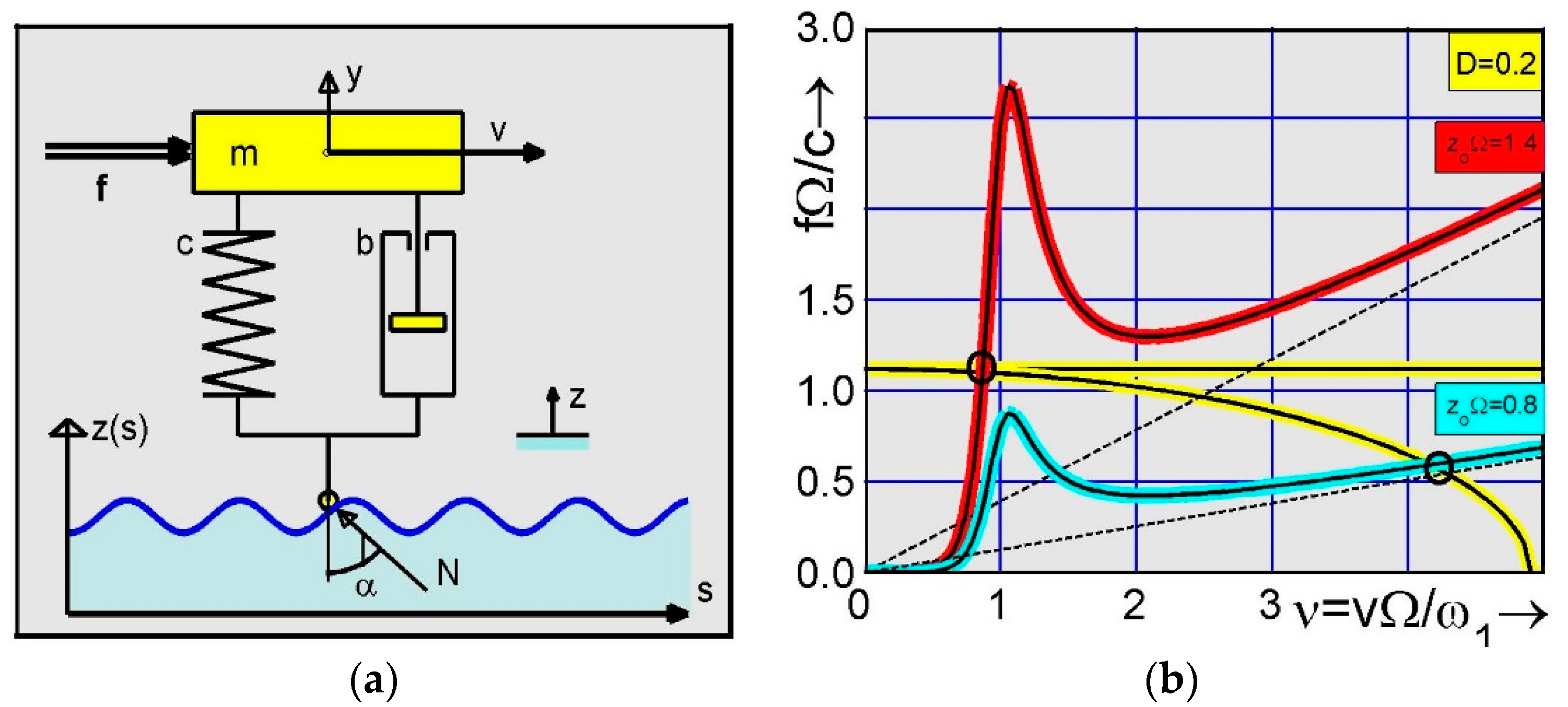
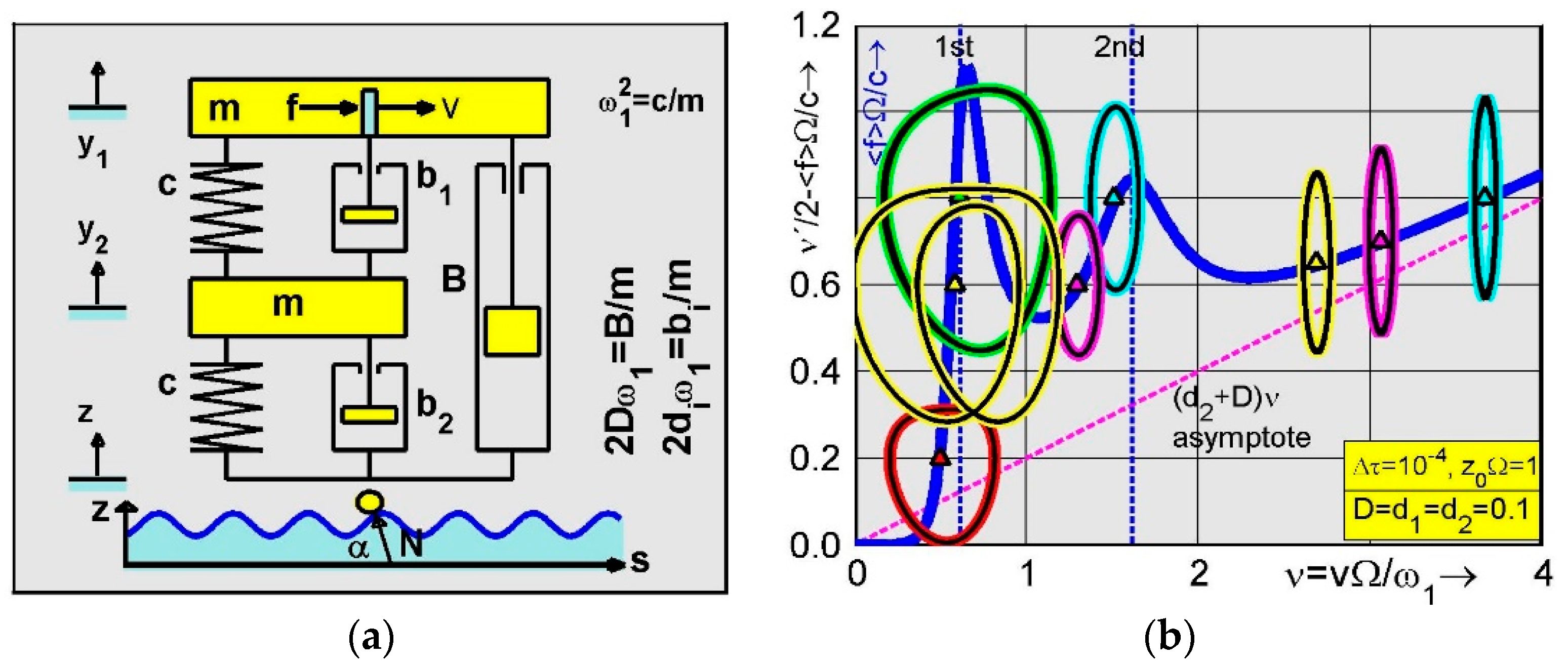
Figure 1a shows the applied quarter car model rolling on a wavy road with vertical displacement
and derivative
taken along the travel way
. In the following, the quantities
and
are called road level and slope, respectively. They generate vertical car vibration displacement
and velocity
, which are coupled by the vehicle speed
and described by the two equations of motion
where
s is the travel displacement of the vehicle and
denotes the coordinate of the vertical vibration velocity. In Equations (1) and (2), dots denote derivatives with respect to time
t. The parameter
determines the natural frequency
of the vertical vehicle vibrations,
denotes the damping, and
is the driving force which is constant or slightly decreasing with growing speed. In
Figure 1b, both force characteristics are plotted in yellow-black. In the following, constant driving force is applied only. The nonlinear term in Equation (1) represents the damper and spring force multiplied by
that takes the horizontal component of the contact force
by means of
One finds Equations (1) and (2) already in the literature in [
13,
14] and in [
2,
3,
4,
5,
6,
7].
In first investigations, the road level and slope are assumed to be sinusoidal as
where
is the amplitude of the road surface and
is the angular spatial frequency determined by the wave length
of the road. Equations (1)–(3) represent a DA equation system where the role of algebraic terms is taken by sinusoidal terms. To eliminate these terms, the road level
and slope
in Equation (3) are differentiated with respect to the way coordinate
in order to obtain the increments
and
that leads to the homogeneous nonlinear oscillator equations
which are obtained when both increments above are divided by
and
is replaced by the speed v. Furthermore,
holds so that Equation (1) reads as
Equations (2), (4) and (5) describe a five-dimensional problem with five unknowns [
4,
7]: the horizontal travel speed
of the vehicle, its vertical vibration by displacement
and velocity
, and the road level
and slope
. For analytical and numerical investigations, it is appropriate to introduce the dimensionless time
and the related speed
, as well as the related coordinates
and
. Their insertion into Equations (2), (4) and (5) leads to
where prime denotes differentiation with respect to the dimensionless time
To improve numerical integration [
2,
7] in Equations (6)–(8), the polar coordinates
are introduced into the road Equation (7) that leads to the transformation equations
which are solved by means of the determinant
and Cramer’s rule to
Without loss of generality, the related polar radius is integrated to Note that the derivative of the polar angle is equal to the negative speed of the vehicle. According to the definition of polar coordinates, the polar angle turns counterclockwise into the mathematically positive direction. The applied oscillator, however, rotates clockwise. This is the reason why both quantities have opposite signs.
3. Speed Driving Force Characteristic of Traveling Vehicles
In order to derive the driving force speed characteristic, shown in
Figure 2, the equations of motion are approximately investigated assuming that the oscillating speed of the vehicle can be averaged by
In this case, the sinusoidal solutions
are applicable and inserted into Equation (8) in order to obtain the matrix equation
applying the coefficient comparison. The first two rows of this matrix equation yield
and
. Both relations are inserted into the last two rows, obtaining
This reduced equation system possesses the determinant
. It is solved by Cramer’s rule in order to obtain first
and then
, as follows:
These results coincide with the linear theory of a constant vehicle speed. They are inserted into the velocity Equation (6) to calculate the time dependent driving force
which is needed to keep the speed
constant. Its mean value is calculated as
The approximated force speed characteristic in Equation (12) is plotted in
Figure 1b for the two road surface parameters
, marked by red and cyan lines, respectively. The dashed line represents the asymptote
, which is proportional to the speed, indicating that one needs a linearly growing driving force to reach higher speeds of operation. Obviously, the increasing driving force is needed to compensate the energy loss in the damper, which is growing with higher speeds, as well.
The force speed characteristic (12) represents a linear approximation obtained by averaging the oscillating driving speed. In order to check the validity and stability of the result in Equation (12), numerical simulations are performed by applying the Euler scheme to
where the related level and slope of the road surface are given by
and
dependent on the polar angle
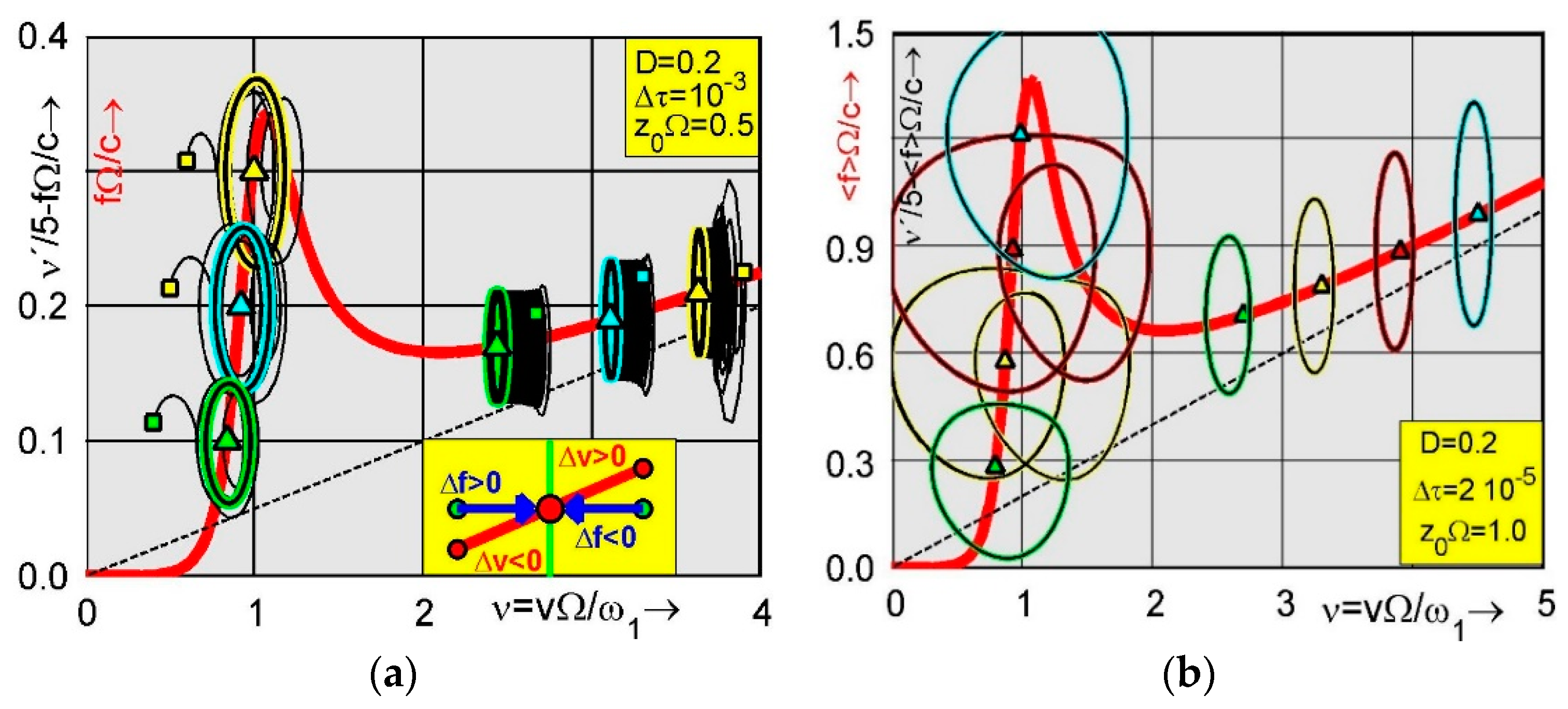
, the derivative of which is equal to the negative speed of the vehicle. The numerical results obtained are presented in
Figure 2a by plotting the scaled and shifted acceleration of the vehicle against the true speed where squares denote initial values of acceleration and speed; triangles are mean values of acceleration and speed calculated after the initially transient period, providing a sufficiently long time for the averaging procedure. In
Figure 2b, stationary limit cycles are shown for a stronger road excitation given, e.g., by
, which leads to the road amplitude
, e.g., for the wave length
Note that phase portraits of velocity over displacement are not applicable for the travel kinematics since the horizontal displacement of the traveling vehicle is growing infinitely. Instead of phase portraits of displacement and velocity,
Figure 2b shows limit cycles of velocity against acceleration. Obviously, there are two speed regions where the limit cycles are stable; the first is in the under-critical speed range before the resonance speed
The second is far beyond the resonance in the higher speed range of operation. In between both stable speed ranges, the slope of the speed driving force characteristic is negative. In this range, limit cycles are not stable and therefore not realizable. This instability is plausible and physically explained inside the yellow area shown in
Figure 2a. Accordingly, a speed perturbation by means of
into the negative speed direction on the left side of the dynamic equilibrium generates an acceleration back to the equilibrium since the applied force
is larger than that one being necessary in the new perturbed situation. In this case the positive driving force difference is equal to the vertical distance between the green and red circle. However, the vehicle is braked if the speed perturbation goes into the positive speed direction on the right side of the dynamical equilibrium. In this case, the applied driving force is smaller than the one necessary to maintain the new perturbed dynamic equilibrium, marked by the right red circle. Vice versa, a speed driving force characteristic with negative slope leads to monotonous instability with the effect that speed leaves the unstable branch. In
Section 5, it is shown that the negative slope condition coincides with the instability in mean, which is derived by applying the Hurwitz criterion to the variational equations of the averaged equations of motion.
Figure 2a shows three limit cycles in the stable under-critical speed range for the driving forces:
marked by green, cyan, and yellow triangles, respectively. The limit cycles are obtained by plotting the scaled and shifted acceleration against the true travel speed. The selected initials are marked by colored squares. Thin black lines are transients which start in the squares and end in the thick colored lines of the one-periodic limit cycles. After this initial period, the simulation is continued a sufficiently long time in order to calculate the mean values of speed and acceleration, which are plotted marked by colored triangles. Obviously, the triangles showing speed and acceleration coincide with the initial values of the applied speed driving force characteristic. Since the accelerations are shifted upward by the applied value of the speed driving force characteristic, the acceleration mean value is vanishing when both triangles coincide. The same property is obtained in the stable region of super-critical speeds
where three one-periodic limit cycles are shown on the right side in
Figure 2a. Again, the transients are marked by thin black lines. After a sufficiently long initial time, the transients go over to the stationary limit cycles marked by green, cyan, and yellow.
In
Figure 2b, the applied wave parameter is doubled by
with the consequence that the amplitudes of the speed oscillations become much broader. Moreover, the one-periodical limit cycles bifurcate into double-periodic ones when for growing driving force the vehicle becomes stuck in the under-critical speed range. This bifurcation scenario is demonstrated by the green limit cycle obtained (left side,
Figure 2b) for the related driving force
which goes over to the yellow double-periodic one if the related force is increased to
For the further increased driving force
, the calculated limit cycle is still double-periodic marked by red and bifurcates back into the one-periodic limit cycle marked by cyan if the driving force is again increased to
For further growing driving force, the resonance speed
is reached with strong oscillations in the vertical and horizontal direction and then passed up to high speed ranges where the driving force can be again decreased. Associated limit circles are single periodic as shown in the right side of
Figure 2b. They are obtained for
marked by green, yellow, red, and cyan, respectively. Correspondingly, colored triangles represent the averaged travel speeds together with the applied driving force. The applied vehicle damping is
and the time step of integration is
Note that for
two different limit cycles are obtained: the first in the under-critical speed range and the second one in the upper-critical speed range. Both are marked by red. In between both stable limit cycles, there is a middle one which is unstable und therefore not realizable. Note that one finds the same behavior in rotor dynamics, where the Sommerfeld rotor leads to the same driving characteristic [
2] when in Equation (12) the road factor
is replaced by the mass ratio of the unbalanced rotor, the translation velocity by the rotation speed ratio, and the driving force by the moment. More details on Sommerfeld effects in rotor dynamics are given in [
16,
17,
18,
19,
20].
4. Stable and Unstable Oscillation Amplitudes of Vehicle Speeds
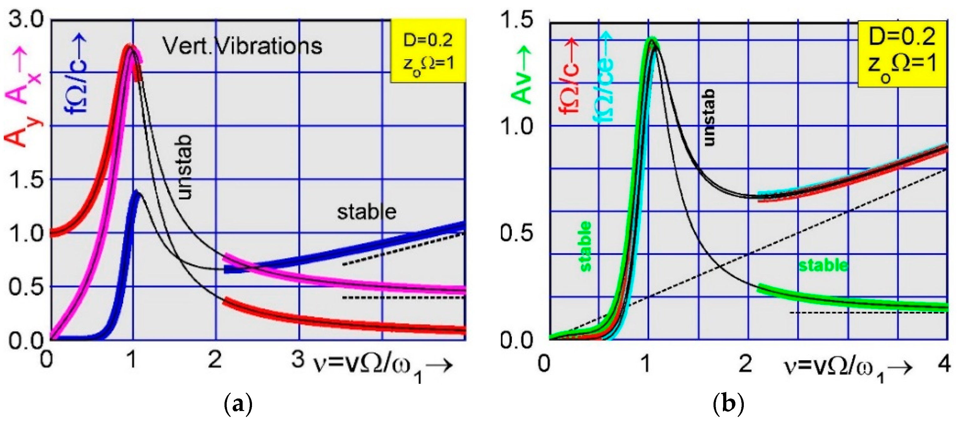
In
Figure 3a, the vibration amplitudes of the vertical displacement (red) and velocity (pink) of the vehicle are plotted against the travel speed together with the speed driving force characteristic shown in blue. The displacement and velocity amplitude are
respectively, where the coefficients
are determined by Equations (10) and (11). The blue curve in
Figure 3a represents the speed driving force characteristic dependent on speed. As already derived, stable travel speeds are only realizable in those speed regions where the slope of the characteristic is positive marked by thick blue lines in the under- and super-critical range. In the middle range, where the slope is negative, the blue curve is replaced by a thin black line, indicating that the calculated stationary speed is unstable and therefore not realizable. From this it follows that the calculated amplitudes
of the vertical vibrations of the vehicle are not realizable in the middle speed range, as well. In the super-critical speed range, however, all stationary vibration amplitudes are stabilized with growing speed and end into asymptotes marked by a dashed line, which are linearly growing, constant without increasing and decreasing for the force characteristic, the velocity, and the displacement amplitude, respectively. Obviously, the asymptote of the driving force corresponds to acceleration. Both quantities, force and acceleration, are linearly increasing with growing speed of the vehicle.
In order to introduce efficient solution methods, the time increment
in Equations (6) and (8) is eliminated by the angle increment
that leads to the time-free equations
where prime in
is replaced by a circle in
denoting differentiation with respect to the polar angle
In Equations (15) and (16), the related road level and slope are sinusoidal and dependent on the polar angle
Accordingly, the vertical vehicle vibrations and the longitudinal speed oscillations are calculable inside one period by means of shooting methods to obtain numerical solutions for
. The associated characteristic multipliers
are investigated by means of the new equation system
which is obtained when the perturbations
and
are inserted into Equations (15) and (16) and the perturbation equations are linearized in the
quantities. According to the Floquet theory, the calculated periodic solutions are asymptotically stable with respect to
if all multipliers
satisfy
For known velocity
, the applied polar angle can be integrated back to time by which the sequence of associated time distances is determined. Note that the four-dimensional time system (13) and (14) is not ergodic since the polar angle
is a state variable that grows infinitely by permanent rotation. This disadvantage is avoided by eliminating the time variable by means of the polar angle, which leads to the three-dimensional angle system (15) and (16) where the polar angle now represents the independent integration variable restricted to one-periodic interval. The solutions of this new time-free equation system are ergodic, and multiplicative ergodic theorems are applicable in order to calculate characteristic numbers of the dynamic system of interest.
For the new angle Equations (15) and (16), new analytical solutions are derived by means of the introduction of the Fourier expansions
where the zeroth Fourier coefficient
of the speed expansion in Equation (19) takes the role of the averaged speed
in
Section 3. The insertion of the expansions (17) and (18) into Equation (15) and the coefficient comparison of the sinusoidal terms of
and
leads to the same result, already noted in Equations (10) and (11). All other terms are cutoff and can only be taken into account when higher expansions are introduced. The insertion of the expansions (17), (18), and (19) into the speed Equation (16) and the coefficient comparison leads to
which represent new results for the amplitudes of the travel speed oscillations. In
Figure 3b, the resultant speed amplitude
is plotted against the mean speed
by
and marked by a thick green line. Obviously, the speed amplitude vanishes if the vehicle slows. It is increasing up to the resonance speed and decreases again for further growing speed, up to the asymptote given in Equation (22). In addition to the above coefficient comparison of terms with
and
, all terms with
lead to the extended speed driving force characteristic
where the first part coincides with Equation (12) and the second part gives a correction of second order. The extended speed driving force characteristic in Equation (23) is plotted in
Figure 3b. The red line marks the first approximation noted in Equation (12). Its second order approximation, noted in Equation (23), is marked by a thick cyan line. It is close to the red line of the first approximation. Thin black lines represent speed driving force characteristics with negative slope where the calculated solutions are unstable and therefore not realizable.
5. Stability in Mean and Robustness with Regard to Disturbances
Note that the velocity Equation (13) is determined by the products of road level z and slope u multiplied by the two vibration coordinates
and
. These products are called covariances [
2]. They determine the dependency of the response of the system from the road excitation. The application of the product rule of differentiation to the road Equation (7) and the vehicle Equation (8) leads to the covariance equation system
where the related speed
of the vehicle is determined by Equation (13) as
Level and slope of the road are
and
respectively. Again, this is a DA equation system where transcendentals take the role of algebraic terms. For numerical integrations, the sinusoidal terms in Equation (3) are generated by means of the road oscillator, noted in Equation (7). The oscillator is transformed by means of the polar coordinates
which are inserted into Equations (24) and (25). The remaining equation
determines the derivative of the polar angle and couples the polar angle back to the speed of the vehicle.
In order to derive analytical approximations, the averaging method is applied by taking the time mean values
and
in Equations (24) and (25) that leads to
when in Equation (24) for
the first two rows are applied to eliminate
and
Subsequently, the covariances
and
are calculated and inserted into Equation (25)
which finally leads to the same speed driving force characteristic
already noted in Equation (12). Note that the above applied time mean values are exact when the speed of the vehicle is constant. For oscillating speeds, the time mean values are approximations.
Following [
2], the averaged Equation (24) are applied to investigate the stability in mean of the averaged speed by means of the perturbation equation system
which is obtained by means of the perturbations
and
for
. The insertion of the perturbations into the averaged Equations (24) and (25) and linearization in the
-terms yields the fifth order stability Equation (27) with the characteristic equation
The determinant of Equation (27) yields
According to the Hurwitz criterion,
determines divergence that gives the boundary of monotonous instability. Obviously, the stability condition
coincides with the positive slope condition of the speed driving force characteristic calculable by differentiating Equation (12) with respect to the travel speed
that gives
This result coincides with Equation (28) except that the positive definite denominator in Equation (28) is squared. Hence, the negative slope condition and the instability in mean lead to the same instability boundary. This is plausible and physically explainable, as already done in the yellow area in
Figure 2a. The instable speed range vanishes with increasing damping.
In addition to the stability behavior, the robustness of the limit cycle calculation with regard to disturbances is of interest. When disturbances are generated by brief shocks, the eigenvalues of the stability matrix in Equation (27) must be calculated. They determine the growth behavior with which the disturbances increase or decrease, respectively. In the case of stationary disturbances, noise models are introduced.
Figure 4a shows a stochastic limit cycle obtained for the quarter car model in the case that the angle motion on the sinusoidal road form is perturbed by additive noise given by
In Equation (29), capital letters with index
denote set functions [
21,
22] dependent on time. Noise is generated by normally distributed numbers
with zero mean [
23]. The stochastic angle perturbation takes into account that the road surface is no longer sinusoidal but more realistically irregular and noisy with bounded realizations. For small noise intensities
this leads to response realizations which are bounded, as well.
Initial results are shown in
Figure 4a where trajectories of a stochastic limit cycle are plotted in the phase plane of travel velocity and acceleration scaled by 0.3 and shifted by the applied driving force. The realizations are calculated by means of Equations (24)–(26) where the polar angle in Equation (26) is replaced by Equation (29). The applied damping is given by
the driving force by
the road level by
and the noise intensity by
The Euler scheme is applied with the time step
The mean value of the shifted acceleration and true velocity is marked by a yellow triangle on the red curve of the speed driving force characteristic, indicating that the mean acceleration is vanishing and the mean travel speed coincides with Equation (12). The comparison with the double-periodic yellow limit cycle in
Figure 2b shows that its sharp line is widened to a bundle of nonperiodic realizations, the boundaries of which are double periodic with two loops and one node of two crossing limit flows.
Figure 4b shows the associated double-crater-like probability distribution density on the phase plane of velocity and acceleration calculated for the stronger noise intensity
Clockwise rotation in the phase plane of acceleration and true speed is slow when the probability density is high and vice versa fast for low densities. Note that
Figure 4a,b present new results in nonlinear stochastic vehicle dynamics, obtained by applying noise perturbations that are bounded by means of the applied sinusoidal terms. For small intensity σ, the limit flow in
Figure 4a possesses periodic side limits in spite of the fact that all limit cycle realizations are random. This is a new effect presented in this paper. For growing intensity σ, the inner side limits of the limit cycle shown in
Figure 4a become broader and finally disappear, such that only the outer side limits remain, and the whole phase plane in
Figure 4a is covered by realizations of velocity and acceleration.
6. Stable Travel Speeds of Road Vehicle Systems
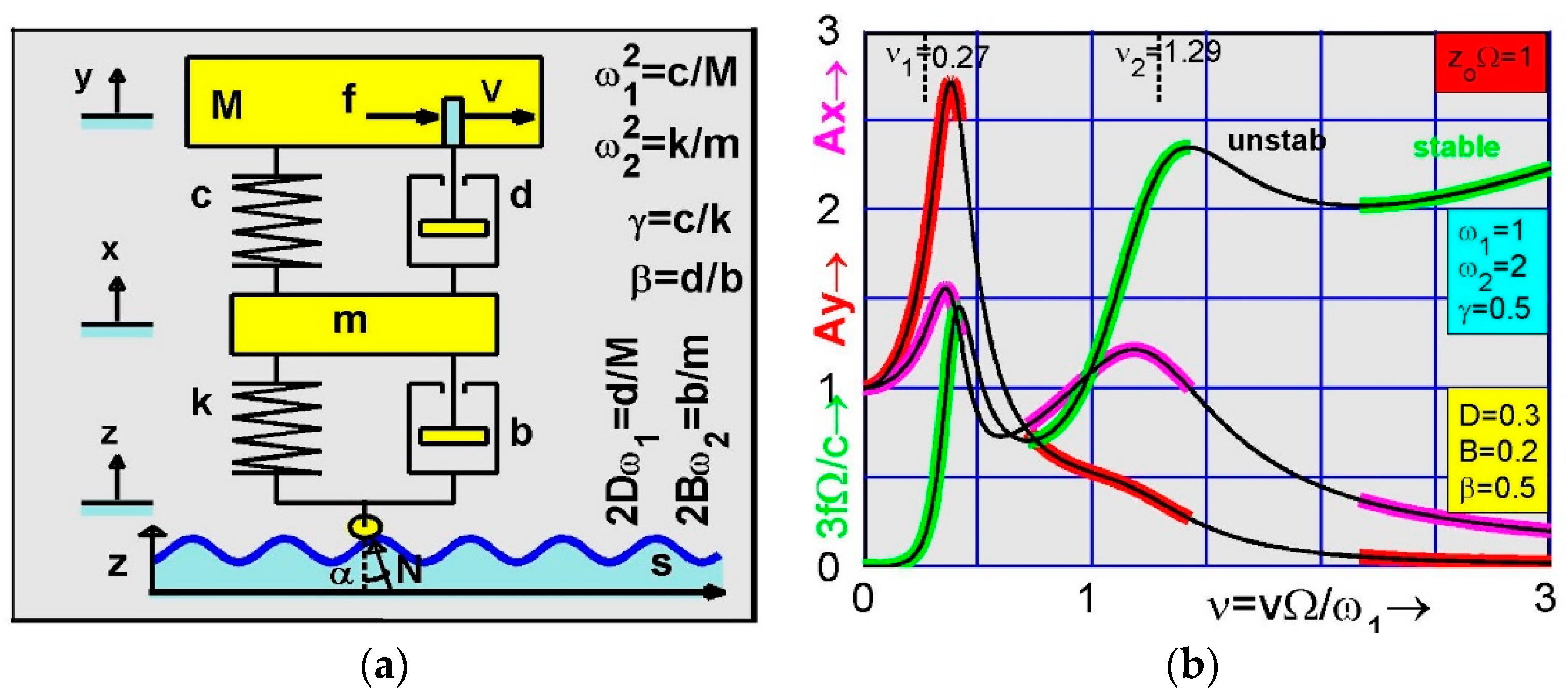
To extend the above investigations to higher order models, consider the quarter car model with two degrees of freedom shown in
Figure 5a. The motions of the car body of mass
and the wheel mass
are described by the equations of motion
where the system frequencies
,
and the damping coefficients
are introduced together with the stiffness and damping ratios
and defined as follows:
The parameter
denotes the stiffness ratio of the car and wheel spring
and
, respectively. Correspondingly,
is the damping ratio of the car and wheel damper
and
, respectively. The reference frequencies
and
describe the decoupled vibrations of the wheel and car body. In addition to Equations (30) and (31), the dynamic balance in horizontal direction gives a third equation of motion that determines the travel speed, as follows:
Note that Equation (32) is of first order with respect to the car speed and s denotes the longitudinal coordinate of the travel path. Note that both masses are assumed to be concentrated in the contact point of road and vehicle so that only planar translations are considered. Rotations are excluded.
It is appropriate to introduce the dimensionless vibration and road coordinates by means of
and
respectively. The insertion of these coordinates into Equations (30) and (31) leads to the dimensionless equations of motion
where
is the related speed of the vehicle rolling on road with level
and slope
In order to derive a first approximation, it is assumed that the oscillating speed of the vehicle can be averaged by
In this case, the travel path is s
and the equations of motion become linear. They are solved by the set-up
In the stationary case, the insertion of these set-ups into Equations (33) and (34) and the coefficient comparison leads to the linear matrix equation
where
is the reference frequency ratio given by
The coefficients
of the sinusoidal set-up are calculated by means of Equation (35) and inserted into
which are plotted in
Figure 5b against the related speed of the vehicle. The amplitude
of the car body is marked by red and the wheel amplitude
by pink. In unstable speed ranges, both amplitudes are marked by thin black lines.
The vertical vibration amplitudes of both masses are calculated for the reference frequencies
for the stiffness-ratio
and for the damping values
and
The applied road wave is chosen by
This is equivalent to the height–length ratio
when the wave frequency
is inserted into
. The frequency responses in
Figure 5b possess two resonance speeds: the first at
and the second at
Both eigenvalues are valid for vanishing damping. In order to decide the realizability of the stationary vehicle speeds applied in Equation (35), the new speed Equation (32) is investigated in the dimensionless form
As already shown in
Section 3, Equation (36) can approximately be evaluated by averaging the oscillating speed with
and introducing the time mean values
and
into Equation (36). This gives the new approximated force characteristic
where
and
are calculated by means of Equation (35). New numerical evaluations of Equations (35) and (37) are plotted in
Figure 5b and marked by green for stable speeds when the slope of the speed driving force characteristic is positive and by black-thin lines when the slope is negative. In the latter case, the speed applied in Equation (35) is unstable and physically not realizable. Finally, it is noted that both instability speed ranges are vanishing for growing damping coefficients.
The instability behavior is numerically investigated by means of simulations applied to a slightly modified quarter car model with two equal masses
m and a third damper
, as shown in
Figure 6a. The car is rolling with velocity
on a wavy road described by
in dependence on the travel way coordinate
. The speed frequency
is related to the reference frequency
given by
. The vertical vibrations of this car model are described by the two nonlinear equations of motion
where
couples both vertical vibrations to the horizontal velocity described by
The damping coefficients are introduced by for For numerical integration, the dimensionless time and the velocity together with the related coordinates and are inserted into the velocity Equation (40) and vehicle Equations (38) and (39).
Figure 6b shows the average vehicle speed for a given driving force
, marked by a blue thick line. It is calculated for the road level
and the damping values
. In the middle range of the related driving force
, there are five branches of stationary solutions: two solution branches are unstable and three are stable. The stable speeds possess positive slopes in the driving force speed characteristic; meanwhile, speeds started in negative slope ranges do not remain in this range. They migrate to higher or lower speed ranges.
Figure 6b shows three limit cycles (red, yellow, green) before the first resonance, two further limit cycles (red, cyan) between the first and second resonance and the last three limit cycles for overcritical speeds near the asymptote
which is marked by a dashed red line. Mean values of shifted acceleration and true speed are plotted by colored triangles on positive slopes.

