Article

Stabilization of the Magnetic Levitation System

Faculty of Electrical Engineering and Information Technology, Slovak University of Technology in Bratislava, Ilkovičova 3, 812 19 Bratislava, Slovakia
*
Author to whom correspondence should be addressed.
Appl. Sci. 2021, 11(21), 10369; https://doi.org/10.3390/app112110369
Submission received: 10 August 2021 / Revised: 28 October 2021 / Accepted: 29 October 2021 / Published: 4 November 2021
(This article belongs to the Special Issue New Trends in Automation Control Systems and Their Applications)

Abstract

:
This paper contributes toward research on the control of the magnetic levitation plant, representing a typical nonlinear unstable system that can be controlled by various methods. This paper shows two various approaches to the solution of the controller design based on different closed loop requirements. Starting from a known unstable linear plant model—the first method is based on the two-step procedure. In the first step, the transfer function of the controlled system is modified to get a stable non-oscillatory system. In the next step, the required first-order dynamic is defined and a model-based PI controller is proposed. The closed loop time constant of this first-order model-based approach can then be used as a tuning parameter. The second set of methods is based on a simplified ultra-local linear approximation of the plant dynamics by the double-integrator plus dead-time (DIPDT) model. Similar to the first method, one possible solution is to stabilize the system by a PD controller combined with a low-pass filter. To eliminate the offset, the stabilized system is supplemented by a simple static feedforward, or by a controller proposed by means of an internal model control (IMC). Another possible approach is to apply for the DIPDT model directly a stabilizing PID controller. The considered solutions are compared to the magnetic levitation system, controlled via the MATLAB/Simulink environment. It is shown that, all three controllers, with integral action, yield much slower dynamics than the stabilizing PD control, which gives one motivation to look for alternative ways of steady-state error compensation, guaranteeing faster setpoint step responses.

1. Introduction

The magnetic levitation system represents a typical nonlinear unstable system. Since it presents several interesting problems for control, there exists numerous educational laboratory models that can be used for verifying control algorithms, demonstrating their properties. The most used are products from Quanser [1], Humusoft [2], Googol [3], LD Didactic Group [4], and Inteco [5].
For controlling the position of the ball in the magnetic field created by the solenoid, the system enables using a wide variety of methods, such as:
  • polynomial approach [6,7,8];
  • LQR PID tuning [9];
  • constrained control [10,11];
  • robust control [12];
  • model predictive control; [11,13,14];
  • state space control [15,16];
  • direct synthesis method for stable and unstable systems [17,18];
  • fuzzy control [19,20].
The paper presents and compares two possible solutions to the magnetic levitation plant control problem.
The first method is based on the knowledge of the transfer function of the linearized system (1) derived, considering parameters given by the manufacturer [21]. It starts with stabilizing the given unstable system. In the next step, the dynamics of compensation of the emerging disturbances are specified. By neglecting the fast stable mode of transients, the design procedure can be made simple and robust, similar to model-based PI control [22]. The controllers designed by the first approach make it possible to measure the input–output steady-state characteristic (IOSSCH) of the system, expressing the dependence of the output variable of the system on the input in steady states (Figure 2). While the analytically derived transfer function of the system results in a linear dependence of the output from the input at steady states, the measured dependence shows non-linear properties of the system. It indicates that, in an effort to accelerate transients by this approach, we would have to deal with the limited accuracy of the linear model. Although the proposed control meets most of the above requirements, it will be relatively slower in terms of transient speed.
Therefore, to verify the plant dynamics, the second group of possible approaches begins with identifying the system. The authors of [10] have already pointed out several aspects that are important in the effort to achieve the fastest possible (and sufficiently smooth) transients at the input and output of the system. In view of the non-linearity of the system, in the second set of approaches, it is preferred to approximate the system’s dynamics by means of the simplest second-order transfer function of a double integrator with a transport delay (DIPDT, double integrator plus dead time). Such an ultra-local model, typical of today’s popular robust control approach with active disturbance rejection control (ADRC) [23,24,25,26,27], avoids the need to approximate nonlinear system feedback. A similar simplification is used by another method working with finite impulse response (FIR) filters. Due to omitting identification of internal plant feedback, it is also called model-free-control (MFC). Its application can lead to an intelligent proportional-derivative (iPD) controller [28,29,30,31]. After determining the DIPDT plant model, simple proportional-derivative (PD) controllers can be used for the stabilizing controller design [31,32]. When supplemented by low-pass filter design and combined with static feedforward (using inversion of the measured IOSSCH), it is possible to get control processes that are already very close to the performance limits given by the available hardware. To deal with possible disturbances (including the model imperfections), the proportional-integral-derivative (PID) controllers (supplemented again by the design of low-pass filters [33]), or internal model control (IMC) controllers may be added to the basic loop with a stabilizing PD controller [34]. However, the achieved controllers with integral (I) action again show much slower dynamics than the simple stabilizing PD controller with the offset compensation by static feedforward.
The rest of the paper is structured as follows. Section 2 briefly describes the magnetic levitation system. In Section 3, a simplified controller design is presented that, after stabilizing the system and neglecting the fast stable mode of transients, can be denoted as a model-based PI controller design. In Section 4, three different controllers are presented, based on the simplest plant approximations by the time-delayed double-integrator plus dead-time (DIPDT) model.The achieved results are discussed and summarized in the Conclusions. The main contribution of the article can be considered the analysis and experimental verification of several possible features of the design of the rapid nonlinear and unstable process of magnetic levitation, with regard to the most frequently placed requirements. It follows that, all used controllers with I action finally give dynamics, which is significantly slower than with simple stabilizing PD controllers. This provides an incentive for further work to explore new alternatives, to eliminate permanent control-error without significantly reducing the dynamics of the setpoint responses.

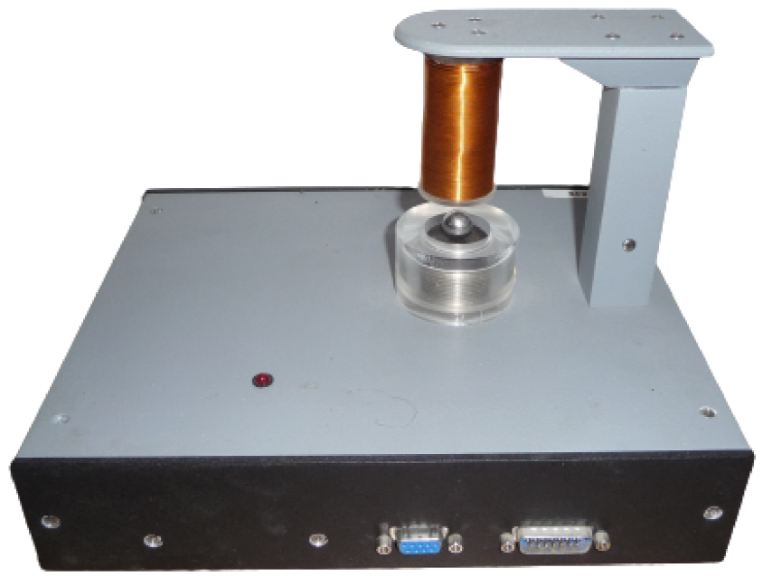
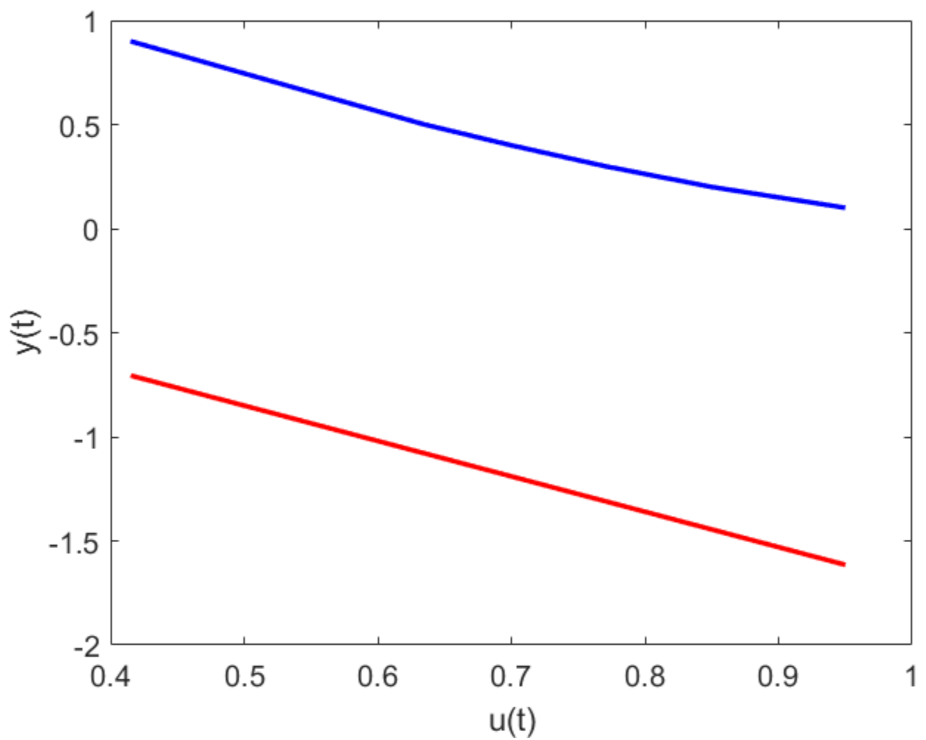
2. Magnetic Levitation Plant

The paper deals with the control of the magnetic levitation plant CE152, provided by Humusoft ([2], see Figure 1). This educational laboratory model enables demonstrating control problems associated with nonlinear unstable systems. The aim is to stabilize and control the ball position. The company originally supported communications via the MF624 A/D card [35]. To get new degrees of freedom, the MF624 card was substituted by the low cost solution based on the Arduino Due board [36].
The plant is controlled via the MATLAB/Simulink simulation environment that enables running simulations in an external mode. The support for Arduino Due is available thanks to third-party add-ons, called Simulink Support Package for Arduino Hardware.
The literature offers several models that describe the dynamic behavior of the magnetic levitation system. In addition to nonlinear models [37], simplified linear models could also be found.Very often, they are described by the third order system with three time constants (see, e.g., [12,38,39,40]). However, after a more detailed analysis, it can be found that one time constant (electrical) can be neglected in comparison to other two time constants, which are approximately the same in its value, but one pole is positive and one negative. This can be confirmed by the second order models of the Humusoft magnetic levitation plant, published in [6,41] or [13]. Therefore, the magnetic levitation model can be replaced practically in the whole controlled range (approximately 0.1–0.9), which is given by the used sensor (its range is transformed to the so-called 1 M U ), by the transfer function
G ( s ) = K T 2 s 2 1
The correctness of this model is also confirmed by the comparison of the measured input–output characteristic and the characteristic corresponding to the model (1) (Figure 2). Both shapes are very close to each other. Their displacement is due to the asymmetry of the gravitational force not taken into account by the transfer function of the system (1).
As mentioned, the electrical time constant considered in other publications is neglected, because it is small enough compared to the mechanical time constant.

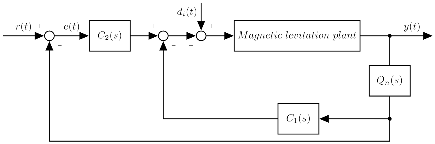
3. Weighted PID Controller Design

As it is possible to see, the transfer function describing the ball movement (1) is unstable. The first step in designing the controller is to stabilize the system. Its desired closed-loop behavior can be expressed using the second order transfer function
M ( s ) = 1 β ( τ 1 s + 1 ) ( τ 2 s + 1 )
The considered structure of the control scheme is shown in Figure 3.
The transfer function C 1 ( s ) represents a controller providing stabilizing feedback
C 1 ( s ) = 1 M ( s ) 1 G ( s )
that for (2) can be written in general form
C 1 ( s ) = a 2 s 2 + a 1 s + a 0
Considering a 2 = 0 , we get a PD controller, whereby the parameter β can be expressed as
β = T 2 K τ 1 τ 2
Transfer function M ( s ) can be reduced to the 1st order by the suitable choice of time constants τ 2 τ 1 , when
M ( s ) 1 β ( τ 1 s + 1 )
This can be achieved, e.g., by defining τ 1 = ρ T and τ 2 = T / ρ where ρ is a sufficiently big value. Then,
β = 1 K
a 0 = β + 1 K = 2 K
a 1 = T K ρ 2 + 1 ρ
After stabilizing the system, it is possible to proceed to the design of the controller C 2 ( s ) , which will ensure the required behavior of the entire control structure under impact of disturbances.
Since the transfer function (6) is first order, the desired closed loop transfer function F ( s ) can also be selected as a first order function
F ( s ) = 1 λ s + 1
Correspondingly, in such a model-based design, the transfer function of the controller
C 2 ( s ) = F ( s ) 1 F ( s ) 1 M ( s )
remains feasible. Considering (10) a (6),
C 2 ( s ) = ρ T K λ + 1 K λ s = ρ T K λ 1 + 1 ρ T s
It is obvious that this is the structure of the PI controller
C 2 ( s ) = K C 1 + 1 T I s ; K C = ρ T K λ ; T I = ρ T
the gain of which can be influenced by the choice of λ . For λ = ρ T je K C = 1 / K .
The considered control structure (Figure 3) still contains one block and it is the first order filter Q ( s )
Q ( s ) = 1 T f s + 1
Its aim is to ensure filtering of the measured signal.

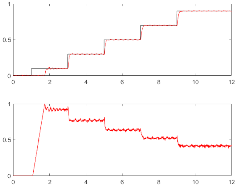
Experimental Results

The whole design was accomplished considering parameters in Table 1.
These parameters lead to the following values β = 0.588 , a 0 = 1.177 a, a 1 = 0.027 s. For λ = ρ T = 0.036 s, the controller parameters are K C = 0.588 a, T I = 0.036 . In the experiment, the sampling period was 1 ms and the time constant of the filter Q ( s ) was equal to the sampling period. A corresponding transient and control signal is shown in Figure 4.
The advantages of this approach are its simplicity, high robustness, and low sensitivity to measurement noise.

4. Multiple Real Dominant Pole Controller Design

The multiple real dominant pole (MRDP) controllers rely on the DIPDT model of the magnetic levitation plant F ( s )
F ( s ) = K s s 2 e T d s
with parameters identified in [10], by means of step responses, as
F ( s ) = K m s 2 e T m s ; K m = 7000 ; T m = 0.002   s

4.1. PD Controller Design by the Triple Real Dominant Pole Method

The considered control structure is shown in Figure 5. In this case, the stabilizing PD controller
C 0 ( s ) = K p + K d s
will be combined with a second order low-pass filter
Q 2 ( s ) = 1 T f s + 1 2 .
Then
C ( s ) = C 0 ( s ) Q 2 ( s )
In the controller tuning, its two time constants T f will be considered by the modified half-rule method [33,42], as an amendment to the total dead-time by an equivalent filter dead-time T e
T d = T m + T e ; T e = 2 T f / 2 = T f .
Thus, it can be omitted from further derivations. The control structure segments with the transfer functions C 1 ( s ) , C 2 ( s ) , and C 3 ( s ) will be omitted by choosing C 1 ( s ) = 1 and C 2 ( s ) = C 3 ( s ) = 0 .
The PD control combined with a DIPDT plant yields a closed loop transfer function
F w y ( s ) = Y ( s ) W ( s ) = K s ( K d s + K p ) e T d s s 2 + K s ( K p + K d s )
As shown, e.g., in [31,32], for the characteristic polynomial
A P D ( s ) = e T d s s 2 + K s ( K p + K d s ) ,
a triple-real-dominant-pole (TRDP) s o corresponds to a tuning, satisfying conditions:
A P D ( s ) ; d A P D s d s ; d A P D 2 s d s 2 s = s o = 0
From
d A P D 2 s d s 2 = ( T d 2 s 2 + 4 T d s + 2 ) e T d s = 0
follows the TRDP as
s o = E / T d ; E = 2 2
where appropriate, the triple closed-loop time constant
T o = 1 / s o = 1.707 T d
can be used to characterize the speed of the responses. The corresponding optimal PD controller tuning can then be specified by the gains
K p 0 = ( 10 E + 6 ) e E K s T d 2 = 0.079 K s T d 2 ; K d 0 = 2 ( E + 1 ) e E K s T d = 0.461 K s T d
To compensate the dominant input disturbance caused by the gravitation force, and leading to a significant steady-state error, a simple static feedforward can be used based on the inverse IOSSCH, given as u f f = f 1 ( r ) , where y s s = f ( u s s ) is IOSSCH. In the simplest case, it may be approximated by the slope K 1 and the offset K 2 . These values can be found after approximating IOSSCH by straight-line dependence and determining its slope ( K 1 ) and y-intercept ( K 2 ).
Another alternative is to use static feedforward via inversion of the measured IOSSCH approximated by a lookup table in MATLAB/Simulink. In such a case, in the control structure in Figure 5, the block K 2 is omitted and the block K 1 replaced by the inverse IOSSCH (see Figure 6).
The corresponding step responses in Figure 7 and Figure 8 show much faster responses than with the first method. The steady-state control error can be eliminated by a more accurate inverse IOSSCH approximation for lower reference signal values, extended possibly by gain-scheduling, modifying the K m value, depending on the reference setpoint r. However, when the circuit properties change (e.g., by increased coil temperature), the used control structure is not able to change its properties, and a permanent error may reappear again.

4.2. IMC Control of the Stabilized Plant

Based on the plant stabilized by the above PD controller, several approaches can be proposed. From the real dominant pole and the time constant (25) and (26), it is possible to get a stabilized closed-loop approximation
S s o ( s ) = s o 3 ( s s o ) 3 = 1 ( 1 + T o ) 3 ; s o = E / T d ; E = 2 2 ; T o = 1.707 T d
which may then be used by the IMC control structure in Figure 5 with C 3 ( s ) = 1 , with the plant model and the controller
C 1 ( s ) = ( 1 + T o s ) 3 ( 1 + T c s ) 3 ; C 2 ( s ) = S s o ( s ) = 1 ( 1 + T o s ) 3 ; T o = 1.707 T d
represents a filtered inversion of S s o ( s ) with the required closed-loop time constant T c . Since the transfer function (28) represents just an approximation of the loop stabilized with the PD controller, in order to get reliable results, it is necessary to choose
T c > > T o .
For the model parameters (16) T o = T m / ( 2 2 ) = 0.0034 s, and the choice T c = 0.1 s, the resulting transients in Figure 9 guarantee zero permanent control error, but with regard to the requirement (30), they are significantly slower than when using just a stabilizing PD controller.
The method could also be modified in such a way that the design of the IMC structure would be based on the transfer functions of the stabilized circuit identified experimentally, e.g., by using some step-response-based method.

4.3. Direct PID Controller Design

Approximation of the plant dynamics by the DIPDT model (15) with the parameters (16) can also be used for a direct PID controller design, yielding
C ( s ) = U ( s ) Y ( s ) = K C 1 + 1 T I s + T D s
To get a feasible transfer function with a satisfactory noise attenuation, it has to be combined with a second order filter
C ( s ) Q 2 ( s ) = K C T I T D s 2 + K C T I s + K C s T I T f 2 s 2 + 2 T f s + 1
To avoid output overshooting in step responses, the controller should be extended by a pre-filter (see Figure 10)
N ( s ) = 1 T I T D s 2 + T I s + 1
To achieve uniform starting points of comparison, we again implement the design of optimal parameters using the multiple real dominant pole method. Following [33], to get a four-tuple real dominant closed loop pole s o (time constant T o )
s o = 0.416 / T d ; T o = 1 / s o = 2.404 T d
the controller parameters should be chosen as
K C = 0.125 K s T d 2 T I = 10.324 T d T D = 4.043 T d
The filter dynamics can again be considered by an equivalent delay (20). The PID controller proportional gain K C is now significantly higher than K p 0 of PD controller (27), which, together with increased derivative gain K D = K C T D = 0.505 / ( K s T d ) , lead to increased sensitivity to the measurement noise and plant model imperfections of the transients in Figure 11.
Compared to the dominant closed-loop time constant T o = 1.707 T d of the circuit with PD controller, the dominant time constant T o = 2.404 is now 1.41 times larger and also due to the increased order of the dominant pole the transients will be significantly slower. Thus, also in this situation, the comparison with a simple stabilizing PD controller shows that it might be interesting to examine its use in combination with some alternative permanent control error elimination, allowing achievement of faster transients, which was not possible when using existing hardware.
Simulation verifications show that, in order to achieve improved performance with this design method, the sampling period should be significantly reduced.

5. Conclusions

This paper illustrated two different approaches to the control of the magnetic levitation plant based on different linear plant models.
The first one, based on the transfer function of the underdamped second order model, shows a method that is very easy for use. Connection of controllers C 1 ( s ) and C 2 ( s ) to one block would result to the weighted PID controller. The output of the presented design procedure is the resulting controller structure, controller parameters ( K C , T I , T D ) as weights of signals. The use of a more complex filter and the use of a PID controller instead of a PI controller in the direct branch of the scheme could lead to faster transient responses. Thereby, the position sensor properties (response time ≈ 1 V/1 ms) would act as limiting factors of the control structure. Under control with integral action, elimination of these limitations would only be possible by increasing the flow of information from the process by using a shorter sampling period, which was not experimentally possible with the existing hardware.
Similar results have been achieved by considering two alternative controllers with integral action based on the DIPDT model, identified in [10]. Otherwise, the speed of transients can only be increased by simpler PD control without I-action, at the cost of a possible permanent steady-state error. Such a conclusion raises the question as to whether the elimination of the permanent control error cannot be achieved in combination with a stabilizing PD controller, and some other method that would not lead to such a significant slowdown of processes.

Author Contributions

Writing-original draft preparation, M.H., Š.C. and K.Ž. Simulations, M.H. Experiments, Š.C. and K.Ž. Editing, M.H., Š.C. and K.Ž. Project administration, K.Ž. All authors have read and agreed to the published version of the manuscript.

Funding

This research was funded by the following grants—APVV SK-IL-RD-18-0008 platoon modeling and control for mixed autonomous and conventional vehicles: a laboratory experimental analysis, VEGA 1/0745/19 control and modeling of mechatronic systems in e-mobility, and KEGA 030STU-4/2021 building of mechatronic laboratory using smart technologies.

Institutional Review Board Statement

Not applicable.

Informed Consent Statement

Not applicable.

Data Availability Statement

Not applicable.

Conflicts of Interest

The authors declare no conflict of interest.

References

  1. Quanser. Magnetic Levitation. Available online: https://www.quanser.com/products/magnetic-levitation/ (accessed on 4 August 2021).
  2. Humusoft s.r.o. CE152 Magnetic Levitation Model. Available online: https://www.humusoft.cz/models/ce152/ (accessed on 20 July 2019).
  3. Googol Technology Ltd. Magnetic Levitation System. Available online: http://www.googoltech.com/pro_view-67.html (accessed on 4 August 2021).
  4. LD Didactic Group. E6.3.5.14 Magnetic Levitation. Available online: https://www.ld-didactic.de/phk/gruppen.asp?PT=VE6.3.5.14&L=2 (accessed on 4 August 2021).
  5. INTECO. Magnetic Levitation Systems. Available online: http://www.inteco.com.pl/products/magnetic-levitation-systems/ (accessed on 4 August 2021).
  6. Gazdoš, F.; Dostál, P.; Pelikán, R. Polynomial approach to control system design for a magnetic levitation system. Cybern. Lett. 2009, 7, 1–19. [Google Scholar]
  7. Jen, C.H.; Jiang, B.C.; Fan, S.K.S. General run-to-run (R2R) control framework using self-tuning control for multiple-input multiple-output (MIMO) processes. Int. J. Prod. Res. 2004, 42, 4249–4270. [Google Scholar] [CrossRef]
  8. Fan, S.K.S.; Jiang, B.C.; Jen, C.H.; Wang, C.C. SISO run-to-run feedback controller using triple EWMA smoothing for semiconductor manufacturing processes. Int. J. Prod. Res. 2002, 40, 3093–3120. [Google Scholar] [CrossRef]
  9. Kumar, E.V.; Jerome, J. LQR based Optimal Tuning of PID Controller for Trajectory Tracking of Magnetic Levitation System. Procedia Eng. 2013, 64, 254–264. [Google Scholar] [CrossRef] [Green Version]
  10. Huba, M.; Kamenský, M. Constrained Magnetic Levitation Control. IFAC Proc. Vol. 2005, 38, 901–906. [Google Scholar] [CrossRef] [Green Version]
  11. Fan, S.K.S.; Lin, Y. Multiple-input dual-output adjustment scheme for semiconductor manufacturing processes using a dynamic dual-response approach. Eur. J. Oper. Res. 2007, 180, 868–884. [Google Scholar] [CrossRef]
  12. Hypiusová, M.; Kozáková, A. Robust PID controller design for the magnetic levitation system: Frequency domain approach. In Proceedings of the 21st International Conference on Process Control (PC), Štrbské Pleso, Slovakia, 6–9 June 2017; pp. 274–279. [Google Scholar] [CrossRef]
  13. Chalupa, P.; Novák, J.; Malý, M. Modelling And Model Predictive Control Of Magnetic Levitation Laboratory Plant. In Proceedings of the 31st European Conference on Modelling and Simulation (ECMS), Budapest, Hungary, 23–26 May 2017; pp. 367–373. [Google Scholar] [CrossRef] [Green Version]
  14. Rušar, L.; Krhovják, A.; Bobál, V. Predictive control of the magnetic levitation model. In Proceedings of the 2017 21st International Conference on Process Control (PC), Štrbské Pleso, Slovakia, 6–9 June 2017; pp. 345–350. [Google Scholar] [CrossRef]
  15. Barie, W.; Chiasson, J. Linear and nonlinear state-space controllers for magnetic levitation. Int. J. Syst. Sci. 1996, 27, 1153–1163. [Google Scholar] [CrossRef]
  16. Lee, T.E.; Su, J.P.; Yu, K.W. Implementation of the State Feedback Control Scheme for a Magnetic Levitation System. In Proceedings of the 2007 2nd IEEE Conference on Industrial Electronics and Applications, Harbin, China, 23–25 May 2007; pp. 548–553. [Google Scholar] [CrossRef]
  17. Chamraz, Š. Design of the position controller using the generalized method of required dynamics. J. Cybern. Inform. 2010, 11, 32–40. [Google Scholar]
  18. Chamraz, Š. Controller Design Based on Direct Synthesis and Disturbance Rejection. In Proceedings of the 10th International Conference Process Control; University of Pardubice: Kouty nad Desnou, Czech Republic; 2012. [Google Scholar]
  19. Farana, R.; Walek, B.; Janosek, M.; Zacek, J. Advantages of Fuzzy Control Application in Fast and Sensitive Technological Processes. Int. J. Electr. Comput. Eng. 2015, 9, 1270–1274. [Google Scholar] [CrossRef]
  20. Hamed, B.; Elreesh, H.A.; Balakrishnan, P.; Molhem, M. FPGA Optimized Fuzzy Controller Design for Magnetic Ball Levitation using Genetic Algorithms. ACEEE Int. J. Electr. Power Eng. 2012, 10, 72–81. [Google Scholar]
  21. Humusoft s.r.o. CE152 Magnetic Levitation Model—Educational Manual; 2002. [Google Scholar]
  22. Skogestad, S. Simple analytic rules for model reduction and PID controller tuning. J. Process. Control 2003, 13, 291–309. [Google Scholar] [CrossRef] [Green Version]
  23. Miklosovic, R.; Gao, Z. A robust two-degree-of-freedom control design technique and its practical application. In Proceedings of the Conference Record of the 2004 IEEE Industry Applications Conference, 2004. 39th IAS Annual Meeting, Seattle, WA, USA, 3–7 October 2004; Volume 3, pp. 1495–1502. [Google Scholar]
  24. Gao, Z. Active disturbance rejection control: A paradigm shift in feedback control system design. Am. Control. Conf. 2006, 2006, 2399–2405. [Google Scholar]
  25. Gao, Z. On the centrality of disturbance rejection in automatic control. ISA Trans. 2014, 53, 850–857. [Google Scholar] [CrossRef] [Green Version]
  26. Zhao, S.; Gao, Z. Modified active disturbance rejection control for time-delay systems. ISA Trans. 2014, 53, 882–888. [Google Scholar] [CrossRef] [Green Version]
  27. Chen, S.; Xue, W.; Zhong, S.; Huang, Y. On comparison of modified ADRCs for nonlinear uncertain systems with time delay. Sci. China Inf. Sci. 2018, 61, 70223. [Google Scholar] [CrossRef] [Green Version]
  28. Fliess, M.; Join, C. Model-free control. Int. J. Control 2013, 86, 2228–2252. [Google Scholar] [CrossRef] [Green Version]
  29. Jiang, N.; Zhang, S.; Xu, J.; Zhang, D. Model-free control of flexible manipulator based on intrinsic design. IEEE/ASME Trans. Mechatron. 2020, 26, 2641–2652. [Google Scholar] [CrossRef]
  30. Fliess, M.; Join, C. An alternative to proportional-integral and proportional-integral-derivative regulators: Intelligent proportional-derivative regulators. Int. J. Robust Nonlinear Control 2021, 1–13. [Google Scholar] [CrossRef]
  31. Huba, M.; Škrinárová, J.; Bisták, P. Higher Order PD and iPD controller tuning. IFAC-PapersOnLine 2020, 53, 8808–8813. [Google Scholar] [CrossRef]
  32. Huba, M.; Bisták, P.; Skachová, Z.; Žáková, K. P- and PD-Controllers for I1 and I2 Models with Dead Time. Theory Pract. Control Syst. 1998, 514–519. [Google Scholar]
  33. Huba, M.; Vrančić, D. Delay Equivalences in Tuning PID Control for the Double Integrator Plus Dead-Time. Mathematics 2021, 9, 328. [Google Scholar] [CrossRef]
  34. Huba, M.; Bisták, P.; Vrančić, D. 2DOF IMC and Smith-Predictor-Based Control for Stabilised Unstable First Order Time Delayed Plants. Mathematics 2021, 9, 1064. [Google Scholar] [CrossRef]
  35. Humusoft s.r.o. MF624-PCI Multifunction I/O Card. Available online: https://www.humusoft.cz/datacq/mf624/ (accessed on 20 July 2019).
  36. Chamraz, Š.; Žáková, K. Alternative Access to Humusoft Magnetic Levitation System. IFAC-PapersOnLine 2019, 52, 212–216. [Google Scholar] [CrossRef]
  37. Honc, D.; Sanseverino, E.R. Magnetic Levitation—Modelling, Identification and Open Loop Verification. Trans. Electr. Eng. 2019, 8, 13–16. [Google Scholar] [CrossRef]
  38. Balko, P.; Rosinová, D. Modeling of magnetic levitation system. In Proceedings of the 2017 21st International Conference on Process Control (PC), Strbske Pleso, Slovakia, 6–9 June 2017; pp. 252–257. [Google Scholar] [CrossRef]
  39. Hanif, B.; ul Hassan Shaikh, I.; Ali, A. Iterative Learning Control Based Fractional Order PID Controller for Magnetic Levitation System. Mehran Univ. Res. J. Eng. Technol. 2019, 38, 885–900. [Google Scholar] [CrossRef]
  40. Ali, K.A.; Abdelati, M.; Hussein, M. Modelling, Identification and Control of A Magnetic Levitation CE152. Al-Aqsa Univ. J. (Nat. Sci. Ser.) 2010, 14, 42–68. [Google Scholar]
  41. Gazdoš, F.; Dostál, P.; Marholt, J. Robust control of unstable systems: Algebraic approach using sensitivity functions. Int. J. Math. Model. Methods Appl. Sci. 2011, 5, 1189–1196. [Google Scholar]
  42. Huba, M.; Vrančić, D. Extending the Model-Based Controller Design to Higher-Order Plant Models and Measurement Noise. Symmetry 2021, 13, 798. [Google Scholar] [CrossRef]
Figure 1. CE 152 Magnetic Levitation.
Applsci 11 10369 g001
Figure 2. Input–output steady state characteristics (measured values—blue color, calculated values—red color).
Applsci 11 10369 g002
Figure 3. Weighted pId control structure.
Applsci 11 10369 g003
Figure 4. Output and control signal of the controller based on the plant model (2), stabilizing controller (3)–(6), and the feedforward PI controller (13).
Applsci 11 10369 g004
Figure 5. General control structure for MRDP design.
Applsci 11 10369 g005
Figure 6. Modified control structure with lookup table.
Applsci 11 10369 g006
Figure 7. PD controller with IOSSCH, approximated by two linear segments with K 1 = 0.65 and K 2 = 1 .
Applsci 11 10369 g007
Figure 8. PD controller with inverse IOSSCH approximated in 9 points of IOSSCH in Figure 2.
Applsci 11 10369 g008
Figure 9. PD controller + IMC for K 1 = 0.65 and K 2 = 1 .
Applsci 11 10369 g009
Figure 10. Direct PID controller with pre-filter (33).
Applsci 11 10369 g010
Figure 11. Transients corresponding to the PID controller, according to Figure 10 with a direct PID design based on the DIPDT model (15) with the parameters (16), and the equivalent dead-time (20) modified to get a better approximation for lower setpoint values.
Applsci 11 10369 g011
Table 1. Model and controller parameters.
VariableValueUnit
Gain of the modelK1.7-
Time constant of the modelT0.018s
Controller parameter ρ 2-
Publisher’s Note: MDPI stays neutral with regard to jurisdictional claims in published maps and institutional affiliations.

