Analysis of Equivalent Flexural Stiffness of Steel–Concrete Composite Beams in Frame Structures

Abstract

Vertical deflection of a frame beam is an important indicator in the limit-state analysis of frame structures, particularly for steel–concrete composite beams, which are usually designed with large spans and heavy loads. In this study, the equivalent flexural stiffness of composite frame beams is analysed to evaluate their vertical deflection. A theoretical beam model with a spring constraint boundary and varied stiffness segments is established to consider the influence of both the rotation restraint stiffness at the beam ends and the cracked section in the negative moment region, such that the inelastic bending deformation of the composite beams can be elaborately described. By an extensive parametric analysis, a fitting formula for evaluating the equivalent flexural stiffness of the composite beams, including the effects of the rotational constraint and the concrete cracking, is obtained. The validity of the proposed formula is demonstrated by comparing its calculation accuracy with those of existing design formulas for analysing the equivalent flexural stiffness of the composite beam members. Moreover, its utility is further verified by conducting non-linear finite element simulations of structural systems to examine the serviceability limit state and the entire process evolution of beam deflections under vertical loading. Finally, to facilitate the practical application of the proposed formula in engineering design, a simplified method to calculate the deflection of composite beams, which utilises the internal force distribution of elastic analysis, is presented based on the concept of equivalent flexural stiffness.

1. Introduction

Composite frame structural systems have been widely employed in high-rise buildings, girder bridges, and other structures with large span and heavy loads, because of their favourable structural performance and economic benefit [1,2,3,4,5]. Compared with simply supported beams, the continuous steel–concrete frame beams can obtain a significant increase in structural stiffness, such that they have the advantages of higher span ratio, less deflection, and fundamental frequency of vibration. However, for a continuous composite beam in frame structures, the concrete slab over the intermediate supports suffers a tension condition and may be cracked when in service. Due to the cracking of the concrete slab under negative bending, the sectional flexural stiffness values of the continuous composite beams in the positive and negative moment areas are different. The varied sectional flexural stiffness along the member length induces a remarkable reduction in the integral rigidity of the composite frame beams and should be considered in their limit-state analysis [6]. To date, many researchers have focused on the deflection analysis and design method of the composite beams with full and partial interactions [7,8,9,10]. Moreover, for a frame beam under vertical loads, the distribution of the bending moment and the cracking region are closely related to the deformation capacity of the beams and the columns connected to it, i.e., the rotational constraint condition at the frame beam end. This complex boundary condition increases the difficulty in evaluating the flexural stiffness of the continuous composite beam.

The mechanism behaviour of steel–concrete composite beams has been investigated in previous researches [11,12,13]. Moreover, in order to facilitate the design of the composite frame structures, extensive experimental and numerical researches have also been conducted to focus on the flexural behaviour of the steel–concrete composite beams. Newmark [14] was the first to develop an elastic analysis theory of composite beams, including the slip that occurs in the concrete slab–steel beam interface. The basic equilibrium and compatibility equations for a beam element were established to calculate the deflection and analyse the stresses distribution of composite beams. Considering the slip effect at the steel beam–concrete slab interface, analytical models and design formulae were presented by Lawson et al. [15] to predict the effective stiffness of composite beams. Ding et al. [16] and Liu et al. [17,18] investigated the flexure behaviour of composite beams through experimental and numerical studies on simply supported composite beams under the condition of both positive and negative bending, and also verified the calculation method proposed by Tao and Nie [19] to estimate the flexural capacity of composite beams. Based on the realistic discrete shear force distribution, Zhang et al. [20] modelled the shear studs of composite beams by using a set of nonlinear springs, such that the interaction between the steel beam and concrete slab could be elaborately simulated. Lou et al. [21] worked on the long-term behaviour of the composite beam and carried out a numerical study to predict long-term deformation, which focused on the effects of concrete creep and shrinkage. Fragiacomo et al. [22] proposed a formulation for the evaluation of composite beam response under varied monotonic load levels, including both short- and long-term loading. To improve the bending capacity and anti-slip performance of composite beams, Wang et al. [23] proposed new assembled monolithic steel-prestressed concrete composite beams and demonstrated their superiority in flexure capacity by experimental investigations. With a growing demand in engineering applications of composite beam systems, researches on performance of composite beams with varied types of configurations—such as high-strength steel concrete composite beams [24], composite beams with different slab materials and shear transfer mechanisms [25], prefabricated composite beams with bolt shear connectors [26], among others—also have been conducted.

Despite the success of the foregoing studies in the prediction of the flexural behaviour of composite beams by incorporating various factors, such as interlayer slip, cracked concrete, material nonlinearity, loading conditions, and member configurations, most of the aforementioned methods focus on the independent composite beam without considering the realistic boundary conditions at the beams ends. In the calculation of the flexure stiffness for composite frame beams, the exiting methods generally take the boundary constraints of the beam component as fixed ends, and thereby lead to an inaccurate evaluation of the cracking effect in the negative moment region. For example, when the stiffness ratio of a frame beam to the adjacent beam and column is relatively small, particularly for composite beams employed under large-span and heavy loading conditions as discussed by Nie et al. [27], the cracking area of the concrete slab and its influence on the flexural stiffness would be overestimated.

As for the consideration of the flexural stiffness reduction in the negative moment region for a composite beam, two methods are frequently adopted in the structural design procedure. One of the most commonly used methods is dividing the entire continuous composite beam into several segments with different section stiffness. Specifically, these are negative moment segments with reduced section stiffness (EI⁻) at the beam ends and a positive moment segment with normal section stiffness (EI⁺) in the middle. However, the division into beam segments is subjective, and the ranges of positive and negative moment regions are determined roughly. For example, considering the Chinese Code [28] and Eurocode 4 [29], at each end, 15% of the length of a beam is suggested as one of the negative moment segments, and the remainder of the span is defined as the positive moment segment. Another simplified method to evaluate the equivalent flexural stiffness of a continuous composite beam is employing the weighted average of EI⁺ and EI⁻, which is calculated using Equation (1):

$$E{I}_{eq}=\beta E{I}^{-}+ \left(1-\beta \right)E{I}^{+},$$

(1)

where β is the weight factor, which is not greater than 1. In American codes ANSI/AISC [30], β is recommended as 0.4 for a composite frame beam under vertical loads. Liew et al. [31] showed that the elastic behaviour of a composite frame beam can be simulated well when β = 0.6.

Both of the above methods are based on a fundamental assumption that the length ratio of the negative moment region and the entire continuous composite beam is constant. However, this assumption evidently does not hold when considering the actual boundary constraint conditions of the continuous beams in a practical composite frame structural system. As shown in Figure 1, the distribution of the internal force and the cracking region of a composite beam are closely related to the deformation capacity of the beams and columns connected to it, i.e., the rotational constraint condition at the frame beam end. If the rotational restraint stiffness at the beam ends is sufficiently strong, the frame beam can be considered similar to a fixed beam, and thus, the cracking region of the concrete slab is relatively large. Conversely, when the rotational restraint stiffness is relatively weak, such as in the case of composite beams designed with large stiffness for large-span and heavy loading conditions, the frame beam can be considered as a simply supported beam. Consequently, the cracking region of the concrete slab is small.

In this study, a theoretical beam model with a spring constraint boundary and varied stiffness segments is established to describe the inelastic bending deformation of composite frame beams. The effects of the rotation restraint stiffness at the beam boundaries as well as the concrete slab cracking in the negative moment region are evaluated by a parametric analysis. By identifying the key factors affecting the flexural stiffness of composite beams, a design formula for calculating the equivalent flexural stiffness of a frame beam and a simplified method to analyse its deflection under vertical loads in engineering practice are proposed. The accuracy of the proposed design method is verified by comparing its calculated results with those obtained using existing design formulas and finite element (FE) analysis.

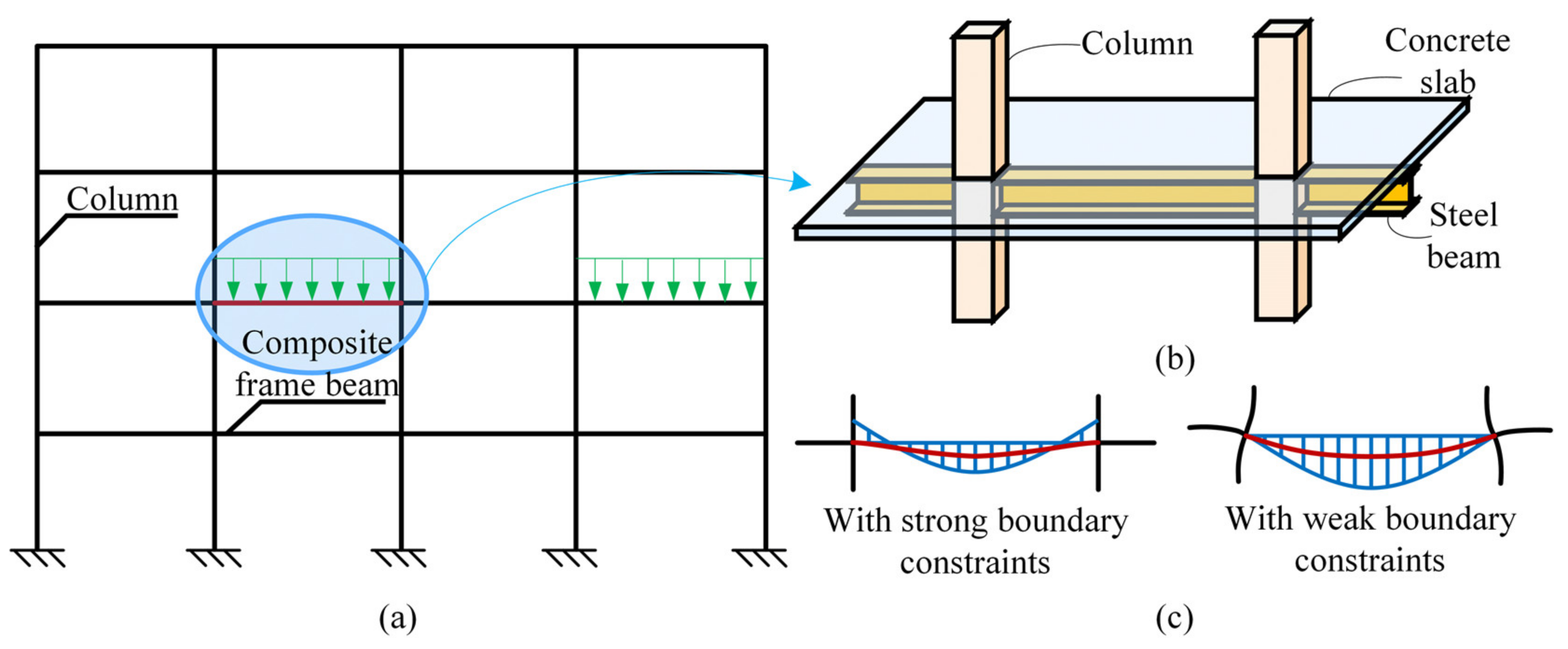
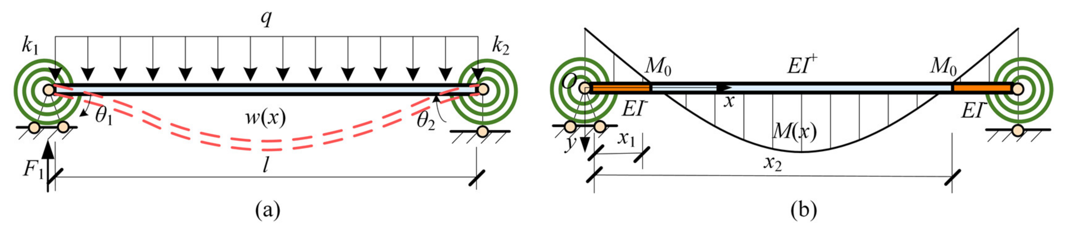
2. Theoretical Analysis

After the concrete slab cracking in the negative moment area, the effective flexural stiffness reduces and the composite beam performs an inelastic deformation. To discuss the inelastic bending deformation of composite frame beams, a theoretical model is established for a composite beam subject to a uniformly distributed vertical load. As shown in Figure 2, the composite beam is divided into three segments with different section flexural stiffness depending on the cracking of its concrete slab. For the middle segment of the beam, the concrete slab remains intact under a positive moment, and the section stiffness is defined as the normal value (EI⁺). However, the segments at the two ends of the beam suffer cracking in the concrete slab, and hence, the reduced section stiffness (EI⁻) is chosen. The spring constraint boundaries are also included in the proposed model to simulate in detail the rotation constraint imposed by the adjacent beams and columns in the frame structural system. As the full shear connection is assumed for all composite beams discussed in this study, the slip effect at the steel–concrete interfaces is neglected in the theoretical model as well as in the numerical model discussed in the following sections. This simplified treatment in modelling is validated to be reasonable by previous studies [3,32], especially when considering the slip constraint provided by the beam–column joints.

First, the internal force distribution of the composite beam is derived by the theoretical model. The reaction force at the left support is obtained from the equilibrium condition as

$$F_1=\frac{1}{2}ql+ \left(k_1{\theta }_1+k_2{\theta }_2\right)/l,$$

(2)

where q is the uniformly distributed vertical load applied on the composite beam; l is the length of the beam span; k₁ and k₂ represent the rotation restraint stiffness of the spring boundaries at the left and right ends of the beam, respectively; and θ₁ and θ₂ are the rotation angles at the two ends of the composite beam under the vertical load, respectively.

The moment distribution, M(x), of the composite beam can be expressed by the following equation:

$$M\left(x\right)=F_{1}x-k_1{\theta }_1-\frac{1}{2}q{x}^2,$$

(3)

where x is the distance of the calculated point to the left end support.

Based on the theory of material mechanics, the bending moment and vertical deflection of the composite beam satisfy the following relationship:

$$E{I}_i\frac{d^2{w}_i\left(x\right)}{d{x}^2}=-M\left(x\right),$$

(4)

where subscript i denotes the three segments of the composite beam, which are numbered from left to right as 1, 2, and 3, respectively; w_i(x) represents the distribution of the vertical deflection for the corresponding beam segment; and EI_i is the bending stiffness of the ith beam segment, being EI⁻ or EI⁺ depending on the segment. The contribution of reinforced steel rebars in the concrete slab is assumed to be negligible [3], and is thereby ignored in the calculation of EI⁻ and EI⁺.

The rotation angle distribution of the composite beam can be derived by integrating Equation (4) as follows:

$$E{I}_i{\theta }_i\left(x\right)=-\int M\left(x\right)dx=-\frac{1}{2}{F}_1{x}^2+k_1{\theta }_{1}x+\frac{1}{6}q{x}^3+C_{1i}$$

(5)

where θ_i(x) is the rotation angle distribution function of the corresponding beam segment; and C_1i is the integration constant, which is determined by the boundary conditions of the composite beam.

The distribution function of the vertical deflection can be further derived by integrating Equation (5) as follows:

$$E{I}_i{w}_i\left(x\right)=\int {\theta }_i\left(x\right)dx=-\frac{1}{6}{F}_1{x}^3+\frac{1}{2}{k}_1{\theta }_1{x}^2+\frac{1}{24}q{x}^4+C_{1i}x+C_{2i},$$

(6)

where C_2i is the integration constant, which is determined by the boundary conditions of the composite beam.

The boundary conditions of the composite beam in the frame structural system are as follows:

$$\left\{\begin{array}{c}M\left(x_1\right)=M\left(x_2\right)=M_0\\ {\theta }_1\left(0\right)={\theta }_1\\ {\theta }_3\left(l\right)={\theta }_2\\ w_1\left(0\right)=0\\ w_3\left(l\right)=0\\ {\theta }_1\left(x_1\right)={\theta }_2\left(x_1\right)\\ {\theta }_2\left(x_2\right)={\theta }_3\left(x_2\right)\\ w_1\left(x_1\right)=w_2\left(x_1\right)\\ w_2\left(x_2\right)=w_3\left(x_2\right)\end{array}\right. ,$$

(7)

where x₁ and x₂ represent the coordinates positions where the bending moments reach the value of cracking moment M₀ on the left and right sides of the composite beam, respectively.

Using the first boundary condition function expressed in Equation (7), the rotation angles at the beam ends—θ₁ and θ₂—can be expressed as follows:

$$\left\{\begin{array}{c}{\theta }_1=\frac{-q{x}_1{x}_2+2M_0}{2k_1}\\ {\theta }_2=\frac{-l^{2}q+lq{x}_1+lq{x}_2-q{x}_1{x}_2+2M_0}{2k_2}\end{array}\right. .$$

(8)

By substituting Equation (7) into Equations (5) and (6), all the integration constants (C_1i and C_2i, i = 1, 2, 3) can be eliminated, and thus, a non-linear equation system of x₁ and x₂ is obtained.

$$\left\{\begin{array}{c}\hfill k_2\left[6{EI}^{-}{I}^{+}q{x}_1{x}_2+I^{-}{k}_{1}q{(x}_1^3-3x_1^2{x}_2)+I^{+}{k}_{1}q(-x_1^3+3x_1^2{x}_2)+{12M}_0(-{EI}^{-}{I}^{+}+I^{-}{k}_1{x}_1-I^{+}{k}_1{x}_1)\right]\hfill \\ =k_1\left[\begin{array}{c}6{EI}^{-}{I}^{+}q\left(l-x_1\right)\left(x_2-l\right)+I^{-}{k}_{2}q{(x}_2^3-3x_1{x}_2^2)+I^{+}{k}_{2}q(-x_2^3+3x_1{x}_2^2-6l{x}_1{x}_2+3l^2\left(x_1+x_2\right)-2l^3)+\\ 12M_0({EI}^{-}{I}^{+}+I^{-}{k}_2{x}_2+I^{-}{k}_{2}l-I^{+}{k}_2{x}_2)\end{array}\right]\hfill \\ \hfill \hfill \\ \hfill k_2{x}_1^2\left(I^{-}q{x}_1^2-2I^{-}q{x}_1{x}_2-I^{+}q{x}_1^2+2I^{+}q{x}_1{x}_2+12I^{-}{M}_0-12I^{+}{M}_0\right)\hfill \\ ={12EI}^{-}{I}^{+}lq\left(l-x_1\right)\left(x_2-l\right)+I^{-}{k}_{2}q\left(x_2^4-2x_1{x}_2^3\right)+I^{+}{k}_{2}q\left(-x_2^4+2x_1{x}_2^3-6l^2{x}_1{x}_2+4l^3\left(x_1+x_2\right)-3l^4\right)+\hfill \\ 12M_0\left(2{EI}^{-}{I}^{+}l+I^{-}{k}_2{x}_2^2+I^{+}{k}_2{l}^2-I^{+}{k}_2{x}_2^2\right)\end{array}\right.$$

(9)

The non-linear system of equations can be solved using the Levenberg–Marquardt method; thus, all the parameters in Equation (9) can be determined by the given boundary conditions in practical cases. When the values of x₁ and x₂ are determined, the vertical deflection distribution as well as the equivalent flexural stiffness can be calculated by the following steps:

• x₁ and x₂ are substituted into Equation (7), and the rotation angles at the beam ends (θ₁ and θ₂) are solved;
• θ₁ and θ₂ are substituted into Equations (2) and (3) to solve the bending moment distribution function, M(x);
• M(x) is integrated using Equations (5) and (6), and the boundary condition functions (Equation (7)) are used to determine the integration constants (C_1i and C_2i, _i = 1, 2, 3). Therefore, the vertical deflection distributions of each beam segment (wi(x)) and the entire composite beam (w(x)) can be obtained.

3. Parameter Analysis

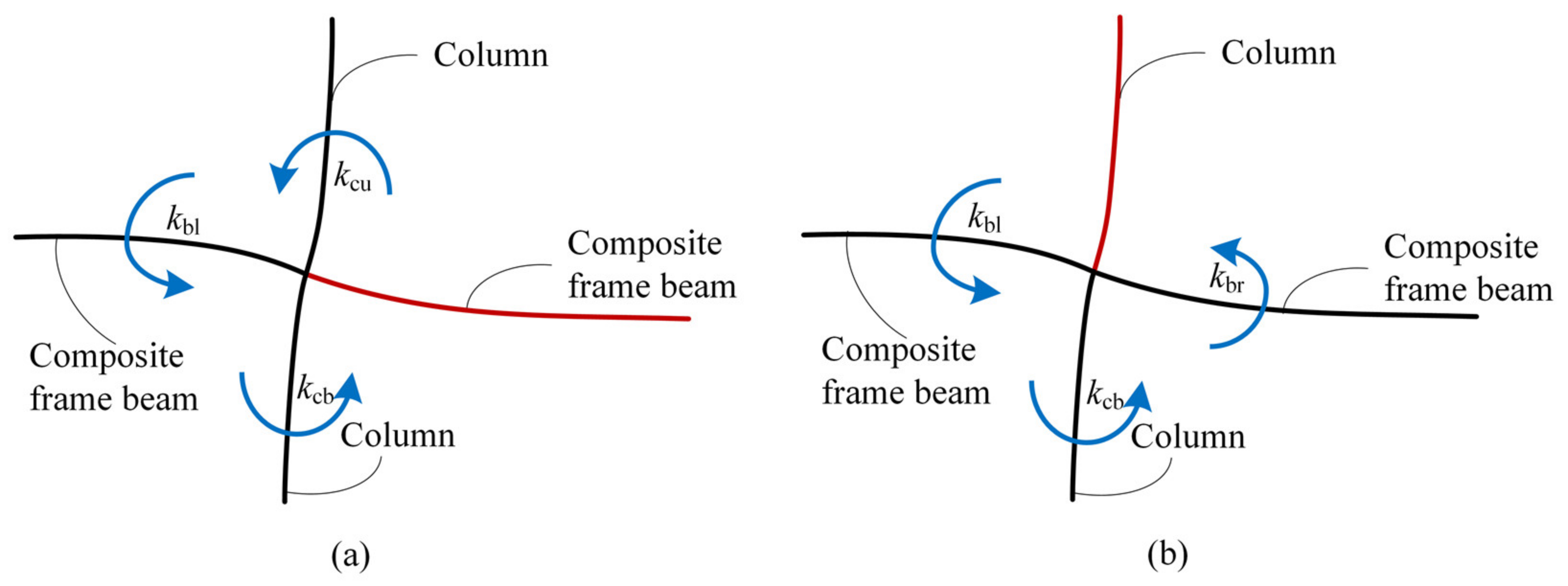
3.1. Rotation Constraints at Beam Ends

For a composite beam in a frame structural system, the rotation constraints at the beam ends are closely related to the surrounding beams and columns connected to it. In the theoretical model of the composite beam established above, the rotation constraints at the beam ends are simulated by spring constraint boundaries. To accurately evaluate the restraint stiffness at the beam ends, an equal-span composite frame structural system was selected to study the calculation method of parameter k_i (i = 1, 2).

For the planar beam–column joint shown in Figure 3, the rotation restraint stiffness at the beam end (k_b) and column end (k_c) can be calculated using Equation (10):

$$\left\{\begin{array}{c}{k}_{\mathrm{b}}=k_{\mathrm{cu}}+k_{\mathrm{bl}}+k_{\mathrm{cb}}\\ k_{\mathrm{c}}=k_{\mathrm{bl}}+k_{\mathrm{cb}}+k_{\mathrm{br}}\end{array}\right. ,$$

(10)

where k_cu, k_bl, k_cb, and k_br represent the rotation restraint stiffness provided by the surrounding beams and columns.

According to the mechanical principle of frame structure systems, the rotation restraint stiffness provided by a structural member to its adjacent members can be defined as a multiple of its linear stiffness:

$$k=ci=c\frac{EI}{l} ,$$

(11)

where c is the coefficient determined by the constraint condition at the other end; i is the linear stiffness of the member; EI is the flexural stiffness of the member; and l is the length of the member.

To simplify the calculation, all the beams and columns are assumed to have the same linear stiffness, i.e., k_cu = k_cb and k_bl = k_br. Thus, in the equal-span frame structural system, the rotation restraint stiffness at the ends of any beam or column member are the same, except for the case in which the beam or column member is located in the side span or top story. Thus, Equation (10) can be rewritten as Equation (12):

$$\left\{\begin{array}{c}{k}_b=c_1{i}_b+2c_2{i}_c\\ k_c=2c_1{i}_b+c_2{i}_c\end{array}\right. ,$$

(12)

where i_b and i_c are the linear stiffness of an adjacent beam and column, respectively, and c₁ and c₂ are the undetermined parameters that need to be calibrated by constraint stiffness k_b and k_c.

For a certain frame structural system with the given values of i_b and i_c, the values of c₁ and c₂ can be calculated by iteration. The calculation results indicate that the values of c₁ and c₂ are mainly related to the linear stiffness ratio of the beam and column (δ), as illustrated in Figure 4. In general, the value of δ varies from 0.1 to 5 and remains not greater than 1 for a composite frame structural system [28]. Within this parameter range, typically c₁ decreases with the increase in δ, whereas c₂ increases. However, it is noted from the figure that the values of c₁ and c₂ vary very little with δ in the given interval. Therefore, the average values of c₁ and c₂ (c₁ = 3.85, c₂ = 3.60) are used in Equation (12) and, thus, the rotation restraint stiffness at the composite beam ends can be approximately calculated using Equation (13):

$$k_i=3.85n{i}_b+3.60m{i}_c,$$

(13)

where n and m are, respectively, the numbers of beams and columns connected to the investigated composite beam.

Based on the displacement method in structural mechanics, the rotation constraint provided by a fixed supported beam to a far end is four times the linear stiffness of the member, whereas that by a hinged supported beam is thrice the linear stiffness. As the real boundary condition of a composite frame beam is between those of perfect fixed and hinged supports, the range of the rotation constraint coefficient should be from 3 to 4. This is consistent with the theoretical analysis of coefficients i_b and i_c, as previously discussed.

3.2. Identification of Critical Parameters

Using the theoretical model described in Section 2, an extensive parametric analysis was first conducted for the composite beam with equal rotation constraints at both ends, i.e., for the case of k₁ = k₂ (the unequal constraint case will be discussed in a subsequent section). The vertical deflection of the composite beam was proved to be primarily related to only three key parameters: (1) the linear stiffness of the composite beam before the concrete slab cracking (denoted as i⁺ = EI⁺/l); (2) the linear stiffness of the composite beam after the concrete slab cracking (denoted as i⁺ = EI⁺/l); and (3) the rotation constraint stiffness of the composite beam at both ends (denoted as k = k₁ = k₂). In addition, it was observed that, when these three factors change proportionally, i.e., increase or decrease simultaneously by the same multiple, the structural responses—vertical deflection, internal force, and equivalent flexural stiffness—of the concerned composite frame beam remained invariant. Therefore, two dimensionless parameters were identified as the dominant factors for the vertical deformation of composite beams. These are (1) the ratio of the rotation restraint stiffness and the linear stiffness of the composite beam after the concrete slab cracking (denoted as K = k/i⁻), and (2) the ratio of the linear stiffness of the composite beam before and after the concrete slab cracking (denoted as α = i⁺/i⁻).

To facilitate the detailed parameter analysis of the equivalent flexural stiffness of composite beams, the regular ranges of critical parameters K and α were determined based on the engineering practice. Parameter K represents the effect of the rotation constraints at the beam ends on the calculation of the equivalent flexural stiffness. This is discussed for two scenarios: common frame structures designed with equal-span arrangements and composite beams designed with large spans and heavy loads. For the case of common frame structures, the linear stiffness ratio of the composite beam and the column should range from 0.2 to 1, and thus, the range of parameter K was calculated to be 10–40 using Equation (13). For the case of composite beams designed with large spans and heavy loads, the range of parameter K was 4–10 based on relevant practical engineering examples [27].

Parameter α reflects the effect of the concrete slab cracking on the equivalent flexural stiffness of a composite beam, and it is also referred to as the stiffness amplification coefficient in structure design codes. According to the JGJ 138-2016 Chinese Code for Design of Composite Structure [33], the stiffness amplification coefficient, α, is calculated using Equation (14),

$$\alpha =\frac{2.2}{{(I_s/I_c)}^{0.3}-0.5}+1,$$

(14)

where I_c is the equivalent moment of inertia of the concrete slab section and I_s is the moment of inertia for a pure steel beam section.

Nie and co-workers [34,35] have completed numerous numerical studies on composite beams that considered the cracking effect of the concrete slab. Based on their analysis results, the value of parameter α is found to range from 1.1 to 7, which covers most engineering application cases of composite beams.

3.3. Consideration of Unequal Rotation Constraints at Beam Ends

For the case in which the rotation restraint stiffness at the left and right ends of a composite beam are unequal, the rotation constraints at both the need to be calculated independently. Two additional variables—total restraint stiffness (k_tot) and distribution coefficient (s)—are introduced to express the rotation restraint stiffness at the left and right ends of the composite beam as follows:

$$k_1=s{k}_{tot},$$

(15)

$$k_2=\left(1-s\right)k_{tot}.$$

(16)

Generally, the values of s range from 0.3 to 0.7 in engineering practices. When variable s = 0.5, the constraint stiffness at both the beam ends are the same, and, when it deviates from 0.5, the difference between them increases. By keeping parameters α and k_tot constant, the theoretical calculation results of the equivalent flexural stiffness of the composite beam are obtained, as shown in Figure 5. In the figure, the vertical coordinate axis represents the stiffness ratio of the composite beam to the steel beam, EI_eq/EI⁻, and the horizontal coordinate axis represents the variation in s.

This indicates that, when parameter k_tot is relatively small, EI_eq/EI⁻ decreases as variable s deviates from 0.5. Conversely, when variable k_tot is relatively large, EI_eq/ EI⁻ increases when variable s deviates from 0.5. Compared with the case when variable s = 0.5, the fluctuation range of EI_eq/EI⁻ does not exceed 3%. Therefore, the case in which the rotation restraint stiffness values are unequal at the two beam ends can be simplified as the equal rotation constraint case using an average value of the rotation restraint stiffness calculated by

$$k=\left(k_1+k_2\right)/2$$

(17)

3.4. Length of the Negative Moment Region

The length of the negative moment region is an important indicator in the design of composite frame beams. As shown in Figure 6, the length of the negative moment region is closely related to critical parameters K and α. Generally, the length of the negative moment region increases with the increase in parameter K. When parameter K, indicating the constraint stiffness at the ends of the composite beam, is zero, the frame beam degenerates to a simply supported beam, and thus, there is no negative moment region in the composite beam. As parameter K increases from 0 to 10, the length of the negative moment region increases rapidly, whereas when K exceeds 10, it keeps increasing, but at a relatively lower rate.

As discussed in Section 3.2, parameter K in the range of 0 to 10 represents composite beams designed with large spans and heavy loading conditions. In this case, the length of the negative moment region is sensitive to the constraint stiffness at the beam ends; thus, parameter K significantly affects the cracking of the concrete slab and the flexural stiffness distribution of the composite beam. However, in the traditional method for evaluating the effective flexural stiffness of a composite beam, the length of the negative moment region is generally taken as a constant without considering the boundary conditions. For example, GB 50017-2017 [28] and Eurocode 4 [29] define the negative moment regions as the segments with a 15% length of the span at both the beam ends and assign EI⁻ as the section flexural stiffness of the negative moment segments. The horizontal line representing the ratio of the length of the negative moment region to the beam span at 15% is also plotted in Figure 6. It indicates that a fixed value of 0.15 overestimates the length of the negative moment region, and overstating the cracking effect of the concrete slab results in a relatively smaller calculated value of the flexural stiffness of the composite beam.

When parameter K is fixed, the length of the negative moment region decreases with the increase in parameter α, i.e., the ratio of the linear stiffness of the composite beam before and after the concrete slab cracking. This is because, for a composite beam with a large sectional flexural stiffness in the non-cracked area, a large proportion of the internal force is shared by the positive moment region, and consequently, the cracking area, i.e., the length of the negative moment region, decreases.

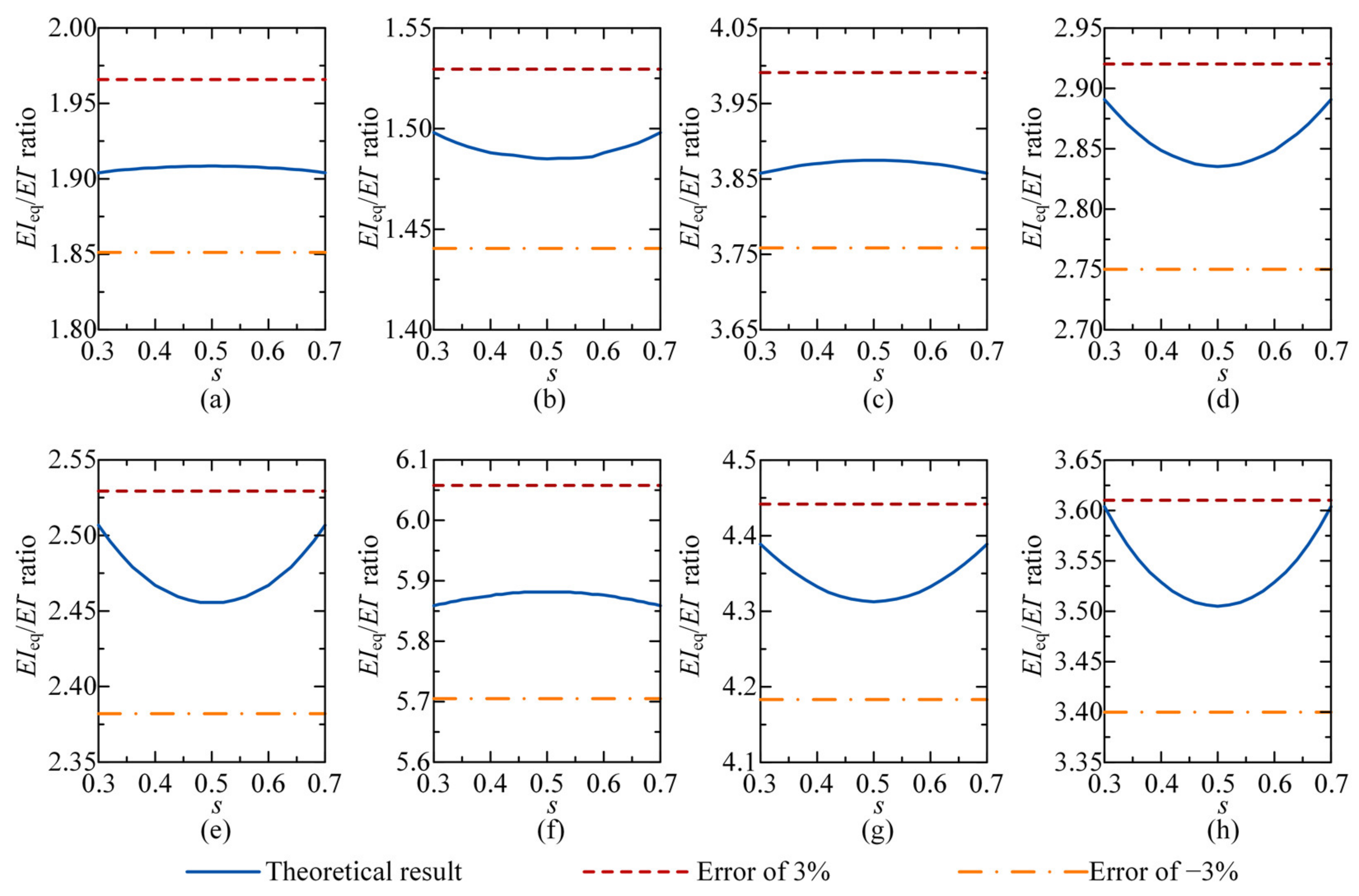
3.5. Equivalent Flexural Stiffness

For the convenience of structural design in engineering applications, an equivalent flexural stiffness represented by the weighted average of EI⁺ and EI⁻ is frequently used to evaluate the integral stiffness of a composite beam. The weight factor of the equivalent stiffness—parameter β in Equation (1)—can be calculated using the theoretical model presented in Section 2. The relationship between the weight factor and the rotational constraint stiffness (described by parameters K and α) is presented in Figure 7.

It can be seen that the computed value of β increases as parameter K increases, which indicates that a strong rotational constraint results in a small equivalent flexural stiffness. In addition, factor β initially increases rapidly when K is relatively small and subsequently changes gradually, approaching saturation. When parameter K is fixed, weight factor β increases as parameter α reduces, and the difference in the equivalent flexural stiffness is larger when K ranges from 10 to 20. In Figure 7, the calculated results of weight factor β are also compared with the recommended values of ANSI/AISC and Liew et al. It can be concluded that the fixed value of weight factor β cannot accurately describe the equivalent flexural stiffness of the composite beam because the effects of the boundary rotation constraints and the concrete slab cracking are not elaborately considered in most cases. In particular, for the composite beams designed with a large span and heavy loading, the rotation constraints at the beam ends are relatively weak and parameter K is small (e.g., 4–10) [27]. Fixed weight factor β, suggested by the previously mentioned studies, significantly underestimate the integral rigidity of the composite beam. For the commonly used frame structural system arranged with equal spans, parameter K varies within the values of 10–40 and parameter α is approximately 0.4. In this case, the recommended value of β provided in ANSI/AISC can reasonably describe the deformation mechanism and flexural stiffness of the composite beams. In comparison, the value of 0.6 suggested by Liew et al. leads to a remarkable difference from the theoretical results of β for both the large- and common-span beams.

Based on the parameter analysis, as prescribed, the rotational constraint condition is proved to have the dominant effect on the equivalent flexural stiffness of the composite beam. To consider the critical parameters of the rotational constraint—K and α—in evaluating the equivalent flexural stiffness, a simplified formula for calculating weight factor β is proposed by curve fitting, as expressed in Equation (18):

$$\beta =\frac{\left(0.02\alpha +0.49\right)K^{1.9}}{K^{1.9}+5.7{\alpha }^2+21.7\alpha +35.6} .$$

(18)

In Figure 7, the change in weight factor β calculated using Equation (18) is represented by solid lines. It can be seen that the calculated results of weight factor β agree well with those obtained from the theoretical model. Taking parameter K = 0 as an example, coefficient β is calculated to be 0 using Equation (18), and the equivalent flexural stiffness is EI⁺, which is in agreement with the theoretical results of a simply supported beam without the cracking effect. In addition, when parameter K approaches infinity, the limit of β is 0.02α + 0.49 and corresponds to the stiffness amplification coefficient, which is also in good agreement with the theoretical tendency of composite beams with a fixed support boundary.

4. Validation

To validate the accuracy of the proposed formula for evaluating the equivalent flexural stiffness of a composite frame beam, the calculated results were compared with those obtained from other design formulas as well as the simulation results of refined FE models.

4.1. Comparison with Existing Design Formulas

First, for conducting a parameter analysis, numerous design cases were selected from practical engineering. As shown in Figure 8, the analysed examples consisted of 180 composite beams with different cross-sections, in which the span length, L, ranges from 6 to 20 m. The effective slab width was calculated using the stiffness amplification coefficient, α, and the slab thickness ranged from 100 to 150 mm. The span-to-steel beam height ratio, L/h_s, ranged from 15 to 25, and the steel beam flange width to height ratio, b_f/h_s, ranged from 0.4 to 1.0. In addition, the steel beam flange thickness, t_f, and the web thickness, t_w, were also designed to satisfy the requirement of a compact section.

Subsequently, the analysed cases were divided into two groups based on the constraint boundary at the beam ends. In one group, parameter K ranged from 4 to 10, which represents the composite beams designed with large spans and heavy loads. In the other group, it ranged from 12 to 36, which represents the common composite frame beams arranged with equal spans. The calculated results of the proposed formula in this paper were compared with those obtained from the existing method, including the recommended methods of ANSI/AISC, Eurocode 8 [36], and Liew et al., as shown in Figure 9. Note that the related regulations in ANSI/AISC and Eurocode 8 are similar; thus, the results calculated by both methods are plotted as one. Compared with the theoretical methods of the equivalent flexural stiffness calculation, the formula proposed in this paper had a margin of error of less than 1%. In comparison, the average errors of the methods suggested by ANSI/AISC and Liew et al. were more than 10%, which is because of ignoring the constraint boundary condition at the beam ends.

4.2. Comparison with FE Analysis of Frame Structures

To consider the bearing mechanism of a composite beam in a frame structural system, the equivalent flexural stiffness calculated by the proposed formula was further validated by conducting an FE analysis of the entire process deformation of a frame structure. The numerical model was built based on a four-story and five-span plane frame, whose detailed design parameters are provided in Figure 10. As the main variable parameter, the spans of the composite beams adopted the values of 6, 9.5, 13, 16.5, and 20 m in the numerical examples. The effective width of the concrete slab in the composite beams was calculated using stiffness amplification coefficient α according to JGJ 138-2016 [33]. In addition, the sectional dimensions of the composite beams were divided into two groups. In one group, the concrete slab thickness, h_c, was 120 mm; the span-to-steel beam height ratio, L/h_s, was 20; and the steel bam flange width to height ratio, b_f/h_s, was 0.6. In the other group, the concrete slab thickness, h_c, was 150 mm; the span-to-steel beam height ratio, L/h_s, was 15, and the steel bam flange width to height ratio, b_f/h_s, is 1.0. For all the FE models, the parameters of steel beam flange thickness, t_f, and web thickness, t_w, were designed to satisfy the requirements of width-thickness ratios specified in GB 50017-2017. Based on the principle of ‘strong column–weak beam’ in structural design, the sectional sizes of the columns changed with the span of the frame beam, and the axial compression ratio of each column was set as approximately 0.4 to ensure that the columns do not yield before the beam achieves the ultimate limit state.

The FE models of the investigated frame structures were established using a modified fibre beam–column element proposed by the Tao and Nie teams [19], which was developed using the subroutine package, COMPONA-MARC, based on the general FE analysis software, MSC Marc. The accuracy of the modified fibre beam–column element in the non-linear analysis of composite frame systems was considerably validated [19,37]. Based on previous research on modelling strategies [32], the length of the fibre beam–column element was suggested to be as, approximately, the depth of the cross-section. In each cross-section of the beam elements, the concrete slab was divided into 5 × 5 fibres, i.e., 25 fibres in total; the beam flange was divided into 10 fibres; and the web plate was divided into 20 fibres. In each cross-section of the column elements, the flange and web plates were divided into 10 and 20 fibres, respectively. The constitutive law, suggested by Rüsch [38], was adopted for the uniaxial stress–strain skeleton curve of the concrete, and the constitutive relationship suggested by Esmaeilly et al. [39] was adopted for that of steel. The detailed parameters of the material constitutive model are shown in Figure 11.

A uniformly distributed load in the vertical direction was applied to the middle and side spans of the composite frame beams located in the first and fourth stories. The applied loads started at zero and continued to increase until the frame beams completely entered the plastic stage; thus, the entire evolution process of the deflection can be traced for the considered beams. The simulated load–deflection curves of some typical frame beams are presented in Figure 12a,b. By defining the point when the applied load achieves half of the ultimate stage as the normal service stage, the corresponding deflection at the middle of the span was compared with the results calculated by the proposed formula. The comparison suggests that the simplified formula expressed in Equation (18) can predict well the flexural stiffness of the composite beams in the service stage. For the 40 numerical examples of composite beams shown in Figure 12c, the vertical deformations calculated by the recommended formula agree well with the FE analysis results. The calculation errors of the investigated cases are all within 10%, which demonstrates that the proposed formula has good accuracy for evaluating the equivalent flexural stiffness of the composite beams.

5. Simplified Design Method

As discussed above, the rotation restraint stiffness at each beam end is the dominant factor in calculating the equivalent flexural stiffness of the composite frame beams. In the proposed formula, the rotation restraint stiffness of the frame beam is represented by parameter K, which needs to be determined in advance. However, the calculation of the rotation restraint stiffness—the value of parameter K—requires the calibration of the line stiffness for the adjacent structural members, such as the beams and columns connected to the considered frame beam. Thus, it is still complex to use the proposed formula to evaluate the equivalent flexural stiffness of a frame beam. To overcome this drawback in practical design, a simplified method for calculating the rotation constraints at the beam ends and a design formula for evaluating the vertical deflection of the frame beam are proposed in Section 5.1 and Section 5.2, respectively.

5.1. Simplified Method for Calculating Rotation Constraint Stiffness

The stiffness of the rotation constraints at the beam ends can be directly reflected by the bending moment distribution on the composite beam. As a rule, strong rotation constraints at the beam ends lead to large negative moment regions on the composite frame beam. Therefore, the rotation constraint stiffness can be represented by the length of the negative moment region by identifying the distribution trend of the internal force.

For a composite beam with a uniform flexural stiffness distribution and no concrete slab cracking, the reaction force at the beam support and the distributions of the bending moments, rotations, and vertical deflections on the composite beam can be derived using the theoretical model described in Section 2. These are expressed as follows:

$$F_1=\frac{1}{2}ql+\frac{k_1{\theta }_1+k_2{\theta }_2}{l},$$

(19)

$$M\left(x\right)=F_{1}x-k_1{\theta }_1-\frac{1}{2}q{x}^2,$$

(20)

$$E{I}^{+}\theta \left(x\right)=-\int M\left(x\right)dx=-\frac{1}{2}{F}_1{x}^2+k_1{\theta }_{1}x+\frac{1}{6}q{x}^3+C_1, \mathrm{and}$$

(21)

$$E{I}^{+}w\left(x\right)=\int \theta \left(x\right)dx=-\frac{1}{6}{F}_1{x}^3+\frac{1}{2}{k}_1{\theta }_1{x}^2+\frac{1}{24}q{x}^4+C_{1}x+C_2,$$

(22)

where the definitions of the notations are consistent with those specified in Section 2.

For frame beams with constant sectional stiffness, the boundary condition functions at the beam ends can be expressed as

$$\left\{\begin{array}{c}\theta \left(0\right)={\theta }_1\\ \theta \left(l\right)={\theta }_2\\ w\left(0\right)=0\\ \theta \left(l\right)=0\end{array}\right..$$

(23)

By substituting the boundary condition functions into Equations (21) and (22), θ₁ and θ₂ can be expressed as

$$\left\{\begin{array}{c}{\theta }_1=\frac{q{l}^3\left(6E{I}^{+}+k_{2}l\right)}{12\left[12{\left(E{I}^{+}\right)}^2+4E{I}^{+}\left(k_1+k_2\right)l+k_1{k}_2{l}^2\right]}\\ {\theta }_1=-\frac{q{l}^3\left(6E{I}^{+}+k_{1}l\right)}{12\left[12{\left(E{I}^{+}\right)}^2+4E{I}^{+}\left(k_1+k_2\right)l+k_1{k}_2{l}^2\right]}\end{array}.\right.$$

(24)

Subsequently, the internal force distribution functions listed in Equations (20)–(23) can be solved.

To build the relationship between the rotation constraint stiffness and the bending moment distribution, two additional parameters α_cr and l_cr are introduced to describe the length of a negative moment region, which are defined as follows:

$$\left\{\begin{array}{c}{\alpha }_{cr}=\frac{l_{cr1} + l_{cr2}}{l}\\ l_{cr}=l_{cr1}+l_{cr2}={\alpha }_{cr}l\end{array}\right.,$$

(25)

where l_cr1 and l_cr2 are the lengths of the negative moment regions located on the composite beam at the left and right ends, respectively; l_cr is the total length of the negative moment region; and l is the length of the composite beam span.

Based on the definitions of l_cr1 and l_cr2, the following relationship should be satisfied:

$$M\left(l_{cr1}\right)=M\left(l-l_{cr2}\right)=0$$

(26)

Thus, the rotation restraint stiffness can be expressed as

$$\left\{\begin{array}{c}{k}_1=\frac{12E{I}^{+}{l}_{cr1}\left(l-l_{cr2}\right)}{l\left(l^2-2l{l}_{cr2}-4l{l}_{cr1}+6l_{cr1}{l}_{cr2}\right)}\\ k_2=\frac{12E{I}^{+}\left(l-l_{cr1}\right)l_{cr2}}{l\left(l^2-2l{l}_{\mathrm{cr}1}-4l{l}_{\mathrm{cr}2}+6l_{cr1}{l}_{\mathrm{cr}2}\right)}\end{array}.\right.$$

(27)

If the rotation restraint stiffness at both the ends of the beam are equal (k₁ = k₂), the lengths of the negative moment regions at the beam ends are equal, and the following results can be obtained:

$$l_{cr1}=l_{cr2}=\frac{1}{2}{\alpha }_{cr}l,$$

(28)

$$k_1=k_2=\frac{6E{I}^{+}\left(2{\alpha }_{\mathrm{cr}}-{\alpha }_{\mathrm{cr}}{}^2\right)}{l\left(2-6{\alpha }_{\mathrm{cr}}+3{\alpha }_{\mathrm{cr}}{}^2\right)}.$$

(29)

For the case in which the rotation restraint stiffness at the two ends of the beam are unequal, the lengths of the negative moment regions at the beam ends are different. The unequal distribution of the negative moment regions is described by the total length of the negative moment regions (l_cr) and the distribution coefficient (s), as defined in Equation (30):

$$s=\frac{l_{cr1}}{l_{cr}}=1-\frac{l_{cr2}}{l_{cr}}.$$

(30)

Based on the theoretical model, the equivalent flexural stiffness (EI_eq) is calculated from the varied values of l_cr and s, and the results are presented in the normalized form of the stiffness ratio, EI_eq/EI⁻, as shown in Figure 13. It can be seen that, when distribution coefficient s deviates from 0.5, EI_eq/EI⁻ decreases. However, compared with the calculation results when s = 0.5, the fluctuation range of EI_eq/EI⁻ does not exceed 4% when s varies within 0.3–0.7, which covers the range of interest in practice engineering. Therefore, for the case in which the lengths of the negative moment regions are unequal at the two beam ends, i.e., $s\ne 0.5$, it is acceptable to simplify the calculation of the rotation restraint stiffness using the average value of l_cr1 and l_cr2.

5.2. Simplified Design Formula for Calculating Vertical Deflection

To utilize Equation (18) to calculate the vertical deflection of a composite beam, two critical parameters, i.e., K and α, need to be calibrated first. By substituting Equation (29) into the definition formula of K, the ratio of the rotation restraint stiffness and the linear stiffness of the composite beam after the concrete slab cracking can be easily obtained as

$$K=\frac{k}{i^{-}}=\frac{6\alpha \left(2{\alpha }_{\mathrm{cr}}-{\alpha }_{\mathrm{cr}}{}^2\right)}{\left(2-6{\alpha }_{\mathrm{cr}}+3{\alpha }_{\mathrm{cr}}{}^2\right)}.$$

(31)

Figure 14 illustrates the relationship between parameter K and negative moment region factor α_cr for different values of parameter α. Generally, when α is fixed, parameter K increases as the negative moment region increases. Note that when α_cr = 0, the composite frame beam degenerates to a simply supported beam and parameter K = zero. When α_cr is close to its theoretical maximum value of $1-\sqrt{3}/3$, parameter K approaches infinity. For the case when α_cr is fixed, parameter K increases as the stiffness amplification coefficient α becomes larger, which indicates that a large flexure stiffness of the composite beam leads to strong rotation constraints at the beam ends.

In practical design, critical parameter K can be calculated using coefficients α and α_cr in Equation (31). The weight factor of the equivalent stiffness, β, can also be calculated using this simplified method, and the relationship between parameters β and α_cr is presented in Figure 15.

To facilitate the utilization of this simplified method, a vertical deflection correction factor α_Δ is introduced and defined as follows:

$${\alpha }_{\mathsf{\Delta }}=\frac{{\mathsf{\Delta }}_{\mathrm{co}}}{\mathsf{\Delta }}$$

(32)

where Δ_co is the vertical deflection of the composite frame beam considering the effect of the concrete slab cracking and Δ is the vertical deflection of the composite beam neglecting the effect of the concrete slab cracking.

Based on the relationship between the flexural stiffness and the vertical deflection of the composite beam during the elastic stage, the definition of the vertical deflection correction factor, α_Δ, can be rewritten as

$${\alpha }_{\Delta }=\frac{E{I}^{+}}{E{I}_{\mathrm{eq}}}=\frac{\alpha }{\beta +\left(1-\beta \right)\alpha }$$

(33)

For composite frame beams with different cross-section properties and rotation constraints, the theoretical value of α_Δ can be calculated using Equation (33). Figure 16 illustrates the relationship of α_Δ with the negative moment region factor, α_cr, for different values of the stiffness amplification coefficient, α. As expressed in Equation (33), α_Δ is determined using the equivalent flexural stiffness weight coefficient, β, and the stiffness amplification coefficient, α, where β is determined by critical parameters K and α. In addition, if the elastic analysis results of the internal force of a frame structure are available, parameter K can be further expressed using α and α_cr. Therefore, it is reasonable to use the stiffness amplification coefficient, α, and the negative moment region factor, α_cr, as independent variables when determining the vertical deflection correction factor, α_Δ. Based on the theoretical analysis results of α_Δ shown in Figure 16, a piecewise function is proposed as the simplified design formula for calculating the vertical deflection correction factor, α_Δ:

$${\alpha }_{\Delta }=\left\{\begin{array}{c}1,\hspace{0.33em}\hspace{0.33em}\hspace{0.33em}\hspace{0.33em}{\alpha }_{cr}\le 0.1\\ \frac{\left({\xi }_1-1\right){\alpha }_{cr}+\left(0.25-0.1{\xi }_1\right)}{0.15},\hspace{0.33em}\hspace{0.33em}\hspace{0.33em}\hspace{0.33em}0.1<{\alpha }_{cr}\le 0.25\\ \frac{\left({\xi }_2-{\xi }_1\right){\alpha }_{cr}+\left(0.43{\xi }_1-0.25{\xi }_2\right)}{0.18},\hspace{0.33em}\hspace{0.33em}\hspace{0.33em}\hspace{0.33em}{\alpha }_{cr}>0.25\end{array}\right.,$$

(34)

where ξ₁ and ξ₂ are the calculated values of the vertical deflection correction factor when α_cr = 0.25 and 0.43, respectively, which can be calibrated by the following equations:

$${\xi }_1=0.06\alpha +0.96, {\alpha }_{cr}=0.25,$$

(35)

$${\xi }_2=-0.03{\alpha }^2+0.466\alpha +0.61, {\alpha }_{cr}=0.43$$

(36)

As shown in Figure 16, there is a good agreement between the calculation results of the simplified design formula and the theoretical model. It is demonstrated that, by elaborately considering the rotation constraints at the beam ends and the cracking effect in the concrete slab, the proposed design formula can accurately describe the equivalent flexural stiffness of the composite beams. The vertical deflection correction factor, α_Δ, is observed to increase with the increase in the negative moment region factor, α_cr, or the stiffness amplification coefficient, α, which is consistent with the theoretical analysis results as previously discussed. For the particular case of α_cr = 0, correction factor α_Δ = 1, as calculated using Equation (34), indicates that the simply supported composite beam does not need to adjust the calculated vertical deflection of the elastic analysis.

In summary, using the proposed design formula, as described in the following steps, the vertical deflection of composite frame beams can be easily calculated:

• Based on the elastic analysis results of a structural design software, the lengths of the negative moment regions, l_cr1 and l_cr2, can be obtained from the internal force distributions. Subsequently, the negative moment region factor, α_cr, can be calculated using Equation (25);
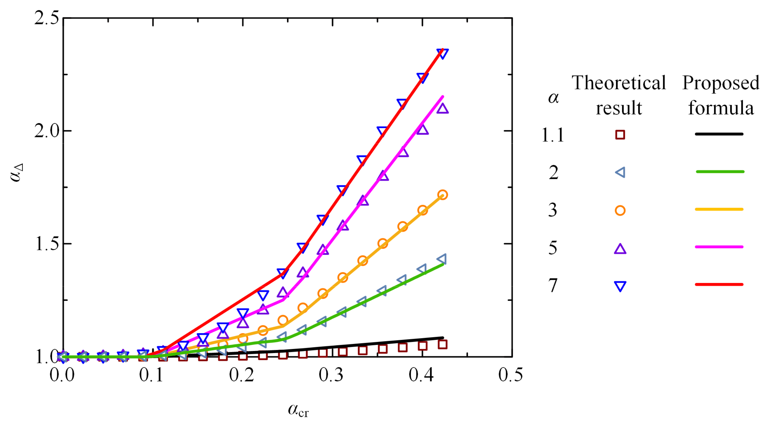
• By substituting parameter α_cr and stiffness amplification coefficient α into Equation (34), the vertical deflection correction factor, α_Δ, can be obtained;
• Utilizing the deformation results of the elastic analysis, the design value of the vertical deflection of the composite frame beam is determined using the proposed formula in Equation (32).

6. Conclusions

Based on the concept of equivalent flexural stiffness, a simplified design method is proposed to calculate the vertical deflection of a composite frame beam. To identify the influence of the rotation restraint stiffness at the beam ends and the cracked section in the negative moment regions, a theoretical beam model is established. By conducting an extensive parameter analysis of different frame beams, a fitting formula for evaluating the equivalent flexural stiffness as well as a simplified design formula for calculating the vertical deflection are proposed. The main conclusions are summarized as follows:

• For a composite frame beam under uniform vertical loading, the rotation restraint stiffness at the two beam ends has a significant effect on its vertical deflection and internal force distribution, which should be elaborately considered when calculating its equivalent flexural stiffness;
• By considering the boundary constraint conditions at the beam ends, the proposed formula for calculating the equivalent flexural stiffness can reasonably describe the deformation mechanism of a composite frame beam, presenting a higher calculation accuracy than those of the recommended formulas in ANSI/AICS and by Liew et al.;
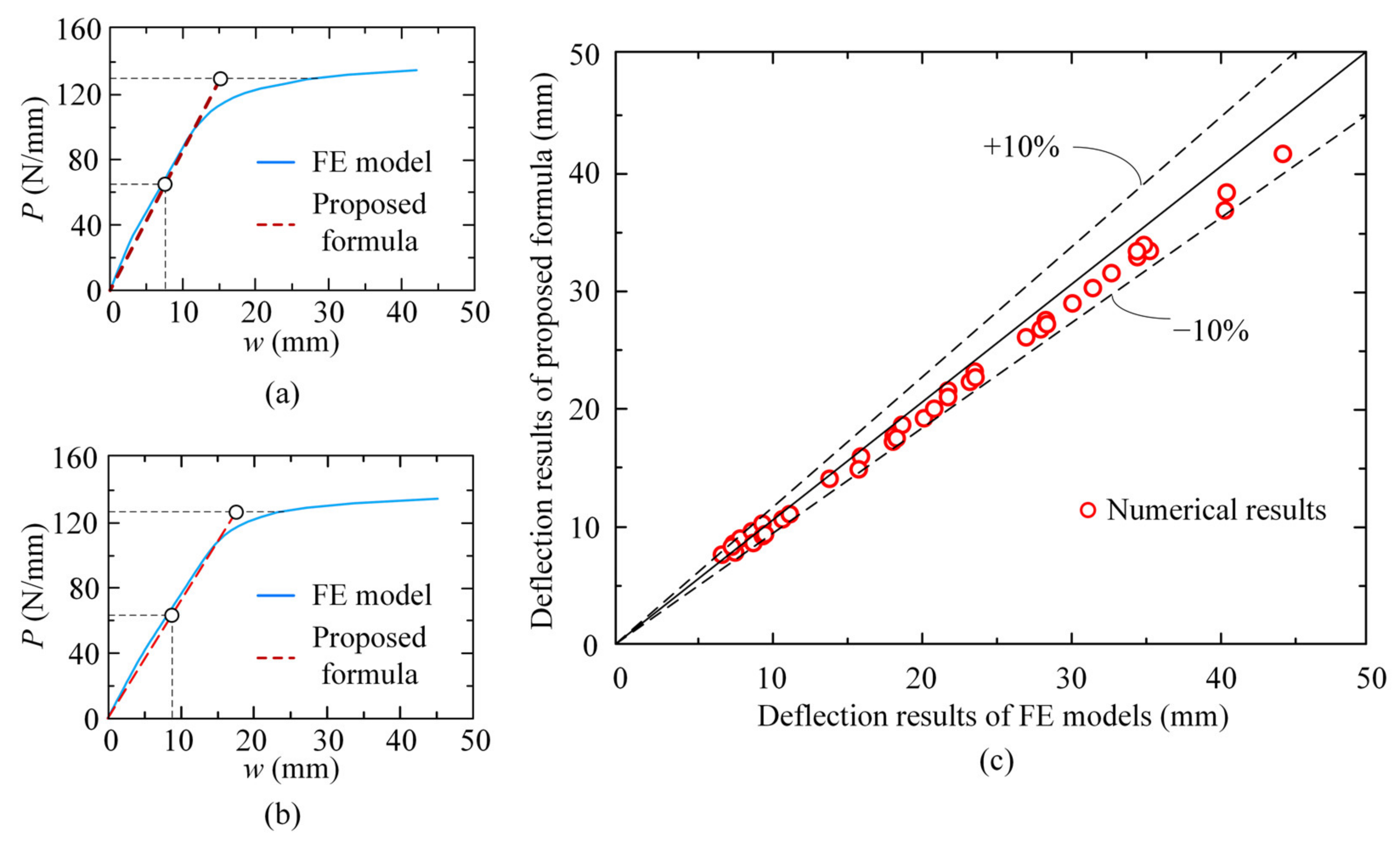
• By comparing with the non-linear FE analysis results of multiple entire frame structures, the accuracy and reliability of the proposed formula is further validated. The vertical deflections in the service stage calculated using the proposed formula agree well with those obtained from the entire process load–displacement curves in the FE analysis;
• Utilising the internal force distribution of a frame beam by elastic analysis, a simplified, but effective design method is proposed to calculate the vertical deflection. The design procedure is based on the deflection correction of the non-cracking analysis results, which is demonstrated to capture the influence of the complex boundary conditions and can be easily used in the practical design of composite frame beams.

References

1. Bursi, O.S.; Gramola, G. Behaviour of composite substructures with full and partial shear connection under quasi-static cyclic and pseudo-dynamic displacements. Mater. Struct. 2000, 33, 154–163. [Google Scholar] [CrossRef]
2. Udagawa, K.; Mimura, H. Behavior of composite beam frame by pseudodynamic testing. J. Struct. Eng. ASCE 1991, 117, 1317–1335. [Google Scholar] [CrossRef]
3. Zona, A.; Barbato, M.; Conte, J.P. Nonlinear seismic response analysis of steel–concrete composite frames. J. Struct. Eng. 2008, 134, 986–997. [Google Scholar] [CrossRef]
4. Nakashima, M.; Matsumiya, T.; Suita, K.; Zhou, F. Full-scale test of composite frame under large cyclic loading. J. Struct. Eng. 2007, 133, 297–304. [Google Scholar] [CrossRef]
5. Wang, Y.H.; Nie, J.G.; Cai, C.S. Numerical modeling on concrete structures and steel–concrete composite frame structures. Comp. Part B Eng. 2013, 51, 58–67. [Google Scholar] [CrossRef]
6. Ramnavas, M.P.; Patel, K.A.; Chaudhary, S.; Nagpal, A.K. Service load analysis of composite frames using cracked span length frame element. Eng. Struct. 2017, 132, 733–744. [Google Scholar] [CrossRef]
7. Akbas, S.D. Large deflection analysis of a fiber reinforced composite beam. Steel Compos. Struct. 2018, 27, 567–576. [Google Scholar] [CrossRef]
8. Chiorean, C.G.; Buru, S.M. Practical nonlinear inelastic analysis method of composite steel-concrete beams with partial composite action. Eng. Struct. 2017, 134, 74–106. [Google Scholar] [CrossRef]
9. Kirkland, B.; Uy, B. Behaviour and design of composite beams subjected to flexure and axial load. Steel Compos. Struct. 2015, 19, 615–633. [Google Scholar] [CrossRef]
10. Mirambell, E.; Bonilla, J.; Bezerra, L.M.; Clero, B. Numerical study on the deflections of steel-concrete composite beams with partial interaction. Steel Compos. Struct. 2021, 38, 67–78. [Google Scholar] [CrossRef]
11. Vasdravellis, G.; Uy, B. Shear strength and moment-shear interaction in steel-concrete composite beams. J. Struct. Eng. 2014, 140, 04014084. [Google Scholar] [CrossRef]
12. Kirkland, B.; Kim, P.; Uy, B.; Vasdravellis, G. Moment–shear–axial force interaction in composite beams. J. Constr. Steel. Res. 2015, 114, 66–76. [Google Scholar] [CrossRef]
13. Soto, A.G.; Caldentey, A.P.; Peiretti, H.C.; Benitez, J.C. Experimental behaviour of steel-concrete composite box girders subject bending, shear and torsion. Eng. Struct. 2020, 206, 110169. [Google Scholar] [CrossRef]
14. Newmark, N.M. Test and analysis of composite beams with incomplete interaction. Proc. Soc. Exp. Stress Anal. 1951, 9, 75–92. [Google Scholar]
15. Lawson, R.M.; Lam, D.; Aggelopoulos, E.S.; Nellinger, S. Serviceability performance of steel–concrete composite beams. Proc. Inst. Civil Eng. Struct. Build. 2017, 170, 98–114. [Google Scholar] [CrossRef] [Green Version]
16. Ding, F.X.; Liu, J.; Liu, X.M.; Guo, F.Q.; Jiang, L.Z. Flexural stiffness of steel-concrete composite beam under positive moment. Steel Compos. Struct. 2016, 20, 1369–1389. [Google Scholar] [CrossRef]
17. Liu, J.; Ding, F.X.; Liu, X.M.; Yu, Z.W. Study on flexural capacity of simply supported steel-concrete composite beam. Steel Compos. Struct. 2016, 21, 829–847. [Google Scholar] [CrossRef]
18. Liu, J.; Ding, F.X.; Liu, X.M.; Yu, Z.W.; Tan, Z.; Huang, J.W. Flexural Capacity of Steel-Concrete Composite Beams under Hogging Moment. Adv. Civ. Eng. 2019, 2019, 3453274. [Google Scholar] [CrossRef] [Green Version]
19. Tao, M.X.; Nie, J.G. Fiber beam-column model considering slab spatial composite effect for nonlinear analysis of composite frame systems. J. Struct. Eng. 2013, 140, 04013039. [Google Scholar] [CrossRef]
20. Zhang, Q.H.; Jia, D.L.; Bao, Y.; Dong, S.; Cheng, Z.Y.; Bu, Y.Z. Flexural behavior of steel–concrete composite beams considering interlayer slip. J. Struct. Eng. 2019, 145, 04019084. [Google Scholar] [CrossRef]
21. Lou, T.J.; Wu, S.S.; Karavasilis, T.L.; Chen, B. Long-term deflection prediction in steel-concrete composite beams. Steel Compos. Struct. 2021, 39, 21–33. [Google Scholar] [CrossRef]
22. Fragiacomo, M.; Amadio, C.; Macorini, L. Finite-element model for collapse and long-term analysis of steel–concrete composite beams. J. Struct. Eng. 2004, 130, 489–497. [Google Scholar] [CrossRef]
23. Wang, Y.H.; Yu, J.; Liu, J.P.; Zhou, B.X.; Chen, Y.F. Experimental study on assembled monolithic steel-prestressed concrete composite beam in negative moment. J. Constr. Steel. Res. 2020, 167, 105667. [Google Scholar] [CrossRef]
24. Shamass, R.; Cashell, K.A. Behaviour of composite beams made using high strength steel. Struct. 2017, 12, 88–101. [Google Scholar] [CrossRef]
25. Shi, Y.; Yang, K.D.; Guan, Y.; Yao, X.M.; Xu, L.; Zhang, H.B. The flexural behavior of cold-formed steel composite beams. Eng. Struct. 2020, 218, 110819. [Google Scholar] [CrossRef]
26. Yang, T.; Liu, S.Y.; Qin, B.X.; Liu, Y.Q. Experimental study on multi-bolt shear connectors of prefabricated steel-concrete composite beams. J. Constr. Steel. Res. 2020, 173, 106260. [Google Scholar] [CrossRef]
27. Nie, J.G.; Pan, W.H.; Tao, M.X.; Zhu, Y.Z. Experimental and numerical investigations of composite frames with innovative composite transfer beams. J. Struct. Eng. 2017, 143, 04017041. [Google Scholar] [CrossRef]
28. GB 50017-2017. Code for Design of Steel Structures; Ministry of Housing and Urban-Rural Development of the People’s Republic of China: Beijing, China, 2017. (In Chinese)
29. EN 1994-1-1:2004, Eurocode 4: Design of Composite Steel and Concrete Structures–Part 1-1: General Rules and Rules for Buildings; European Committee for Standardization: Brussels, Belgium, 2004.
30. ANSI/AISC 360-10, AISC Committee, Specification for Structural Steel Buildings; American Institute of Steel Construction: Chicago, IL, America, 2010.
31. Liew, J.Y.R.; Chen, H.; Shanmugam, N.E. Inelastic analysis of steel frames with composite beams. J. Struct. Eng. 2001, 127, 194–202. [Google Scholar] [CrossRef]
32. Nie, J.G.; Tao, M.X.; Cai, C.S.; Chen, G. Modeling and investigation of elasto-plastic behavior of steel–concrete composite frame systems. J. Constr. Steel Res. 2011, 67, 1973–1984. [Google Scholar] [CrossRef]
33. JGJ 138-2016, Code for Design of Composite Structures; Ministry of Housing and Urban-Rural Development of the People’s Republic of China: Beijing, China, 2016. (In Chinese)
34. Nie, J.G.; Tao, M.X. Slab spatial composite effect in composite frame systems. I: Effective width for ultimate loading capacity. Eng. Struct. 2012, 38, 185–199. [Google Scholar] [CrossRef]
35. Nie, J.G.; Tao, M.X. Slab spatial composite effect in composite frame systems. II: Equivalent stiffness and verifications. Eng. Struct. 2012, 38, 171–184. [Google Scholar] [CrossRef]
36. BS EN 1998-1:2004. Eurocode 8: Design of Structures for Earthquake Resistance–Part 1: General Rules, Seismic Actions and Rules for Buildings; European Committee for Standardization: Brussels, Belgium, 2004.
37. Tao, M.X.; Nie, J.G. Element mesh, section discretization and material hysteretic laws for fiber beam–column elements of composite structural members. Mater. Struct. 2015, 48, 2521–2544. [Google Scholar] [CrossRef]
38. Rusch, H. Researches toward a general flexural theory for structural concrete. J. Am. Concr. Inst. 1960, 57, 1–28. [Google Scholar]
39. Esmaeily, A.; Xiao, Y. Behavior of reinforced concrete columns under variable axial loads: Analysis. ACI Struct. J. 2005, 102, 736–744. [Google Scholar]
Figure 1. Bending mechanism of the composite frame beam in a structural system. ((a) Composite frame structural system; (b) Composite frame beam; (c) Deformation and bending moment diagram of composite frame beam).
Applsci 11 10305 g001
Figure 2. Theoretical model of the composite frame beam under uniform vertical loads. ((a) Boundary constraints and deformation; (b) Moment and section stiffness distribution).
Applsci 11 10305 g002
Figure 3. Composition of end rotation constraints stiffness of the beams and columns in the frame. ((a) Rotation constraints at beam ends; (b) Rotation constraints at column ends).
Applsci 11 10305 g003
Figure 4. Variation in c1 and c2 with beam-to-column line stiffness ratio. ((a) Relationship between c1 and δ; (b) Relationship between c2 and δ).
Applsci 11 10305 g004
Figure 5. Influence of end rotational constraint stiffness distribution on the equivalent flexural stiffness of the composite beam. ((a)α = 2, ktot = 10; (b) α = 2, ktot = 100; (c) α = 4, ktot = 10; (d) α = 4, ktot = 50; (e) α = 4, ktot = 100; (f) α = 6, ktot = 10; (g) α = 6, ktot = 50; (h) α = 6, ktot = 100).
Applsci 11 10305 g005
Figure 6. Variation in the length of the negative moment region with critical parameters K and α.
Applsci 11 10305 g006
Figure 7. Variation in the weight factor of equivalent stiffness with end rotational restraint stiffness.
Applsci 11 10305 g007
Figure 8. Numerical examples of the composite frame beam.
Applsci 11 10305 g008
Figure 9. Comparison of the equivalent flexural stiffness calculated by the formula proposed in this paper and other existing methods. ((a) Comparison of EIeq calculation results in large-span heavy-loading design conditions; (b) Comparison of EIeq calculation results in commonly arranged frame design conditions).
Applsci 11 10305 g009
Figure 10. Finite element model of the composite frame example.
Applsci 11 10305 g010
Figure 11. Skeleton curve of the stress–strain constitutive law used for steel and concrete. ((a) Stress−strain relation of steel; (b) Stress−strain relation of concrete).
Applsci 11 10305 g011
Figure 12. Comparison between the calculation results of the proposed formula and the FE analysis. ((a) Load−deflection curve of 6-m-span frame at middle span in 1st story; (b) Load−deflection curve of 6-m-span frame at side span in 4th story; (c) Comparison of deflection results between proposed formula and FE models).
Applsci 11 10305 g012
Figure 13. Effects of the unequal distribution of the negative moment regions on the equivalent flexural stiffness. ((a) α = 2, αcr = 0.2;(b) α = 2, αcr = 0.3;(c) α = 2, αcr = 0.4;(d) α = 4, αcr = 0.12; (e) α = 4, αcr = 0.25; (f) α = 4, αcr = 0.35; (g) α = 6, αcr = 0.1; (h) α = 6, αcr = 0.2; (i) α = 6, αcr = 0.32).
Applsci 11 10305 g013
Figure 14. Relationship between parameter K and negative moment region factor αcr.
Applsci 11 10305 g014
Figure 15. Variation in equivalent stiffness weight coefficient β with parameters α and αcr.
Applsci 11 10305 g015
Figure 16. Variation in vertical deflection correction factor αΔ with parameters α and αcr.
Applsci 11 10305 g016
Publisher’s Note: MDPI stays neutral with regard to jurisdictional claims in published maps and institutional affiliations.