User Satisfaction Survey on Public Transport by a New PAHP Based Model

Abstract

There is an obvious trade-off between information obtained from passenger surveys and cost and time investment. This paper offers a new approach for this problem and its detailed step-by-step procedure description. Parsimonious Analytic Hierarchy Process (PAHP) is a recently created methodology that combines the simplicity of direct evaluations with the consistency and reliability of the Analytic Hierarchy Process (AHP). In the paper, the first large sample survey of passenger satisfaction by a new, PAHP-based model and procedure is presented as a case study. Moreover, a comparison with an AHP survey on the same public transport system and the same pattern are demonstrated. Since the comparative analysis produced a strong correlation between AHP and PAHP outcomes, it can be stated that the new procedure is less time consuming and costly than the AHP, while possessing the same benefits, and thus, it is more trustworthy than satisfaction measured by direct evaluations. Consequently, our proposed model can be applied both in theoretical and practical cases. Theoretically, it solves the problem of avoiding the use of large pairwise comparison matrices, and practically, it is a useful support to public satisfaction surveys, especially in the transportation sector.

1. Introduction

Surveying the passengers has become an integrated part of transport policy in recent years. Collecting information on the motivation for travel, origins and destinations, and satisfaction with service elements or with transport service as a whole could all be objectives of these surveys. Two limitations restrict the process: budget and duration. The first determines the possible sample size; the latter one is a key factor for obtaining valid and quality responses [1]. However, conflicting objectives have to be considered for the decision makers of the transport policy. On one hand, results have to be representative, reflecting the preferences of the total community as much as possible, and from this perspective a large pattern and many respondents are required. On the other hand, responses should be detailed and suitable for and in-depth analysis, also be consistent and reliable; thus, long questionnaires and personal interviews are suggested. In practice, both requirements cannot be fulfilled simultaneously in many cases due to budget and duration limitations. Theory has discovered this conflict and models have emerged that endeavor to balance the complexity of the questionnaires (detailed surveys) and the validity and reliability of the responses (short, simple surveys).

This paper aims to contribute to the existing scientific literature by introducing a new, multi-level Parsimonious Analytic Hierarchy Process (PAHP) model which reduces survey duration significantly but still ensures validity of the responses by an in-built consistency check provided by an Analytic Hierarchy Process (AHP) phase.

The model has been tested in a real public transport development case, on a large sample (500 respondents), in a big Turkish city, Mersin. Previously, in the autumn of 2019, another survey was conducted on the same public bus transportation system by applying conventional AHP, with the same decision hierarchy; thus, the results of the recent and previous study are comparable.

The paper proposes a PAHP model which reduces survey duration significantly but still ensures validity of the responses by an in-built consistency check provided by an AHP phase.

The remaining of this paper includes an overview of public transport survey models, especially those that considered the reduction of respondent efforts. Further, since the parsimonious approach of AHP is new, it is introduced in detail, and then, the new multi-level created PAHP model is presented. Afterwards, the results of the case study are analyzed and compared to the previous, conventional AHP research results. Finally, conclusions are drawn not only for the specific case but also generally, with the objective that the created model might be applied to arbitrary public transport satisfaction surveys.

2. Literature Review

Passenger satisfaction refers to the passengers’ sense of either enjoyment or displeasure, which results from a comparison between function of the transport system and passenger’s expectations; however, investigating passenger satisfaction and perceived comfort related to public transportation has been in focus of many researchers since the 1970s, and the evolution of the applied models and questionnaires is palpable [2]. One direction of this evolution is involving more and more specified attributes characterizing the public transport service quality. The Quattro project (1999) applied merely seven attributes plus a K coefficient for determining the equivalent travel time as a synthetic performance measure in urban public transport [3], while [4] used 25 manifest and 10 latent variables to evaluate passenger satisfaction. Specifically, for measuring satisfaction for public bus transport, [5] created the Service Quality Index (SQI), integrating 13 attributes such as bus travel time, transport fare, general cleanliness on board, or seat availability on bus, while Duleba et al. [6] applied 24 factors designed in a three-level-hierarchy. Obviously, avoiding the application of too many factors is highly recommended because many attributes make the evaluation process long and complicated; however, too few variables might not be sufficient for the appropriate analysis of passenger satisfaction. Based on empirical evidence [7,8,9,10], the recommended number of attributes for characterizing passenger satisfaction for urban bus transport service is between 15 and 25.

Since a significant reduction of the examined factors of public transport service quality decreases the chance for complex analysis, the other possibility for creating a suitable questionnaire and reaching research goals with limited number of attributes is to apply a methodology capable of revealing sufficient information from the survey data. The requirement for the selected technique is, on one hand, to make the evaluations as light as possible (for gathering representative number of responses) and, on the other hand, to provide the opportunity for proper analysis applying the given number of attributes.

There has been a wide range of techniques applied for passenger satisfaction surveys. One of the earliest is the Stated Preference approach [11,12], in which the participants evaluated individually the provided attributes on a three-option-scale: non-satisfactory, satisfactory and very satisfactory, and then, statistical methods were used for the analysis. As limitation, the restricted options for evaluation can be mentioned in these types of models, and other techniques strived to extend the scale of preference to gain better insight.

Eboli and Mazzulla [13] applied also a statistical approach for evaluating transit service quality, combining subjective and objective measures. In the last decade, other complex statistical tools emerged for satisfaction surveys. Tyrinopoulos and Antoniou [14] applied Principal Component Analysis (PCA), which is another method for variable reduction and for examining inter-relations of the factors and their dependency to some shadow variables called principal components, to study the satisfaction of public transport services in Athens. Rahaman and Rahaman [15] investigated the relationship between passenger satisfaction and 20 service quality variables in railway transportation by PCA, while Lai et al. [16] focused on the roles of service quality, perceived value, satisfaction and involvement of passengers of public transit by applying the same method. Two more multivariate statistical methods, the Discriminant Function Analysis (DFA) and Cluster Analysis (CA), have been also applied for obtaining the most influential factors in passenger satisfaction; De Ona and De Ona [17] modelled service quality in Granada, Spain, by Cluster Analysis in a decision tree model. Even though these models were capable of statistically correct analysis, the complex interdependencies of the attributes needed an improved approach for drawing appropriate conclusions.

A large group of techniques for exploring the correlation between passenger satisfaction and service quality elements is the family of Structural Equation Modelling (SEM) methods. A good example of creating a SEM model for passenger perception analysis is the paper of Eboli and Mazzulla [18], in which the authors identified 33 different service quality attributes, e.g., crowding on board, frequency of runs or information at stations. Passengers evaluated the importance and the satisfaction of each attribute on a 1 to 10 scale, and their rate could be calculated. The next step of the SEM procedure was to create latent exogenous variables which were basically more general items of the service quality: Safety, Cleanliness, Comfort, Service, Additional services, Information and Personnel. An endogenous latent variable was also introduced: the Service quality itself. Finally, solving the structural equations of the variables and latent variables produced the regression weights for the impact analysis of each attribute, which led to concluding the importance of each service quality item in passenger satisfaction. This research demonstrates that by the application of a structural equation model, the strength of correlations among transport service quality attributes can be quantified and measured for both direct and indirect effects [19]. Further, SEM has the clear benefit of determining latent attributes or aspects in transport service quality measures [20]. Moreover, SEM models are capable of considering not only positive but also negative impacts of the attributes on each other or on the exogenous or endogenous latent variables. However, a significant drawback of these type of techniques is that the consistency of responses is not measured, and in the case of layman evaluators as passengers, the users of public transportation, the risk of getting inconsistent responses in a survey is relatively high. Despite this drawback, the popularity of SEM models in transport research is still very high [21,22,23,24,25,26,27].

Other modelling techniques have also made significant impact in service quality analysis: Ordered Data Models [28,29], decision tree [30] benchmarking concept [31] or Bayesian methods [32] to list some of the most significant ones.

Providing a broader preference scale for better expressing public satisfaction, Duleba et al. [6] applied Analytic Hierarchy Process (AHP) for supporting the public bus transport system development decision in a Japanese city, Yurihonjo. It has to be emphasized that for every MCDM survey, especially for AHP, the efforts of the evaluators are higher [33] not only because of the higher number of questions but also due to the type of questions to be answered. Pairwise comparisons require more cognitive effort from the participants compared to other, direct evaluations, e.g., using a Likert-scale [34].

There have been more recent AHP based models applied for measuring public transport passenger satisfaction; Duleba and Moslem [35] created an AHP-Kendall model for determining the distance of preferences between public and expert participants in a public transportation system. Ghorbanzadeh et al. [36] applied an Interval-AHP model for obtaining more accurate results from passenger evaluators on public service quality, and Moslem et al. [37] compared Fuzzy AHP and Interval AHP final scores for getting more trustworthy insights into passenger satisfaction with the public bus transport system of a Turkish big city, Mersin.

As literature review synthesis, it can be stated that SEM models have the advantages of conducting relatively simple and fast surveys and also of considering positive and negative interdependencies of the service quality attributes, while MCDM techniques can produce more reliable analysis outcomes due to the consistency measure, which is an asset in passenger surveys.

In contemporary studies, the need emerged to unburden the public transport survey evaluators as far as possible to cut survey time and costs [2,38]. For MCDM models and especially for AHP, the Parsimonious AHP technique has been created by Abastante et al. [39], which has been empirically tested in Abastante et al. [40]. Despite the numerous benefits of the method, it has not been applied for passenger satisfaction surveys yet.

In this paper, we introduce a new survey model which is based on the Parsimonious AHP methodology and conducted for passenger satisfaction. We also compare the results with a previous conventional AHP survey and examine the possibility of reducing time and cost by applying the new model.

In the following, we introduce briefly the conventional AHP and the basic idea of Parsimonious AHP. Then, our new model customized for public transport passenger satisfaction survey is presented. Further, the conditions and the results of the new PAHP research are demonstrated as well as the comparison with the previous AHP research. Finally, some conclusions are drawn, and some recommendations are made for the future appliers of the created and tested methodology.

3. Methodology

3.1. Conventional AHP

AHP questionnaires are structured by the decision hierarchy created in the initial phase of the research. In the hierarchy, the general decision elements (attributes or criteria) are on the top level and the more specific elements are on lower levels; usually the level of alternatives closes the structure as a flat level. The general and more specific attributes are in set–subset relation, and belonging is demonstrated through branches of the decision tree. Based on the structure of the decision tree, pairwise comparisons have to be made branch wisely, so those attributes should be pair wisely compared which ones are on the same level and belong to the same branch. Thus, in the questionnaire, a special type of matrices (Pairwise Comparison Matrices, PCM-s) is created for the pairwise comparisons. For n attributes to be compared, the structure of a Pairwise Comparison Matrix (

Table 1. Structure of a consistent PCM for n attributes/criteria.

$\frac{w_1}{w_1}$	$\frac{w_1}{w_2}$	$\frac{w_1}{w_3}$	$\dots$	$\frac{w_1}{w_n}$
$\frac{w_2}{w_1}$	$\frac{w_2}{w_2}$	$\frac{w_2}{w_3}$	$\dots$	$\frac{w_2}{w_n}$
$\frac{w_3}{w_1}$	$\frac{w_3}{w_2}$	$\frac{w_3}{w_3}$	$\dots$	$\frac{w_3}{w_n}$
$\dots$	$\dots$	$\dots$	$\dots$	$\dots$
$\frac{w_n}{w_1}$	$\frac{w_n}{w_2}$	$\frac{w_n}{w_3}$	$\dots$	$\frac{w_n}{w_n}$

) is needed, and $w_n$ is the relative importance.

From our research point of view, it is important to emphasize that due to the reciprocity of all PCM-s ($a_{ji}=\frac{1}{a_{ij}}$, where $a_{ii}=1)$, the evaluators merely have to fill the brackets above the main diagonal. Consequently, for evaluating an n number of attributes matrix, (${}_2{}^n)$ so n(n − 1)/2, questions have to be answered, since all possible pairs are selected out of the n attributes neglecting the direction of the relation due to the reciprocal characteristics of the matrices. In the AHP process, participants are asked to estimate the relative importance of an attribute over another; for the $\frac{w_1}{w_2}$ elements, the reflective question is: please compare, how much more important is Attribute 1 than Attribute 2 in the decision.

Having gained all required estimations from the evaluators, the researchers calculate the weight scores of the attributes applying Saaty’s eigenvector method (we note that there exist other techniques for calculation, for instance the Least squares method). It is based on the assumption that the estimated scores are similar to consistent evaluations, and thus,

$$\mathit{A}w={\mathsf{\lambda }}_{\max }w$$

(1)

is fulfilled based on the Perron theorem. Here A is the PCM; w is the calculated eigenvector, and ${\mathsf{\lambda }}_{\max }$is the maximum eigenvalue of A. Since we are looking for the eigenvector, it can be gained by solving:

$$\left(\mathit{A}-{\mathsf{\lambda }}_{\max }·\mathrm{I}\right)w=0$$

(2)

Obviously, the ratings of the evaluators are most likely not consistent, so their consistency should be measured, and the non-tolerably inconsistent evaluations should be omitted. Consistency is generally checked by the Consistency Ratio (CR) created by Aczel and Saaty [41] (

Table 2. RI values for different sizes (n) of PCM-s.

n	1	2	3	4	5	6	7	8
RI	0	0	0.58	0.9	1.12	1.24	1.32	1.41

):

CR = CI/RI

(3)

$$CI=({\lambda }_{max}-n)/\left(n-1\right)$$

(4)

RI is an empirical number of testing random PCM-s with the values.CR is acceptable when its value is lower than 0.1.

For multiple evaluators, AHP surveys apply definitely multiple decision makers; first, the individual evaluations have to be aggregated by the geometric mean (arithmetic mean or other aggregation techniques are proven to be less effective by Aczel and Saaty [41]):

$$\mathit{A}=\left[\sqrt[h]{{{\displaystyle \prod }}_{k=1}^h{a}_{ijk}}\right] i,j=1,\dots ,n.$$

(5)

where $a_{ijk}$denotes entries, in the same position (i, j), of pairwise comparison matrices, filled in by the k-th decision maker; h is the number of total evaluators, and A is the aggregated matrix. Formula (5) indicates that exactly the same positioned brackets filled by individuals are multiplied and rooted, and the gain values will construct an aggregated PCM (A), for which the eigenvector calculations can be fulfilled.

3.2. Parsimonious AHP Concept

The main purpose of PAHP is not only to reduce the number of questions being asked in an AHP survey but also to avoid too many pairwise comparisons which might be difficult for non-expert evaluators. People are used to filling questionnaires directly by choosing a value from the Likert scale but find pairwise comparisons awkward and complicated. However, the logical, systematic and consistent approach of AHP should be kept in the survey. That was the motivation of Abastante et al. 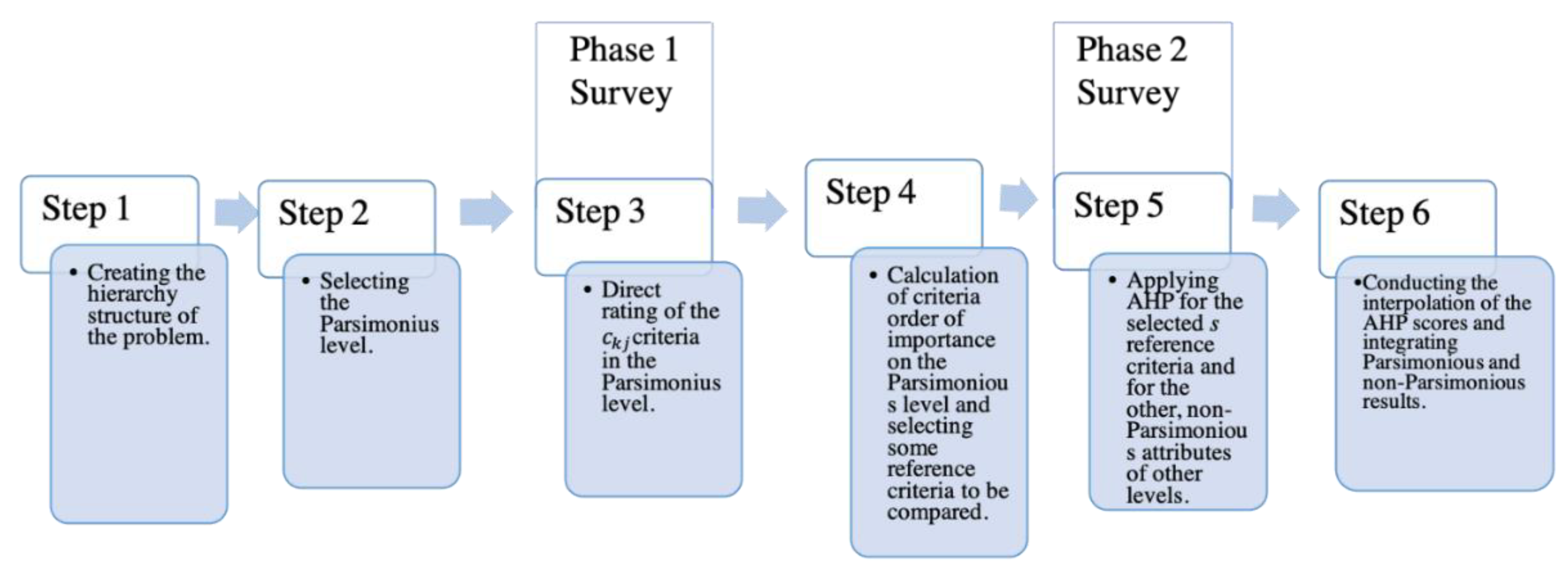[39] to create and present PAHP. Thus, the process of a PAHP survey can be constructed in the following steps.

• Direct rating of the n attributes on a scale from 0 to 100 from the aspect of their importance in the decision. For multilevel decision hierarchy, these scores have to be normalized level wisely to gain the score of each attribute within the respective level.
• Selecting some reference criteria for checking the inner logic in the evaluations and for possible modifications.
• For the reference criteria, AHP has to be conducted, so pairwise comparisons have to be made.
• For these pairwise comparisons, consistency has to be checked by CR, and also the monotonicity of direct ratings and AHP ratings has to be compared. If the consistency or the monotonicity is not fulfilled, the evaluators can modify their ratings to reach robust results.
• In case the robust direct rating and AHP scores are reached, finally the interpolation of the AHP scores is to be conducted for the direct evaluations. By this interpolation, the rank reversal problem is completely avoided, and the direct results are modified by keeping the original ranking.

3.3. The Proposed Multi-Level Parsimonious AHP Technique

Let us have n criteria structured in a decision problem into m levels. Select the k-th level of the structure to be the Parsimonious level of the model. We suggest selecting the level which has more than nine criteria. Let us denote j the criteria on the selected level of the decision so $c_{kj}$ denotes a criterion on the Parsimonious level in which if we have h criteria, j = 1, …, h.

The reason for selecting that level(s) which has h ≥ 9 is that it can be considered as a sufficient number of criteria worth for unburdening the evaluators from numerous pairwise comparisons. Moreover, we propose (following Saaty’s 7 ± 2 rule (Aczel and Saaty, 1983 [41]) for a PCM) to select level(s) for which larger or equal to 5 × 5 pairwise comparison matrices should be evaluated. As recommended protocol, the pair wise comparisons for a 5 × 5 matrix might be demanding for layman evaluators.

In the second step, direct evaluations have to be made for the chosen level(s) for the $c_{kj}$ criteria with respect to the goal of the decision problem on a scale from 0 to 1 or equivalent, e.g., 0–100. By their normalization, we gain the γ$\left(c_{kj}\right)$ values. Please, see the next, case study section. Having gained the normalized values of the criteria, we set up an increasing order and denote the criteria in this order by $c_{kp}$, where p denotes the new position of the criterion, p = 1, …, h.

Then, $t_p$ reference elements have to be selected on the chosen level(s) k based on their new order; we recommend $t_p$ = 3 and to select $c_{k1}$, $c_{kh/2}$ and $c_{kh}$. Thus, s = ($c_{k1}$,$c_{kh/2}, c_{kh})$, and more generally, s = ($s_1$,$s_2,\dots , s_{tp})$. Note that in case of a significantly larger h, the number of selected elements can be larger up to 4 or even 5.

Afterwards, the original AHP pairwise comparisons are conducted for the chosen $t_p$ number of criteria, obtaining the normalized AHP scores for the s criteria: $u\left({\mathrm{c}}_{ks}\right)$, for all s = ($c_{k1}$,$c_{kh/2}, c_{kh})$. Please see the next, case study session. The normalized results of the AHP calculation are denoted by u.

Following the PAHP procedure by Abastante et al. [39], consistency and monotonicity are being checked, and the required modifications are made.

Finally, the following formula is applied for all criteria ($c_{kp}$) existing on the Parsimonious level(s) using the following:

$$u\left(c_{kp} \right)=u\left({\mathrm{c}}_{ke}\right)+\frac{u \left({\mathrm{c}}_{ke+1}\right)-u \left({\mathrm{c}}_{ke}\right)}{{\mathsf{\gamma }}_{ke+1}-{\mathsf{\gamma }}_{ke}} \left({\mathrm{r}}_{kp}-{\mathsf{\gamma }}_{ke}\right).$$

(6)

with respect to e = 1, …, $t_p,$ and $c_{kp}$ has the importance between the two reference criteria $c_{ke}$ and $c_{ke+1}$; thus, $r_{ke}<r_{kp}<r_{ke+1}$ (e = p − 1). In addition, ${\mathsf{\gamma }}_{ke+1}$ and ${\mathsf{\gamma }}_{ke}$ are the normalized direct evaluations of the reference criteria and ${\mathrm{r}}_{kp}$ the normalized direct evaluation of the criterion of interest. Note that the symbol u denotes the normalized AHP value in all cases. Please, see the next, case study section.

Having finished with the Parsimonious level(s), the decision structure should be reconstructed in order to gain the final weight and alternative scores and ranking. Consequently, all $u\left(c_{kp}\right)$-s have to be multiplied by the weight score of their respective element from the previous level k-1. Moreover, due to the characteristics of AHP, for the lower levels, the new $u\left(c_{kp}\right)$ weight scores have to be applied for multiplying the scores of the respective lower elements.

For better understanding, we provide the proposed general flow chart of the multi-level PAHP surveys (Figure 1).

3.4. Spearman’s Rank Correlation Coefficient

For determining the grade of similarity between the new PAHP model results and a previous AHP survey conducted in the same city on the same public bus transport system, we added a nonparametric rank statistic technique [42] and calculated the Spearman’s rank correlation coefficient (R).

Generally, the following is formula used as a mathematical notation for Spearman rank calculation:

$$R=1-\left(\frac{6\sum d^2}{m^3-m}\right)$$

(7)

where d is the difference between ranks, and m is the number of the ranked elements.

The result of the Formula (7) is always between one and minus one. Plus one refers to a perfect positive correlation, and minus one refers to a perfect negative correlation, while zero represents the lack of correlation of the compared rankings.

4. Results of the Parsimonious AHP Survey

In 2019, between the 6th and the 27th of December, we applied the introduced PAHP methodology in a survey on passenger satisfaction with public bus transportation, in the Turkish big city, Mersin. The hierarchical decision structure of satisfaction attributes was exactly the same as in a previous conventional AHP survey in 2019, between the 5th of October and the 4th of November. The new Parsimonious AHP procedure, however, contained some simple pairwise comparisons and also some direct evaluations for the selected Parsimonious level (second in the hierarchy; see Figure 1), and the other levels were not altered from the previous case.

We conducted short personal interviews in two phases at bus stops along the main public bus lines of Mersin. The first phase targeted specifically the Parsimonious level of the hierarchy and contained direct evaluations of the second level elements in the structure. The second phase aimed to conduct the necessary pairwise comparisons between the supply quality elements on the other levels and the pairwise comparisons of the selected attributes on the Parsimonious level. The first phase was conducted in one week, and the second in two weeks. During the three weeks, 500 + 500 responses were collected from two patterns with the following characteristics (

Table 3. Respondents’ characteristics of the first round.

Passengers = 500			%
Gender	Male	258	51.6
	Female	242	48.4
Marital status	Married	186	37.2
	Single	314	62.8
Age	18–30 years	313	62.6
	31–55 years	139	27.8
	>55 years	48	9.6
Education level	Primary school	12	2.4
	Secondary school	15	3
	High school	184	36.8
	Bachelor’s degree	257	51.4
	MSc/PhD degree	32	6.4
Working status	Student	231	46.2
	Employee in private sector	98	19.6
	Employee in public sector	107	21.4
	Retired	64	12.8
Frequency of use	1–5 trips/week	59	11.8
	5–20 trips/week	291	58.2
	21–30 trips/week	139	27.8
	>30 trips/week	11	2.2

for first round survey and

Table 4. Respondents’ characteristics of the second-round pattern.

Passengers = 500			%
Gender	Male	252	50.4
	Female	248	49.6
Marital Status	Married	179	35.8
	Single	321	64.2
Age	18–30 years	321	64.2
	31–55 years	135	27
	>55 years	44	8.8
Education level	Primary school	9	1.8
	Secondary school	11	2.2
	High school	178	35.6
	Bachelor’s degree	264	52.8
	MSc/PhD degree	38	7.6
Working status	Student	243	48.6
	Employee in private sector	93	18.6
	Employee in public sector	104	20.8
	Retired	60	12
Frequency of use	1–5 trips/week	56	11.2
	5–20 trips/week	297	59.4
	21–30 trips/week	133	26.6
	>30 trips/week	14	2.8

for the second round).

Both patterns are somewhat similar to the demographic situation of Mersin and definitely similar to the typical public transport users [43] of the city (dominantly young students and employees).

The average time of evaluations was around 5 min in the first phase and was 15 min in the second but did not exceed 20 min in any case. The response rate was very high in both rounds with an estimated proportion of 90%, probably due to the instructor applied and the personal contact. Moreover, the consistency of the responses was high, since the instructor could answer any questions referred to the understanding of the meaning and mode of evaluation. The construction of the questionnaire followed the PAHP approach for the following model of passenger satisfaction.

Step 1:Figure 2 demonstrates that we have applied 24 attributes structured into three levels to characterize the supply quality of public bus transportation. The respondents compared the importance of these attributes in terms of the necessity of their development. For a conventional AHP survey, the questionnaire would have contained the level wise and branch wise pair wise comparisons of all the elements of the decision structure by the values of the well-known Saaty-scale (from 1 to 9 to express superiority and from ½ to 1/9 to express inferiority).

However, in our approach, the second level, which contained the most attributes (11) and the branch with most attributes (five), has been selected as Parsimonious level (Step 2). For these elements, the direct evaluations, the pair wise comparisons for few (three) reference elements and the interpolation technique presented in the Methodology section (see Formula (6)) have been applied in a later step.

For the Parsimonious level, we have applied the PAHP approach here, in the first round of surveying. In this third step (Step 3), the 11 $c_{kj}$ criteria have been directly evaluated (level wisely “level 2”) by passenger evaluators (500) based on (0–10) scale. The characteristics of the respondent pattern for this first survey round is presented by Table 3.

During Step 4, we normalized the gained scores to 1 for all 11 attributes of this level.

Table 5. The gained normalized direct evaluation by passenger raters (γ$(c_{kj})$).

Criteria	The Normalized Direct Evaluation
Mental comfort	0.052
Approachability	0.058
Information during travel	0.057
Time availability	0.078
Speed	0.056
Directness	0.149
Safety of Travel	0.111
Perspicuity	0.103
Physical comfort	0.116
Reliability	0.124
Information before travel	0.096

shows the gained normalized increasing order:

Still in this step, we had to select some reference criteria to be compared in the later stage of multi-level Parsimonious AHP methodology. As selection criteria, the PAHP literature [39,44] recommends keeping the s number of selected attributes low enough for easier pair wise comparisons and, simultaneously, high enough to represent the set of the elements of the Parsimonious level. In this case study, three reference attributes (the most and the least important and an intermediate based on the first direct evaluations) seemed sufficient to select. The attributes: “Information before travel” (${\mathsf{\gamma }}_1=0.096$), “Directness” (${\mathsf{\gamma }}_2=0.149$) and “Mental comfort” (${\mathsf{\gamma }}_3=0.052$) have been chosen.

In Step 5, the selected reference criteria have been compared pair wisely during the second-round survey (see its characteristics in Table 4), following the original AHP approach; the scores are presented in

Table 6. The PCM of the reference criteria gaining the normalized scores of ($u(c_{ks})$).

CR = 0.00258	Information before Travel	Directness	Mental Comfort	Scores	Rank
Information before travel	1	0.278	1.675	0.221	2
Directness	3.597	1	2.911	0.610	1
Mental comfort	0.597	0.344	1	0.169	3

.

The consistency ratio has been calculated and monotonicity has been checked. Based on the results another round for improving consistency has not been necessary since the CR got a value smaller than 0.1 (CR = 0.00258), which is considered consistent enough in AHP literature, and the monotonicity condition has also been completed. (Note that the rank of the three criteria remained the same after the pairwise comparisons).

Still in this step, within the frames of the second-round survey, the evaluators have been asked to compare pair wisely the three attributes of the first and the third level. Based on the conventional AHP approach, in the first level, three questions have been asked: please compare the relative importance of Transport Quality to Service Quality in terms of their need for improvement, and do the same for Service Quality and Tractability and for Transport Quality and Tractability. Obviously, due to reciprocity, it has been unnecessary to ask in the other direction. The calculation of the results has also been exactly the same as in the conventional AHP process for the attributes of the third, non-Parsimonious level. In Step 6, the priorities for all the criteria have been obtained (the comprehensive evaluation was done by employing Formula (6)) within the interval we have repositioned all other criteria scores.

$$u\left(\mathrm{Approachability}\right)=0.169+\frac{0.221-0.169}{0.096-0.052} \left(0.058-0.052\right)=0.169+\frac{0.052}{0.044} \left(0.006\right)=0.176$$

$$u\left(\mathrm{Reliability}\right)=0.221+\frac{0.610-0.221}{0.149-0.096} \left(0.102-0.096\right)=0.221+\frac{0.389}{0.053} \left(0.006\right)=0.427$$

Consequently, the ranking order has been kept for all criteria in the Parsimonious level.

Before determining the final scores in the decision, the original decision structure (see Figure 2) has to be rebuilt. Based on this, the final Parsimonious scores have to be normalized by their position in the original hierarchy. For instance, the Parsimonious score of Approachability, Directness, Time availability, Speed and Reliability have to be normalized to 1 (

Table 7. The direct evaluation by passengers and the final Parsimonious scores ($u(c_{kp})$) of the criteria in level 2.

Criteria	Direct Evaluation	Rank	$\mathbf{Parsimonious}\mathbf{Scores}(\mathit{u}({\mathit{c}}_{\mathit{k}\mathit{p}}))$
Approachability	0.058	8	0.176
Directness	0.149	1	0.610
Time availability	0.078	7	0.200
Speed	0.056	10	0.174
Reliability	0.124	2	0.427
Physical comfort	0.116	3	0.368
Mental comfort	0.052	11	0.169
Safety of travel	0.111	4	0.331
Perspicuity	0.103	5	0.272
Information before travel	0.096	6	0.221
Information during travel	0.057	9	0.175

). Moreover the other, non-Parsimonious levels and criteria scores have to be attached to the decision.

The other normalized scores for the elements in the Parsimonious level which obtained by the PAHP approach are calculated based on Formula (6). As following (

Table 8. Level 1 and Level 3 scores obtained from the conventional AHP approach; Level 2 scores obtained from the PAHP approach.

Level 1		Level 2 (Parsimonious Level)		Level 3
Supply Quality		Service Quality		Approachability
Service Quality	0.406	Approachability	0.176	Directness to stop	0.456
Transport Quality	0.238	Directness	0.610	Safety of stops	0.213
Tractability	0.356	Time availability	0.200	Comfort in stops	0.331
		Speed	0.174	Directness
		Reliability	0.427	Need of transfer	0.622
		Transport Quality		Fit connection	0.378
		Physical comfort	0.368	Time availability
		Mental comfort	0.169	Frequency of lines	0.723
		Safety of travel	0.331	Limited time of us	0.277
		Tractability		Speed
		Perspicuity	0.272	Journey time	0.257
		Info before travel	0.221	Awaiting time	0.491
		Info during travel	0.175	Time to reach stops	0.252

):

$$u\left(\mathrm{Time}\mathrm{availability}\right)=0.169+\frac{0.221-0.169}{0.096-0.052} \left(0.078-0.052\right)=0.2$$

$$u\left(\mathrm{Speed}\right)=0.169+\frac{0.221-0.169}{0.096-0.052} \left(0.056-0.052\right)=0.174$$

$$u\left(\mathrm{Physical}\mathrm{comfort}\right)=0.221+\frac{0.610-0.221}{0.149-0.096} \left(0.116-0.096\right)=0.368$$

$$u\left(\mathrm{Safety}\mathrm{of}\mathrm{travel}\right)=0.221+\frac{0.610-0.221}{0.149-0.096} \left(0.111-0.096\right)=0.331$$

$$u\left(\mathrm{Perspicuity}\right)=0.221+\frac{0.610-0.221}{0.149-0.096} \left(0.103-0.096\right)=0.272$$

$$u\left(\mathrm{Info}\mathrm{during}\mathrm{travel}\right)=0.169+\frac{0.221-0.169}{0.096-0.052} \left(0.057-0.052\right)=0.169+1.182 \left(0.005\right)=0.175$$

Based on this, the final decision scores and ranking can be obtained and the multi-level PAHP problem can be solved. We note again that the first level in the decision structure is obviously equals to the AHP scoring.

According to the PAHP approach outcomes, the final scores and the criteria ranking are presented in

Table 9. Level 1 and Level 3 scores obtained from the conventional AHP approach; Level 2 scores obtained from the PAHP approach after normalization.

Level 1		Level 2 (Parsimonious Level)		Level 3
Supply Quality		Service Quality		Approachability
Service Quality	0.406	Approachability	0.111	Directness to stop	0.456
Transport Quality	0.238	Directness	0.385	Safety of stops	0.213
Tractability	0.356	Time availability	0.126	Comfort in stops	0.331
		Speed	0.110	Directness
		Reliability	0.269	Need of transfer	0.622
		Transport Quality		Fit connection	0.378
		Physical comfort	0.424	Time availability
		Mental comfort	0.195	Frequency of lines	0.723
		Safety of travel	0.381	Limited time of us	0.277
		Tractability		Speed
		Perspicuity	0.408	Journey time	0.257
		Info before travel	0.331	Awaiting time	0.491
		Info during travel	0.262	Time to reach stops	0.252

and

Table 10. Final normalized scores by passengers for level 2 (after their normalization by branches).

Criteria	Level 2
	Scores	Rank
Approachability	0.045	10
Directness	0.156	1
Time availability	0.051	8
Speed	0.044	11
Reliability	0.109	4
Physical comfort	0.101	5
Mental comfort	0.046	9
Safety of travel	0.091	7
Perspicuity	0.145	2
Information before travel	0.118	3
Information during travel	0.093	6

. Table 10 exhibits the final scores for the second level of the decision structure which are calculated by multiplying the scores by their branch scores. The sensitivity analysis has been applied by changing the weight of each main criterion to detect the stability of the ranking, and it has been robust without change.

Table 11. Final normalized scores by passengers for level 3 (after their normalization by branches).

Criteria	Level 3
	Scores	Rank
Directness to stops	0.021	5
Safety of stops	0.010	10
Comfort in stops	0.015	6
Need of transfer	0.097	1
Fit connection	0.059	2
Frequency of lines	0.037	3
Limited time of use	0.014	7
Journey time	0.0114	8
Awaiting time	0.022	4
Time to reach stops	0.0112	9

exhibits the final scores for the last level of the decision structure which are calculated by multiplying the element’s scores by their branch scores:

4.1. A New Hierarchical Analysis on the Multi-Level PAHP Results

In case of multi-level Parsimonious AHP modelling, the possibility of testing the Parsimonious level results in the frame of the hierarchy provides the opportunity of a hierarchical analysis. As the parsimonious scores are obtained by a different computational process and not by full pairwise comparisons as in AHP, comparing the sum of normalized criteria scores with the respective upper-level criterion score provides valuable extra information on the final priority.

The analysis resulted in a significant extra information on the scores (see

Table 12. Hierarchical analysis of PAHP scores.

Level 1		Level 2 (Parsimonious Level)
Supply Quality		Service Quality
Service Quality	0.406	Approachability	0.176
Transport Quality	0.238	Directness	0.610
Tractability	0.356	Time availability	0.200
		Speed	0.174
		Reliability	0.427
		Sum Service Quality: 1.587
		Transport Quality
		Physical comfort	0.368
		Mental comfort	0.169
		Safety of travel	0.331
		Sum Transport Quality: 0.868
		Tractability
		Perspicuity	0.272
		Info before travel	0.221
		Info during travel	0.175
After normalization		Sum Tractability:	0.668
Service Quality 0.508		Total parsimonious	3.123
Transport Quality 0.278
Tractability 0.214

Hierarchical score of Service Quality = Sum of Service Quality/Total parsimonious = 1.587/3.123 = 0.508. Hierarchical score of Transport Quality = Sum of Transport Quality/Total parsimonious= 0.868/3.123 = 0.278. Hierarchical score of Tractability = Sum of Tractability/Total parsimonious = 0.668/3.123 = 0.214.

). During the parsimonious process, the evaluators allocated higher scores (0.508) to Service Quality (through evaluating the components of this criterion) than in the AHP phase for the first level (0.406). Hence, Service Quality might have higher significance in the final decision compared to the original AHP weight. This also refers to Transport Quality because indirectly, its components constitute larger weights than the original first level AHP weight of 0.238. Simultaneously, Tractability might have lower significance compared to the original score of 0.356.

We emphasize that this analysis does not change the calculated ranking and rather sophisticates the computed scores and might serve as sensitivity testing. In creating the final decision, the hierarchical comparison should also be considered by the decision makers.

4.2. Rank Concordance of PAHP and AHP Final Results

To compare the current results of the new PAHP model in 2019 and the new results of the conventional AHP approach in 2019, we calculated the Spearman rank correlation on their rankings. Both surveys have been conducted in the same city, Mersin, with the same survey method, personal interviews applying the same decision elements (Figure 1) on the same public bus transport system. In the interval between the surveys, no significant development of the public transport system could be detected.

Table 13. Comparison of the reference conventional AHP survey and the new PAHP survey.

	2019 AHP Survey	2019 PAHP Survey
Location	Mersin. Turkey	Mersin. Turkey
Evaluators	Passengers	Passengers
Question technique	personal interviews by an instructor	personal interviews by an instructor
Number of evaluators	500	500 + 500
Number of questions	6 demographic questions +27 PCMs	6 demographic questions + direct evaluation +14 PCMs
Type of questions	Pairwise comparisons	Direct evaluations and few pairwise comparisons
Response rate	under 50%	over 90%
Total duration	29 days	21 days
Average time of filling	25–30 min	5 + 15 min
Consistency	All PCMs were consistent	All PCMs were consistent

presents the comparison of technical details of the two studies.

The final weight scores for all criteria based on the conventional AHP approach are presented in the following tables (

Table 14. The final weight scores by passengers for level 1 based on conventional AHP.

Criteria	Scores	Rank
Service Quality	0.3980	1
Transport Quality	0.2750	3
Tractability	0.3270	2

,

Table 15. The final weight scores by passengers for level 2 based on conventional AHP.

Criteria	Scores	Rank
Approachability	0.0657	9
Directness	0.1357	2
Time availability	0.0744	8
Speed	0.0414	11
Reliability	0.0808	6
Physical comfort	0.1051	5
Mental comfort	0.0564	10
Safety of travel	0.1136	3
Perspicuity	0.1393	1
Information before travel	0.1082	4
Information during travel	0.0795	6

and

Table 16. The final weight scores by passengers for level 2 based on conventional AHP.

Criteria	Scores	Rank
Directness to stops	0.0273	4
Safety of stops	0.0156	8
Comfort in stops	0.0229	5
Need of transfer	0.0955	1
Fit connection	0.0402	3
Frequency of lines	0.0576	2
Limited time of use	0.0168	6
Journey time	0.0145	9
Awaiting time	0.0166	7
Reaching time	0.0103	10

):

In the following, the rank comparison between the results is presented. For the first level, the R value is plus one, which represents a perfect positive correlation, which is a strong averment to show the efficiency of the PAHP approach. The positive correlation was not only detected on the first level but also on the second and third levels; moreover, on the second level a strong positive correlation (R = 0.829) could be detected, and on the third level also a strong positive correlation (R = 0.825) could be obtained.

Table 17. Spearman’s Rank correlation coefficient for Level 1.

Criteria	Rank of 2019 AHP Survey	Rank of 2019 PAHP Survey	${\mathit{d}}_{\mathit{i}}$	${\left({\mathit{d}}_{\mathit{i}}\right)}^2$
Service quality	2	2	0	0
Transport Quality	1	1	0	0
Tractability	3	3	0	0
m = 3		R = 1

,

Table 18. Spearman’s Rank correlation coefficient for Level 2.

Criteria	Rank of 2019 AHP Survey	Rank of 2019 PAHP Survey	${\mathit{d}}_{\mathit{i}}$	${\left({\mathit{d}}_{\mathit{i}}\right)}^2$
Approachability	9	10	19	1
Directness	2	1	3	225
Time availability	8	8	16	4
Speed	11	11	22	16
Reliability	6	4	10	64
Physical comfort	5	5	10	64
Mental comfort	10	9	19	1
Safety of travel	3	7	10	64
Perspicuity	1	2	3	225
Information before travel	4	3	7	121
Information during travel	6	6	12	36
m = 11		R = 0.829

and

Table 19. Spearman’s Rank correlation coefficient for Level 3.

Criteria	Rank of 2019 AHP Survey	Rank of 2019 PAHP Survey	${\mathit{d}}_{\mathit{i}}$	${\left({\mathit{d}}_{\mathit{i}}\right)}^2$
Directness to stops	4	5	9	56.25
Safety of stops	8	10	18	2.25
Comfort in stops	5	6	11	30.25
Need of transfer	1	1	2	210.25
Fit connection	3	2	5	132.25
Frequency of lines	2	3	5	132.25
Limited time of use	6	7	13	12.25
Journey time	9	8	17	0.25
Awaiting time	7	4	11	30.25
Time to reach stops	10	9	19	6.25
m = 10		R = 0.825

show the computed correlation outcomes between AHP and PAHP.

It could be stated that the comparison of the AHP and PAHP results has been very successful, since for all levels, the two rankings correlate very strongly. Moreover, we highlight that due to the nature of AHP and PAHP, only a slight difference in the weight scores on the upper levels causes rank reversal on the lower levels. Considering this feature, the performance of the new PAHP technique is even more convincing. The ranking on the first level is exactly the same. Although on the second level the top three positions are slightly modified by the new model, the significant role of Directness, Safety of travel, Perspicuity and Physical comfort are highlighted in both cases. Further, taking into account the overall priorities, the 0.829 concordance is very high in the case of two surveys with different patterns conducted in different time. The two priorities for the third level attributes show also very high concordance with the value of 0.825. The top three positions are almost the same except for a change in the second and third ranks.

5. Conclusions

This paper aimed to demonstrate as pioneer a new multi-level PAHP survey process, maintaining the benefits of AHP but mitigating some of its disadvantages by the creation of a new, Parsimonious AHP based model and procedure. As for all passenger satisfaction surveys, the objective was to gain as much consistent information as possible by keeping the efforts of the respondents and consumed time and cost low, while keeping response rate and accuracy high.

Based on the results, it can be concluded that the new PAHP based model produced very similar results to those of a previous, conventional AHP survey with significantly strong overall rank correlation accompanied with a convincing performance in selecting the most significant decision elements for all three levels.

This performance could be reached by a shorter total survey duration (21 days versus 29 days), less individual evaluation time (5 + 15 min versus 25–30 min) but a much higher response rate (over 90% versus 50%) and consequently by a much efficient survey process.

As limitation, evidently, the uniqueness of the research has to be noted. Many other PAHP surveys are still necessary to further sophisticate the process and to state that this new methodology can be a competitor of the widely applied AHP technique. However, based on this sole application, it can be concluded that the results from the cost–benefit point of view are more than promising.

The adopted model can be utilized in all science fields in order to deal with complex problems after constructing a suitable hierarchy for these problems.

For further research, we plan to repeat this survey but without the human help of an instructor, using an automated technology instead, for instance, smartphone-based evaluations by a QR code positioned on public bus vehicles, and thus extend the pattern of evaluators significantly.