Article

Behaviour Investigation of SMA-Equipped Bar Hysteretic Dampers Using Machine Learning Techniques

by
Visar Farhangi
1,
Hashem Jahangir
2,*,
Danial Rezazadeh Eidgahee
3,*,
Arash Karimipour
4,
Seyed Alireza Nedaei Javan
5,
Hamed Hasani
2,
Nazanin Fasihihour
6 and
Moses Karakouzian
1
1
Department of Civil and Environmental Engineering and Construction, University of Nevada, Las Vegas, NV 89154, USA
2
Department of Civil Engineering, University of Birjand, Birjand 97174-34765, Iran
3
Faculty of Civil Engineering, Semnan University, Semnan 35131-19111, Iran
4
Member of Centre for Transportation Infrastructure Systems (CTIS), Department of Civil Engineering, University of Texas at El Paso, El Paso, TX 79968, USA
5
Civil Engineering Department, Hormozan University of Birjand, Birjand 97148-83385, Iran
6
Department of Telecommunication and Electronics, University of Politecnico di Torino, 10129 Torino, Italy
*
Authors to whom correspondence should be addressed.
Appl. Sci. 2021, 11(21), 10057; https://doi.org/10.3390/app112110057
Submission received: 16 August 2021 / Revised: 21 October 2021 / Accepted: 25 October 2021 / Published: 27 October 2021
(This article belongs to the Special Issue Applications of Deep Learning in Engineering Structures)

Abstract

:
Most isolators have numerous displacements due to their low stiffness and damping properties. Accordingly, the supplementary damping systems have vital roles in damping enhancement and lower the isolation system displacement. Nevertheless, in many cases, even by utilising additional dampers in isolation systems, the occurrence of residual displacement is inevitable. To address this issue, in this study, a new smart type of bar hysteretic dampers equipped with shape memory alloy (SMA) bars with recentring features, as the supplementary damper, is introduced and investigated. In this regard, 630 numerical models of SMA-equipped bar hysteretic dampers (SMA-BHDs) were constructed based on experimental samples with different lengths, numbers, and cross sections of SMA bars. Furthermore, by utilising hysteresis curves and the corresponding ideal bilinear curves, the role of geometrical and mechanical parameters in the cyclic behaviour of SMA-BHDs was examined. Due to the deficiency of existing analytical models, proposed previously for steel bar hysteretic dampers (SBHDs), to estimate the first yield point displacement and post-yield stiffness ratio in SMA-BHDs accurately, new models were developed by the artificial neural network (ANN) and group method of data handling (GMDH) approaches. The results showed that, although the ANN models outperform GMDH ones, both ANN- and GMDH-based models can accurately estimate the linear and nonlinear behaviour of SMA-BHDs in pre- and post-yield parts with low errors and high accuracy and consistency.

1. Introduction

There are several techniques that can be used for improving seismic behaviour in structures [1,2,3,4]. Adding certain elements to the structure, such as shear walls or steel braces, would enhance the seismic strength of the structure. Due to this fact, the lateral stiffness of the structure is increased, and the increased lateral stiffness will develop the force applied to major structural components [5,6,7]. Increasing the seismic behaviour of structures can be enhanced by insulating the foundations from the supports. Despite strengthening strategy of structural elements affected by lateral loads, isolated structural elements without any strengthening could be an alternative. When the seismic demand in isolated systems is reduced, the structural performance can be enhanced without affecting main elements by increasing their internal forces. For the isolators to withstand the vertical forces of the structure, they should be sufficiently stiff in the vertical direction [8,9,10]. Although to reduce the overall lateral stiffness of the structure and increase its time period, the stiffness isolators should be significantly lower horizontally than vertically. Isolators, in general, are low dampened, and adding additional dampers in some circumstances can increase dampening and decrease the displacement of the isolation systems [11]. Despite causing an increase in the force applied to the isolation system, utilising added dampers may generally minimise the displacement of the whole structure. Therefore, dampers and their impact on the performance of isolated structures should be thoroughly examined [12]. Recently, some new machine learning and artificial intelligence techniques were utilised to solve complicated civil engineering problems related to bridges [13,14,15].
There are different kinds of dampers, among which are steel hysteretic dampers, which attract the interest of many researchers due to their durable hysterical behaviour, high potential in energy dissipation, long-term robustness, low production cost, and simple replacement and installation [16,17]. In these dampers, plastic deformation occurs through bending, shear, torsion, or the aforementioned mechanisms that deal with energy dissipation. Researchers such as Guerrero [18], Muto [19], Kelly et al. [20], and Skinner et al. [21] were the first to introduce the idea of using steel as a damper. Known as the added damping and stiffness (ADAS) tool, it has been introduced in several types; Bergman and Goel [22] developed a well-known type of damper with X-shaped steel plates and connected parallel to base plates of structures. The triangular-shape-added damping and stiffness (TADAS) was then introduced by Tsai et al. [23]. Similar to the ADAS dampers, in TADAS dampers, both ends of steel triangles are attached to the base plates. Many other researchers investigated the behaviour of ADAS X-shaped and triangular dampers [24,25]. Shin et al. [26] and Shin and Sung [27] proposed the rhombic ADAS dampers using low-strength steel with pinned joints at each end. Their observation was that the pinned joints at both ends of the damper prevent the plate from being subjected to unwanted axial forces. In addition, the mechanical characteristics of low-strength steel improve energy absorption and damper ductility. Han et al. [28] conducted additional experiments on rhombic ADAS dampers. The slit steel damper (SSD), composed of a wide flanged steel section with seamless rounded ends, was proposed by Chan and Albermani [29]. Other research works have also been conducted to evaluate steel damper behaviour [30,31,32,33,34,35]. A shear panel damper (SPD), which contains a steel plate linked to two upper and lower panels, has also been proposed and investigated by some researchers [36,37,38,39,40,41]. Garivani et al. [42] developed a comb-teeth damper (CTD), which comprises steel plates that resemble comb teeth. During in-plane bending, the yielding process of teeth in these dampers could cause energy dissipation. The E- and C-shaped tools, which dissipate energy due to the plastic deformation of steel materials, were employed as a damper in several other investigations [43]. Kato et al. [44] and Kato and Kim [45] employed steel J-shaped sheets as dampers, which allow the energy to be dissipated by yielding of steel plate under the roll bending. In several research works, U-shaped components were also employed as steel hysteretic dampers [46,47,48,49,50,51,52,53].
Recently, steel bars are also used as a novel type of hysteretic dampers, in which the two ends of steel bars are connected to two steel plates in order to dispel energy through the bending deformations mechanism. In addition to Ghaedi et al. [54,55], Aghlara and Tahir [56] evaluated the steel bar dampers with repair capability of bar substitution. The obtained results indicate that steel bar dampers have a high ability to dissipate energy and withstand significant deformations. In an experimental study, Golzan et al. [57] considered the steel bar hysteretic dampers (SBHD) as added dampers to elastomeric isolators and proposed a simple method to design them. Jahangir et al. [58] conducted a comprehensive numerical study on the role of geometrical parameters in SBHD dampers. SBHD with steel bars of different lengths, numbers, and cross sections were analysed in their study, and the seismic behaviour was investigated by utilising hysteresis curves. Moreover, using the multiple nonlinear regression (MNLR) methods, some models were proposed to estimate the behaviour of SBHDs in pre- and post-yielding point sections.
Steel bar hysteretic dampers (SBHDs), as added dampers to isolation systems, could withstand strong earthquakes, but the residual displacements result in higher repair costs, lower safety levels, and a significant decline in the ability of SBHD-equipped structures to withstand aftershocks. To overcome this problem, externally bonded composites can strengthen structural components [59,60,61,62,63,64]. For the near-fault areas with greater seismic risks, a substation of steel bars with shape memory alloys (SMAs) with recentring properties may be a better option. Scientists found that SMA materials could withstand significant nonlinearities and return to their original shape after unloading. As a result of their excellent corrosion resistance, fatigue resistance, and damping capacity [65], these materials reduce maintenance costs. The use of SMAs for structural purposes has been assessed through some studies throughout the past several decades, including damping devices [66], bridge supports [67,68,69], vibrational damage detection systems [70], reinforcement systems [65,71,72,73,74], and systems of seismic isolation [75]. On the opposite of SMA advantages in improving structural behaviour, earlier studies have demonstrated that SMAs usage poses certain drawbacks as a steel bar in SBHDs. In particular, large-diameter SMAs rebar is difficult to manufacture due to their great hardness [76]. Moreover, due to the fragility of the connecting point in SMA bars, they cannot be welded to steel sections [77]. Therefore, one of the most challenging aspects of using SMAs is the high preparation costs. Despite a decline in price over the past decade, the price for these alloys remains expensive when compared with other contemporary materials. As a result, SMAs are usually used in an optimum manner only in places where more deformation is experienced.
Despite several studies conducted on various hysteretic dampers with various geometric shapes, there are still some questions regarding their behaviour, and in particular their behaviour with steel bars. Moreover, the residual displacements in steel bar hysteretic dampers (SBHDs) increase the maintenance and repair costs after earthquakes occurrence. Utilising shape memory alloys (SMAs) as a smart material with recentring properties and less residual displacement with respect to steel bars could be a proper alternative. As the prices of SMAs are more than steel materials, their usage should be conducted in an optimum manner. To address these gaps, this study proposed a novel developed bar hysteretic damper as an added damper to an isolation system, in which the steel bars are substituted optimally by SMA bars with different mechanical properties and geometrical configurations. A comprehensive study was conducted to evaluate the role of different geometrical such as the length, number, and cross section of the SMA bars on the cyclic behaviour of SMA-equipped bar hysteretic dampers (SMA-BHDs). After evaluating existing analytical models for identifying the mechanical characteristics of SMA-BHDs, new alternative models with higher accuracy and lower error values were proposed by utilising different machine learning methods.

2. Shape Memory Alloys

Shape memory alloys (SMAs) are considered smart and innovative materials discovered as early as 1932 and, in 1960, were manufactured from nickel and titanium [78] to exhibit better behaviour than any other element used in memory alloys. These polymorphic materials are composed of crystalline or chemical phases. SMAs are capable of enduring large stresses without causing residual strains, and it is efficient in dissipating energy [79]. In shape memory alloys, the prevailing crystalline phase is dependent on the temperature and stress. Austenite and martensite are the two crystalline phases of SMAs. Austenite and martensite phases are stable at high and low temperatures and low and high stresses, respectively [80]. Therefore, these two phases could be transformed into each other through a heating process or by applying mechanical forces. SMAs exhibit different macroscopic behaviour during the transition from one phase to another. There are certain characteristics that distinguish SMAs from other alloys and metals, specifically, shape memory and superelasticity features. SMAs’ mechanical behaviour under different levels of stress and strain and various temperatures is shown in Figure 1. A shape memory feature is present in SMAs at temperatures below the austenite-transformation-to-martensitic phase during cooling, Mf, and the superelasticity feature is created when the temperature is above the finish temperature of the martensite-transformation-to-austenite phase during heating, Af [79]. At temperatures below Mf and in the martensitic phase, SMAs deform under stress. By load removal, the alloy could not return to its original shape and would experience residual strains. In this case, named the one-way shape memory feature, the martensitic phase is still dominant in SMAs.
In a one-way shape memory feature, just heating and cooling processes could convert the martensite and austenitic phases into one another without stress being applied. This case in which SMAs could remember their different shapes at high and low temperatures is named the two-way shape memory feature. SMAs with two-way shape memory characteristics are among the few that exist and are utilised in temperature-sensitive actuators and reversible fasteners in medical research fields [78,80]. By applying stresses, the austenitic phase of SMAs would be transformed into the martensitic phase at a higher temperature than Af and lower than Md (a higher temperature than Af, at which the alloy has an elastoplastic feature). As shown in Figure 1, unloading in this situation leads to an unstable martensitic phase, which undergoes an inverse transformation that leads SMAs to return to their original state with no residual strain. This feature is named superelasticity and is utilised in many engineering fields [79].
Researchers used this smart material in many different fields due to austenitic to martensitic transformation, resulting in shape memory and superelasticity properties. The superelasticity property of SMAs is used in this study to improve the seismic behaviour of bar hysteretic dampers utilising the stress–strain model introduced by Auricchio and Sacco [81] and also used in finite element SeismoStruct software [82]. As presented in Figure 2, the most important parameters in this model are σfEA (stresses relating to the beginning transformation of the austenitic into the martensitic phase), σsSA (stresses linked to the end of the austenitic phase into the martensitic phase transformation), σsAS (stresses related to the beginning of unloading step), σfAS (stresses relating to the ending of the unloading step), εl (strain equivalent at the unloading step) and ESMA (elastic modulus in the austenitic phase) [81].

3. Methodology

In this paper, ANN and GMDH-NN were employed to estimate the cyclic behaviour of SMA bar hysteretic dampers. The overall search flowchart in this paper is depicted in Figure 3.

3.1. The Artificial Neural Networks (ANNs)

To address complex engineering issues, artificial neural networks (ANNs) are commonly used in machine learning techniques [83,84]. It is possible to think of a neural network as a set of processes that turn inputs into outputs [85]. The ANNs are constructed by duplicating biological neural networks, which can be trained using input and output data sets [86]. To achieve a certain degree of accuracy, the neural network must be trained in order to update the correlation weights and biases. The overall structure of ANN could be seen in Figure 4, which consists of input layers (X1 to Xn), as well as an output layer (Y) and several hidden layers [87]. It is then determined whether the model is acceptable for output estimation once it has been trained, and its weights have been tested on a separated unseen dataset [88].

3.2. The Group Method of Data Handling (GMDH)

According to Volterra functional series, the relationship between input and output variables may be estimated differently from the ANN method. The discrete equivalent of the Volterra functional series is Kolmogorov-Gabor polynomials [89].
Y = a 0 + i = 1 n a i X i + i = 1 n j = 1 n a i j X i X j + i = 1 n j = 1 n k = 1 n a i j k X i X j X k +
where A vector of weights is defined as a = (a0, a1, ..., an) for input variables X = (X1, X2, ..., Xn). Despite its ability to approximate any stationary random series of observations, the Kolmogorov–Gabor polynomial has two disadvantages. A lengthy and incomplete vector of independent variables is most common, whereas the collection of observations is limited. In addition, as the input vector increases in size, the computation time for calculating all the necessary normal equations rises. Inspired by Kolmogorov-Gabor polynomials [89], Ivakhnenko [90] created the group method of data handling (GMDH) as a heuristic self-organisation method. Ivakhnenko strived to enhance the Kolmogorov polynomial using lower orders for each pair, employing heuristic and Perceptron techniques. This approach, which is based on the Perceptron-type structure, is more accurate and allows data classification into useful and harmful categories. As a result, it requires fewer observations and decreases computation time [91]. An adaptive generalised polynomial-based function model is created by GMDH-NN, which advances in complexity over time until it achieves an ideal degree of complexity, at which it is neither too simple to generalise nor too complicated to overfit, which would result in a network, as seen in Figure 5. Using the GMDH v, the number of layers, the nodes that must be selected, and the properties of those nodes are automatically determined.

4. Experimental Specimens and Numerical Models

4.1. Experimental Specimens

In this study, as shown in Figure 6, the experimental study conducted by Golzan et al. [57] on steel bar hysteretic dampers (SBHDs) as an added damper to bridge isolator systems was considered as a reference to conduct the numerical analysis. A vertical load representing gravity loads allowed forces to be applied by two vertical jacks in their test setup. At the same time, the horizontal displacement was applied to the isolation system. The geometry of the test setup was designed to accommodate added damper parallel to the isolator system. The isolation system contained a rubber isolator designed for highway bridge piers in Quebec, Canada. The added damper included six horizontal steel bars of 38 mm diameter and 1.5 m long [57]. The energy absorption mechanism in this damper occurred when the cross section of bars reached the nonlinear range in bending, and plastic hinged induced in their two ends and mid-length. More comprehensive details regarding the experimental test setup can be found in Jahangir et al. [58] research.
The seismic behaviour of isolation systems equipped using SBHDs was investigated by applying a predefined cyclic load pattern, as shown in Figure 7. In the first step, to study the isolator behaviour, the steel bar hysteretic dampers were not added to rubber isolators [57].

4.2. Numerical Models

In this paper, considering the experimental study conducted by Golzan et al. [57], the numerical models of isolation systems and SBHDs were generated in the SeismoStruct software to determine whether the software could achieve the expected results [82]. In these models, the same cyclic loading pattern presented in Figure 7 was applied, and using the software link element, the rubber isolator was simulated by a bilinear spring. On the other hand, since this study seeks the influence of geometrical parameters on the cyclic behaviour of bar hysteretic dampers, according to Figure 8, the steel bars were precisely modelled by SeismoStruct software.
Figure 8 shows that steel bars are integrated into the isolation system by passing through orifices of a loading plate (Loading Plate) subjected to cyclic loads. According to the experimental test setup, each free ends of the bars are restrained by two plates (Bearing Plates) from lateral movement and rotation (from the experiment supports). Based on the mechanical characteristics of steel materials reported in Golzan et al. [57] experiments, with an elastic modulus of 200 GPa, yield stress of 250 MPa, and yield strain of 0.002, the same mechanical properties of steel materials were introduced into the software for use in the numerical model.
The responses of the numerical models under cyclic loading were obtained by evaluating support reactions and mid-length displacements of bars, and the integrated results were presented as hysteresis curves. The experimental and numerical hysteretic curves shown in Figure 9 compare the bare rubber isolator and those isolators equipped by SBHDs. Figure 9 illustrates the hysteresis curves of the bare rubber isolators, and those equipped with SBHDs obtained from numerical models are fitted with the corresponding experimental results. Consequently, using SeismoStruct software and the mechanism utilised to generate this numerical model is reliable to conduct geometrical investigations.
In this paper, to compare the cyclic behaviour of utilising SMA bars as an alternative of steel bars in hysteretic dampers, the proposed SBHD sample by Golzan et al. [57] includes 6 steel bars with 38 mm diameter and 1.5 m long, which was selected as the reference. Then, all SMA-BHD numerical models were constructed by considering equal elastic stiffness (Ke) as presented in Equation (2).
K e _ S M A = K e _ S T E E L
Based on Equation (3), the elastic stiffness of bar hysteretic dampers could be calculated by their corresponding geometrical and mechanical properties.
K e _ E q s . = 3 N π D 4 E L 3
In Equation (3), N, D, and L, respectively, represent the number, diameter, and length of bars, and E indicates the elasticity modulus of the utilised materials in bar hysteretic damper. In this paper, as reported in Table 1, based on an experimental study [92], three different sets of SMA materials (Figure 2) were considered to be compared with the corresponding steel material used in bar hysteretic dampers.
For each of Set 1 to Set 3 material, one to ten (1, 2, 3, 4, 5, 6, 7, 8, 9, and 10) numbers of SMA bars (N) with cross sections ranging from 10 to 50 mm (Φ10, Φ12, Φ14, Φ16, Φ18, Φ20, Φ22, Φ24, Φ26, Φ28, Φ30, Φ32, Φ34, Φ36, Φ38, Φ40, Φ42, Φ44, Φ46, Φ48, and Φ50 rebar) in diameter (D) were selected. Then, by considering equal Ke for SMA-BHDs and corresponding reference experimental SBHD, the equivalent length (L) of SMA bars could be obtained by Equations (2) and (3). SeismoStruct software [82] was utilised to build the numerical models to investigate the influence of different geometric parameters and mechanical features on SMA-BHDs’ cyclic behaviour. In total, 630 different SMA-BHD models were constructed for which the Oo_Ll_Nn was used as a notation, to label them. Here, o refers to the diameter of the SMA rebar, followed by the calculated length and numbers of SMA bars, n and l, respectively. A schematic of hysteretic damper models of SMA bars of varying numbers (1 to 10) is presented in Figure 10.
In each model, hysteresis curves were used to evaluate support reactions (Force) versus displacement (Dis.). Figure 11 and Figure 12 show some examples of hysteresis curves for selected SMA-BHD numerical models with mechanical features of Set 1 and different numbers on bars (with 50 mm diameter) and various cross-sectional diameters (with 10 numbers of bars), respectively. It should be mentioned that the hysteretic curves of some models resulted in just elastic part, which could not obtain any information regarding the post-yield properties. Therefore, from the total number of 630 numerical models, 389 models were selected.
Hysteresis curves derived from the numerical models were evaluated to estimate the effects of length, numbers, and the cross-sectional diameter of SMA bars on the cyclic behaviour of SMA-BHDs. As shown in Figure 13, the hysteresis curves of each curve were idealised as bilinear envelope curves. The ideal bilinear curves were derived by means of displacements and forces associated with the first yield point (Dy_Hys., Fy_Hys.), and the ultimate loading point (Du_Hys. and Fu_Hys.) of hysteresis curves. This paper identified the initial yield point in the hysteresis curve based on the first slope change, and the ultimate loading point was determined based on the final loading displacement stage Du_Hys. (0.06 m). A line with a slope equal to the hysteresis curve slope before the first yield point determined the first line of the bilinear curve. The second part of the bilinear curve was depicted based on the equal slope of the hysteresis curve slope before the ultimate point was reached. The bilinear curve had a yield point (Dy_Bi and Fy_Bi) where the lines between the first and second parts intersected. Figure 13 illustrates that because of the nonlinear behaviour of hysteresis curves, the resulting displacement and the corresponding force at the yield point in bilinear curves, Dy_Bi and Fy_Bi, respectively, are greater than the displacement and force indicative of the first yield point in the hysteresis curves (Dy_Hys. and Fy_Hys., respectively). In contrast, considering the same ultimate point, the hysteresis curves and bilinear curves exhibit equal displacement (Du_Hys. = Du_Bi. = 0.06 m) and equal force (Fu_Hys. = Fu_Bi.) at the ultimate point.
Apart from displacement and forces at the first yield (Dy and Fy) and ultimate (Du and Fu) points, there are additional parameters in hysteresis and bilinear curves that can help in assessing the cyclic behaviour. Parameters such as elastic stiffness (Ke), post-yield stiffness (Kp), and α, which is the post-yield stiffness ratio and equals to the ratio of post-yield stiffness (Kp) to the elastic stiffness (Ke), could be calculated by Equations (4)–(6):
K e _ H y s . = K e _ B i . = F y _ H y s . D y _ H y s .
K p _ H y s . = F u _ H y s . F y _ H y s . D u _ H y s . D y _ H y s . , K p _ B i . = F u _ B i . F y _ B i . D u _ B i . D y _ B i .
α _ H y s . = K p _ H y s . K e _ H y s . , α _ B i . = K p _ B i . K e _ B i .
The amount of dissipated energy in dampers is another important parameter that should be taken into consideration. Based on the adopted bilinear curve presented in Figure 14, the process of estimating dissipated energy (E) in SMA-BHD dampers are reported in Equations (7)–(9):
F y _ B i . = K e _ B i . × D y _ B i .
F u _ B i . = F y _ B i . + K p _ B i . × ( D u _ B i . D y _ B i . )
E = 2 × ( F u _ B i . Q _ B i . ) × ( D u _ B i . D y _ B i . )
where Fy_Bi. and Fu_Bi. represent the yield and ultimate force, and Dy_Bi. and Du_Bi. show their corresponding displacements in the idealised bilinear curves, respectively. Moreover, Ke_Bi. and Kp_Bi. are, respectively, elastic and post-yield stiffness. Q_Bi. shows the yield force corresponding to the unloading step of the bilinear curve at the ultimate displacement and can be obtained as (σfAS / σfEA) × Fy_Bi. + Kp_Bi. × (Du_Bi.Dy_Bi.), where σfEA is the stress relating to the beginning transformation of the austenitic into the martensitic phase, and σfAS is the stress relating to the ending of the unloading step, as presented in Figure 2. Both σfEA and σfAS are the mechanical properties of SMA materials (Figure 2) and, therefore, are known parameters. Moreover, Fy_Bi. is equal to Ke_Bi. × Dy_Bi. as presented in Equation (7), where Ke_Bi. (elastic stiffness of bilinear curve) is equal to Ke_Hys. (elastic stuffiness of hysteretic curve), as stated in Equation (4), and Dy_Bi. should be determined as an unknown parameter. Furthermore, as presented in Equation (6), Kp_Bi. is equal to α × Ke_Bi., where Ke_Bi. is a known parameter (is equal to Ke_Hys.), and α should be determined as an unknown parameter. As the ultimate point in bilinear curves is considered to be the same as hysteresis curves, their corresponding displacements are equal (Du_Bi. = Du_Hys.), and therefore, Du_Bi. is a known parameter. As a result, as shown in Figure 15, the only unknown parameters in the process of Q_Bi. determination are Dy_Bi. and α which should be taken to consideration.
Instead of utilising hysteretic curves parameters, there are already existing analytical equations which used geometrical and mechanical properties of hysteretic bar dampers to identify their cyclic behaviour. The yield displacement (Dy) and an elastic stiffness (Ke) of SMA-BHDs could be described as follows [58]:
D y _ E q s . = f y L 2 12 E D
K e _ E q s . = 3 N π D 4 E L 3
In Equations (10) and (11), fy and E are, respectively, the yield stress and elasticity modulus of materials, and as reported before, N, D, and L are the numbers, diameter, and calculated length of SMA bars, respectively. In most analytical cases, the ideal bilinear curve, obtained from an experimental hysteretic curve, is considered as the analysis reference. As could be inferred from Figure 13, as a result of the high nonlinear behaviour of SMA-BHDs, although the slope of the elastic parts is equal (Ke), the first yield point of the bilinear curve is quite different from the corresponding experimental one. Therefore, the proposed analytical equation for estimating the yield point displacement (Dy) should be modified by a modification factor (β) as follows:
D y _ M o d . = β ( f y L 2 12 E D )
where Dy_Mod. is the modified version of the existing first yield point displacement (Dy) analytical equation. On the other hand, both Dy and Ke parameters are related to the elastic part of SMA-BHDs behaviour, and no analytical equation has been proposed to identify the post-yield behaviour, specifically the stiffness ratio α. Therefore, the purpose of this paper was to complete the analytical equations and assess their ability to predict the cyclic behaviour of SMA-BHDs in the nonlinear section via machine learning techniques such as artificial neural network (ANN) and group method of data handling (GMDH).

5. Machine Learning Approaches

5.1. Numerical Database

In order to conduct machine learning approaches, the obtained database from 389 numerical models (selected from 630 numerical models based on their proper hysteretic curves including post-yield portion), with geometrical and mechanical properties of SMA-BHDs, was collected. The statistical properties of the obtained database in this paper are presented in Table 2, in which, D, L, N, E, and Fy, as diameter, length and numbers, elasticity modulus, and yield stress of SMA bars, were considered as the inputs, and the β_Bi and α_Bi, as yield displacement modification factor and the post-yield stiffness ratio, resulted from ideal bilinear curves considered as outputs.
As can be seen, the collected numerical data cover a wide range of each contributing parameter, and hence, these parameters can be proper inputs for estimating the exact values of modification factor of first yield point displacement (β) and the post-yield stiffness ratio (α) in SMA-BHDs.

5.2. Data Pre-Processing

With the following linear equation, the collected data from numerical models were normalised and scaled across the same ranges in order to ensure stability and convergence of weight and biases in the process of ANN and GMDH-NN development:
X s c a l e d = [ 0.80 × X X min X max X min ] + 0.1
Here, X represents the input or output variable, while Xmin and Xmax represent its minimum and maximum values, respectively. The ANN and GMDH-NN structure for the first yield point displacement modification factor (β) and also post-yield stiffness ratio (α) prediction is formed by considering inputs including the diameter (D), length (L), and numbers (N) of bars as long as elastic modulus (E) and yield strength (Fy) of SMA bars.

5.3. Proposed ANN Models

According to the proposed method by Shahin et al. [93], in ANN models, the obtained database (containing 389 data) is divided into two training (around 75% of all datasets equal to 292 data) and testing (around 25% of all datasets equal to 97 data) classes. Moreover, to assure the ANN and GMDH-NN models efficiency, the train set (around 75% of dataset equal to 292 data) itself is classified into three subsets, including train, test, and validation, with around 80% (232 data), 10% (30 data) and 10% (30 data) ratios, respectively. In order to determine the structure of the ANN models, the feed-forward back propagation model, which has a single input layer and one hidden layer with the tan-sigmoid activation function (fn2), as shown in Equation (14), and an output layer having linear activation function (fn1, expressed as ax + b where a and b are constants) is used.
f n 2 = 2 1 + e 2 x 1
MATLAB was used to train the connecting weights of network neurons using feed-forward backpropagation and the Levenberg–Marquardt method [94]. The literature has supported the usage of one hidden layer to tackle various nonlinear problems [85,95]. The optimum artificial neural network was created using the trial-and-error approach. In this study, the number of neurons in the hidden layer was assumed to be between 3 and 25. The optimal configuration was determined by using conventional statistical error and performance metrics, such as the correlation coefficient (R), the mean square error (MSE), and the mean absolute percent error (MAPE). The results of the ANN models in estimating the first yield point displacement modification factor (β) and also post-yield stiffness ratio (α) are shown in Table 3 and Table 4, respectively. Figure 16 shows the R and MSE values for different neurons in the hidden layer of ANN models.
As can be seen in Table 3 and Figure 16, the structure of the best ANN model for estimating β contains six neurons in the hidden layer with R values of 0.9972, 0.9958, and 0.9916 in training, testing, and validation data sets and considerably small MSE values of 0.00012 and 0.00047, and MAPE values of 2.60% and 3.31%, in training and testing data sets, respectively. On the other hand, as reported in Table 4 and Figure 16, to estimate the α values, selecting 10 neurons in the hidden layer is the most proper ANN model with the R values of 0.9986, 0.9966, and 0.9972 in training, testing, and validation data sets and MSE values of 0.00007 and 0.00008, and MAPE values of 2.34% and 2.43%, in training and testing data sets, respectively. It should also be noted that training data division in the network includes one step of verification, which uses 80%, 10%, and 10% for training, testing, and validation, respectively. However, in order to provide a more reliable and efficient model, testing data division, including 97 data (25% out of 389 data), are entirely unseen for the models and provide a double-check step for the models.
Using the weights and bias acquired from the proposed ANN models, the following formula was developed to establish the mathematical relationship between input (D, L, N, E, and Fy) and outputs (β and α) variables:
Y = f n 1 { b 0 + k = 1 h [ w k f n 2 ( b h k + i = 1 m w i k X i ) ] }
where Y denotes the values corresponding to output parameters (β and α), fn1 and fn2 are the transfer functions, h indicates the number of neurons in the hidden layer (in this paper equals to 6 and 10 for ANN(β) and ANN(α), respectively), Xi is the input values of the network (D, L, N, E, and Fy), m is the number of the input variables (equals to 5), Wik indicates the link weight between the ith input layer and kth neuron in the hidden layer, wk is the link weight between kth neuron in the hidden layer and the independent output layer, bhk represents a bias in the kth neuron of the hidden layer, and b0 is the bias value in the output layer.
Therefore, to ensure other researchers may profit from these results, network weights and bias values were supplied in this study. The estimated β and α using ANN models, respectively, can be achieved by Equation (15), and the results are presented in Table 5.
The β and α estimations based on ANN models are expressed as following with respect to Equation (15), and the weights are presented in Table 5:
A N N ( β ) = 10.051 A 1 + 3.784 A 2 1.853 A 3 5.004 A 4 + 1.520 A 5 3.428 A 6 + 10.821
A N N ( α ) = 3.141 C 1 0.520 C 2 0.252 C 3 3.149 C 4 + 0.741 C 5 0.250 C 6 2.342 C 7 0.353 C 8 4.083 C 9 2.730 C 10 + 3.533
where A1 to A6 and C1 to C10 are the response of the hidden neurons which feed the network output and are calculated as A ¯ and C ¯ array elements (Equation (18)) using Equations (19) and (20).
A ¯ T = [ A 1 A 2 A 3 A 4 A 5 A 6 ] ; C ¯ T = [ C 1 C 2 C 3 C 4 C 5 C 6 C 7 C 8 C 9 C 10 ]
A ¯ = T a n s i g ( W β I + B β )
C ¯ = T a n s i g ( W α I + B α )
where I is the input array, Wβ and Bβ, and Wα and Bα are, respectively, corresponding β and α weight and bias matrices which are presented in Equations (21)–(23).
I T = [ D L N E F y ]
W β = [ 3.965 20.960 0.619 0.187 0.620 1.108 4.541 0.132 0.415 0.837 1.193 5.374 0.216 1.576 1.959 2.051 8.078 0.261 0.024 0.998 1.008 0.108 0.645 0.208 0.059 2.392 9.337 0.315 1.584 0.635 ] ; B β = [ 17.347 1.343 0.845 3.198 2.189 3.944 ]
W α = [ 0.559 2.633 0.276 1.729 2.516 1.366 4.664 0.196 0.520 2.946 0.843 2.784 0.621 1.609 2.580 0.616 2.599 0.258 0.818 1.907 0.947 0.272 0.538 2.254 2.055 0.321 2.157 0.185 0.133 0.139 0.673 3.086 0.070 0.913 0.159 0.962 5.921 0.561 0.350 2.526 1.300 7.781 0.364 1.100 0.862 0.833 3.854 0.185 2.809 1.610 ] ; B α = [ 1.216 0.335 2.271 1.095 2.634 1.712 1.988 3.006 7.370 2.643 ]

5.4. Proposed GMDH Models

Around 25% of the database (97 data out of 389 data) was arbitrarily put aside in GMDH-NN techniques, analogous to ANN models, in order to suggest more trustworthy closed-form equations. After many tests, using the GMDH-NN methods, Equations (24) and (25) were proposed to estimate the β and α parameters, respectively. For the matter of brevity, further details of the GMDH-NN method are not included here; interested readers are encouraged to refer to the relevant published papers [85,96,97,98,99].
G M D H N N ( β ) = 3.624 + 28.948 N 10 + 41.850 N 10 N 2 + 8.402 N 10 N 2 2 72.915 N 10 2 40.419 N 10 2 N 2 + 54.341 N 10 3 7.389 N 2 6.552 N 2 2 N 2 = 0.252 + 0.638 E 2.068 E N 3 0.131 E N 3 2 + 2.642 E 2 N 3 1.011 E 3 + 1.291 N 3 2 0.382 N 3 3 N 3 = 0.049 + 2.992 N 4 N 5 1.326 N 4 N 5 2 0.939 N 4 2 N 5 N 5 = 0.062 2.936 L N 7 2 + 3.492 L 2 3.424 L 3 + 1.887 N 7 2 N 7 = 211.914 318.443 L + 839.305 L N 10 563.851 L N 10 2 + 185.822 L 2 226.389 L 2 N 10          42.135 L 3 893.032 N 10 + 1272.570 N 10 2 609.212 N 10 3 N 4 = 1.401 + 6.141 N 6 + 22.290 N 6 N 9 2 11.104 N 6 2 24.236 N 6 2 N 9 + 15.5168 N 6 3 + 4.181 N 9 8.881 N 9 2 N 9 = 29.662 198.001 N 10 + 216.561 N 10 N 13 + 254.998 N 10 2 200.840 N 10 2 N 13 85.519 N 10 3 50.323 N 13 2 N 13 = 0.572 0.068 F y 3 N 6 = 181.620 200.824 L + 658.575 L N 11 516.201 L N 11 2 + 60.644 L 2 120.965 L 2 N 11          844.46 N 11 + 1286.790 N 11 2 643.663 N 11 3 N 11 = 0.878 0.726 L 0.668 L N + 1.069 L 2 N N 10 = 0.850 + 0.214 D 1.203 L + 0.669 L 3
G M D H N N ( α ) = 0.017 + 0.936 N 17 + 21.868 N 17 N 3 + 36.544 N 17 N 3 2 13.872 N 17 2 78.697 N 17 2 N 3 + 42.287 N 17 3 8.068 N 3 2 N 3 = 0.203 2.336 N 39 6.58638 N 39 N 7 + 6.709 N 39 2 1.216 N 39 3 + 2.054 N 7 + 2.176 N 7 2 N 7 = 0.007 + 1.117 N 14 + 1.986 N 14 N 16 1.583 N 14 2 0.174 N 16 0.378 N 16 3 N 16 = 0.443 + 0.409 D 4.486 D N 20 + 3.206 D N 20 2 + 0.434 D 2 + 3.350 N 20 1.521 N 20 3 N 14 = 0.051 + 0.052 E + 0.631 E N 19 0.849 E N 19 2 + 0.124 E 2 N 19 0.288 E 3 + 0.675 N 19          + 0.419 N 19 2 N 19 = 2.128 2.779 L + 28.021 L N 37 19.2193 L N 37 2 3.247 L 2 23.794 L 2 N 37 + 7.899 L 3          15.099 N 37 + 24.820 N 37 2 N 37 = 0.021 1.336 D + 5.768 D L 6.182 D L 2 + 3.512 L 10.896 L 2 + 10.483 L 3 N 17 = 0.159 + 0.412 N 49 0.437 N 49 N 20 2 + 1.107 N 20 N 20 = 0.233 + 1.034 L 182.342 L N 39 2 + 158.349 L 2 N 39 45.763 L 3 0.982 N 39 + 70.831 N 39 3 N 39 = 0.082 + 2.429 L 0.703 L F y 2 5.053 L 2 + 0.744 L 2 F y + 3.738 L 3 + 0.106 F y N 49 = 0.204 + 0.188 N + 0.056 N 2 F y + 0.227 F y + 0.005 F y 2 0.301 F y 3

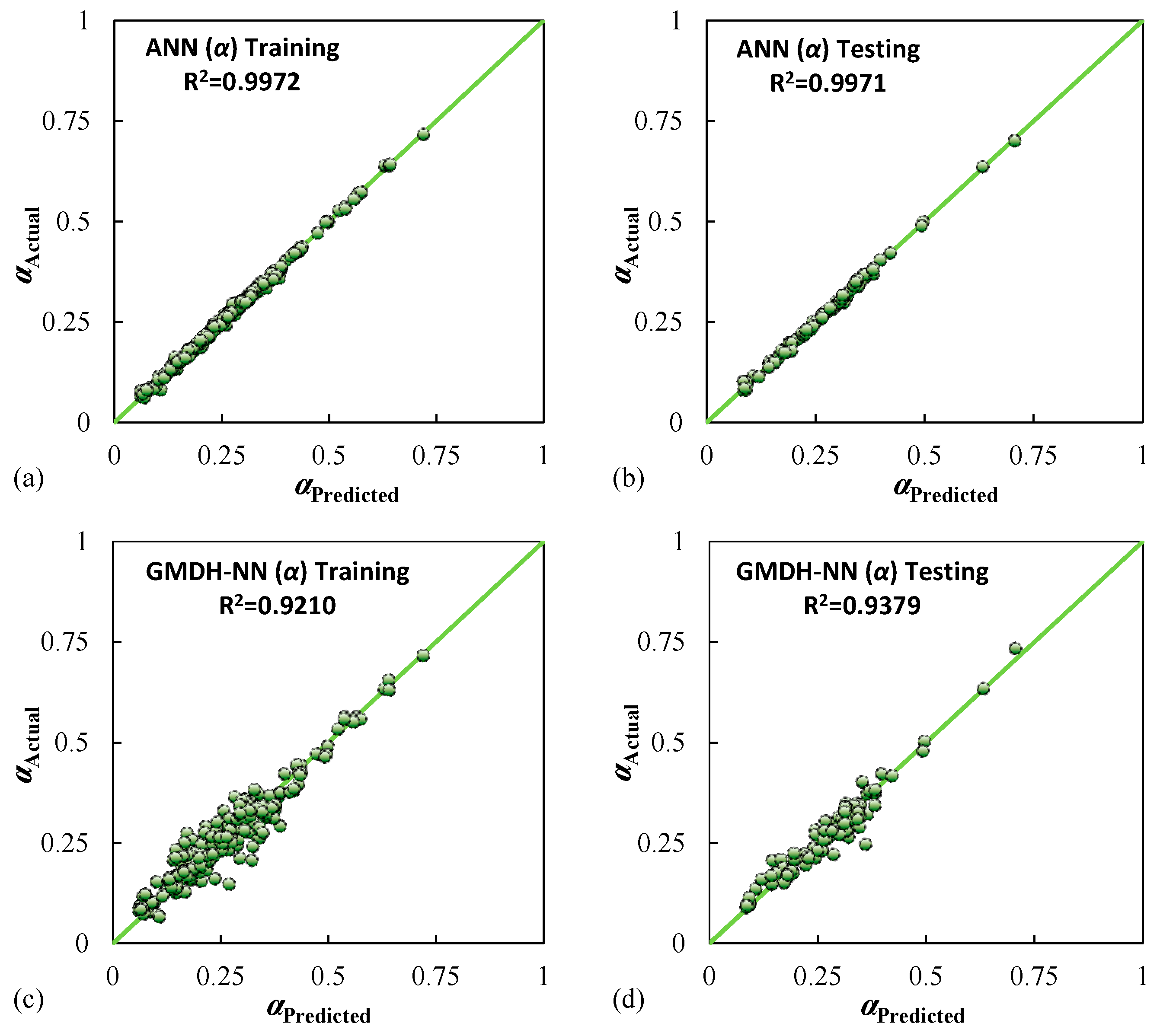
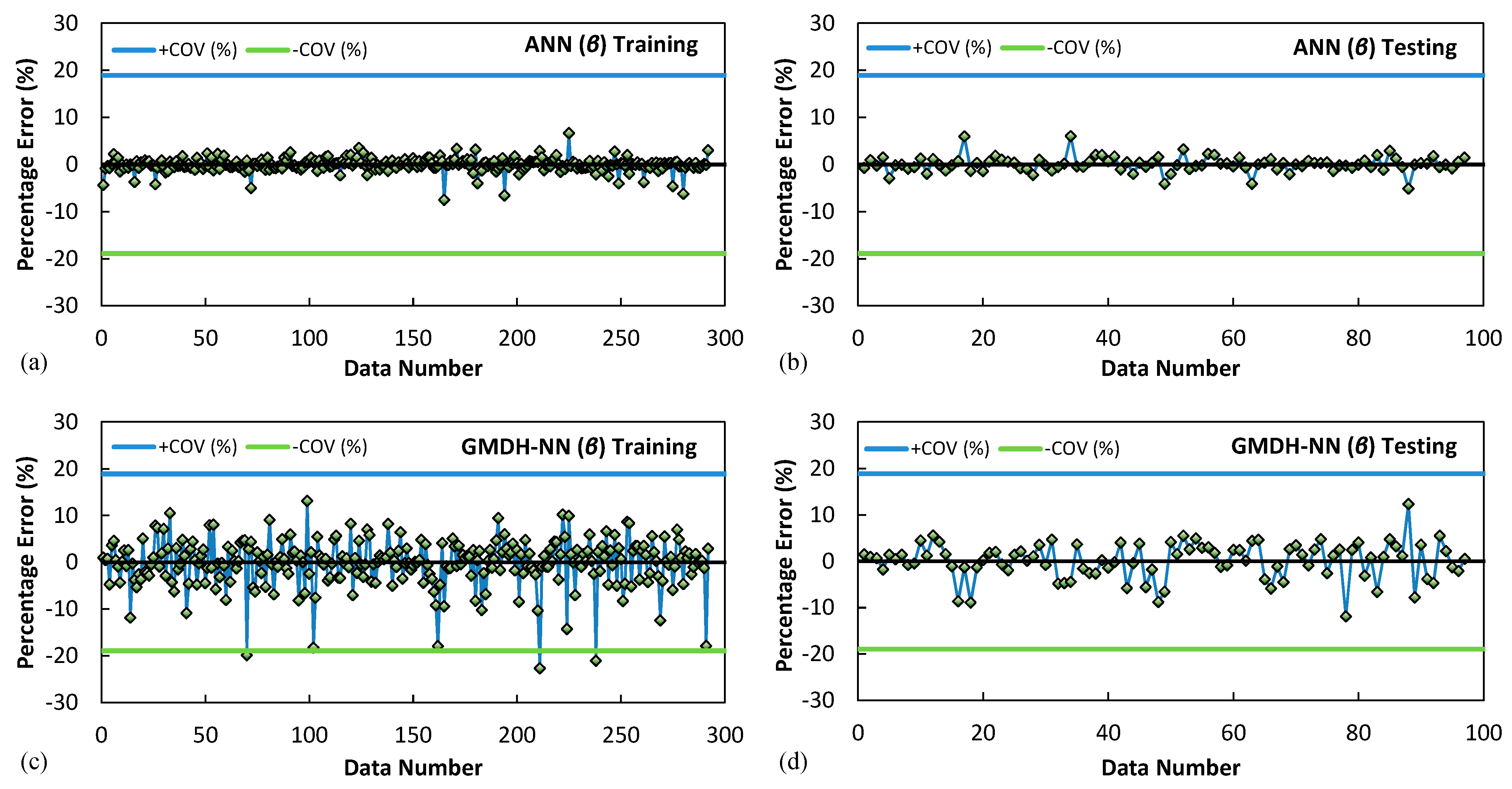
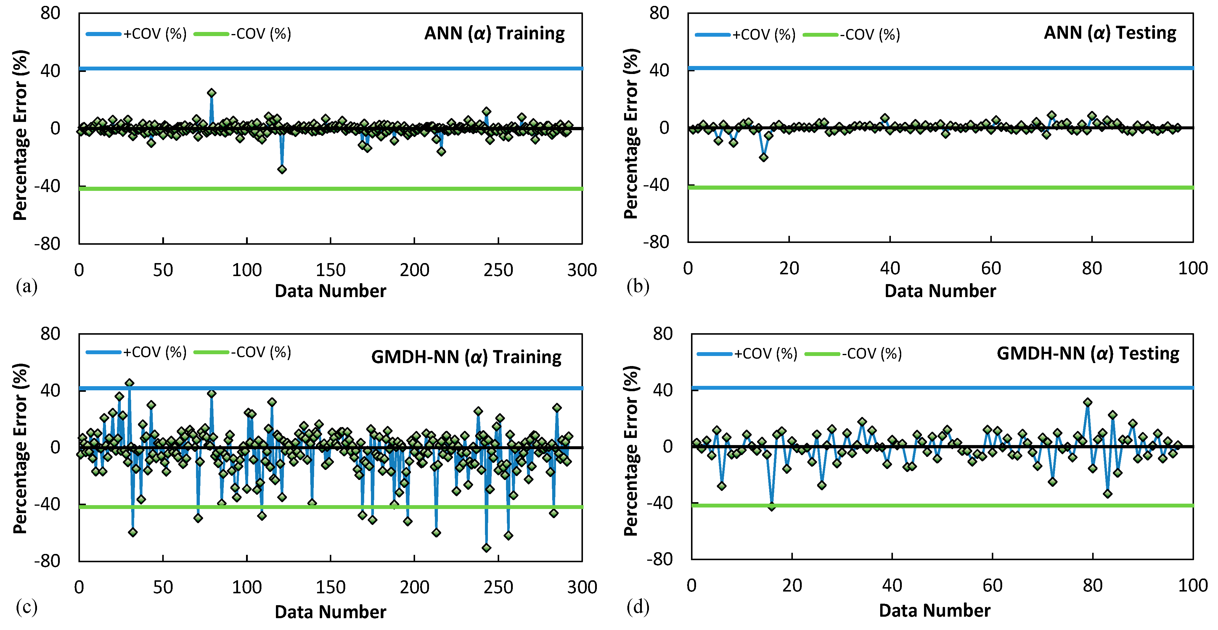
5.5. ML Proposed Models Performances

To evaluate the performance of the ANN and GMDH-NN models, Equations (26)–(31) were used, which are typical criteria for measuring error and model performance [100], including the correlation coefficient (R) and the coefficient of determination (R2), mean square error (MSE), root-mean-square error (RMSE), mean absolute error (MAE) and mean absolute percentage error (MAPE). Detailed results are presented in Table 6 for each developed model.
R = i = 1 n ( A i A ¯ ) ( F i F ¯ ) i = 1 n ( A i A ¯ ) 2 i = 1 n ( F i F ¯ ) 2
R 2 = ( i = 1 n ( A i A ¯ ) ( F i F ¯ ) i = 1 n ( A i A ¯ ) 2 i = 1 n ( F i F ¯ ) 2 ) 2
M S E = 1 n i = 1 n ( A i F i ) 2
R M S E = 1 n i = 1 n ( A i F i ) 2
M A E = 1 n i = 1 n | A i F i |
M A P E = 1 n [ i = 1 n | A i F i | i = 1 n | A i | ] × 100
In Equations (26)–(31), Ai indicates the analysed value, and Fi represents the estimated value, n is the number of the considered data, A ¯ is the mean analysed values, and F ¯ is the mean estimated values.
As shown in Table 6, R and R2 for the ANN models (ANN (β) and ANN (α)) in both training and testing steps are more than the GMDH-NN models (GMDH-NN (β) and GMDH-NN (α)). In the same manner, the evaluated error criteria demonstrate that the ANN models became more accurate than corresponding GMDH-NN models. In particular, the ANN (β) model with R2 values of 0.9949 and 0.9834 and MAPE values of 0.91 and 1.18, respectively, in training and testing stages, outperforms the corresponding GMDH-NN (β) model, with R2 values of 0.9459 and 0.9494 and MAPE values of 3.55 and 3.03, respectively, in training and testing stages. Moreover, regarding the α estimation models, ANN (α) model with R2 values of 0.9972 and 0.9971 and MAPE values of 2.23 and 2.21, respectively, in training and testing stages, outperforms corresponding GMDH-NN (α) model, with R2 values of 0.9210 and 0.9379 and MAPE values of 10.90 and 8.16, respectively, in training and testing stages. The comparison between the measured and predicted values obtained from the ANN and the GMDH models in the training and testing phases for estimating α and β are presented in Figure 17 and Figure 18, respectively.
Figure 17 and Figure 18 indicate that the ANN models produce more accurate and well-fitted ideal fit lines than the GMDH-NN models. Additionally, the error values of β and α proposed models for training and test data stages are presented in Figure 19 and Figure 20, respectively. An acceptable very low error for both proposed ANN and GMDH-NN models could be inferred from Figure 19 and Figure 20.

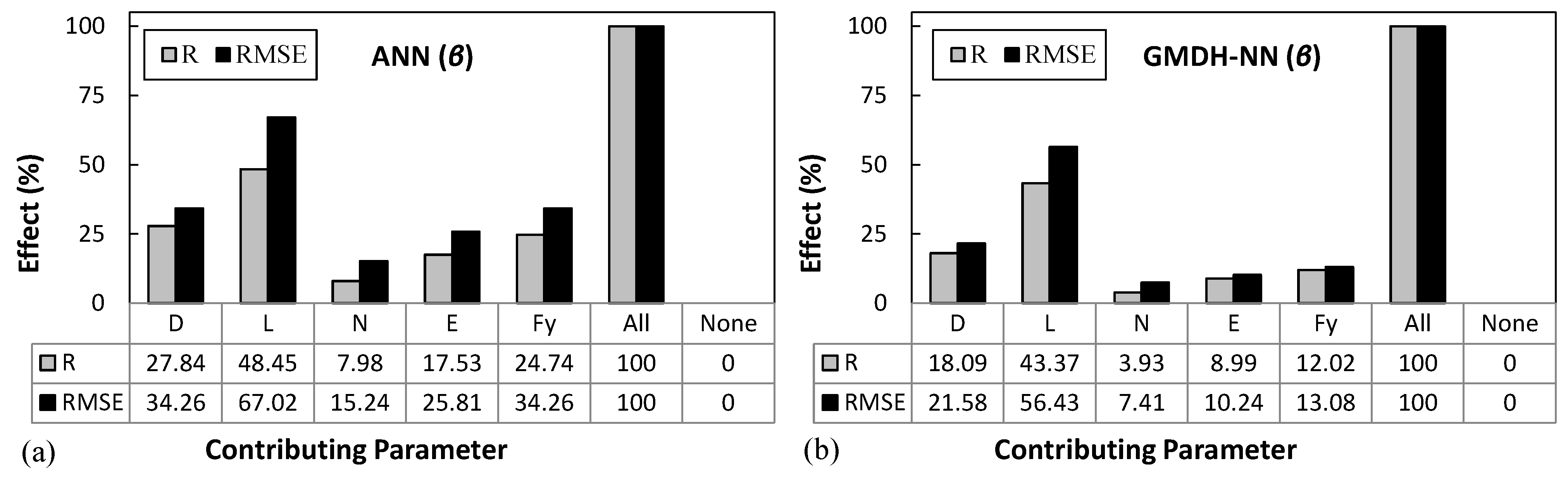
5.6. Sensitivity Analysis

Sensitivity analysis was performed to evaluate the contribution of each input parameter to the ANN and GMDH developed β and α models. Results for each input variable were obtained by assuming that each input variable varies between its minimum and maximum values and that other parameters are maintained at their mean values. Therefore, it was analysed how each parameter affects the correlation coefficient (R) and the root-mean-square error (RMSE). By substituting all or none of the variables with their mean values, the impact on R and RMSE could be considered to be zero and 100%, respectively. The R and RMSE impact may be defined as a percentage value using the following equation [101]:
Effect = [(ZvarZOri) / (ZallZOri)] × 100%
In this equation, ZVar is the R and RMSE values for the considered variable, ZOri is the effect of zero on the R and RMSE, and Zall is equal to the R and RMSE value of the proposed model when all the variables are substituted with their mean values. As shown in Figure 21 and Figure 22, for both β and α, the calculated SMA bars length (L) is the most influential input variable in both ANN and GMDH-NN models. On the other hand, the number of SMA bars (N) has the least effect in both ANN and GMDH-NN models.

5.7. Computational Costs

Various machine learning (ML) techniques could be utilised to estimate the first yield point displacement and post-yield stiffness ratio in SMA-BHDs. However, in this paper, new models were developed by the artificial neural network (ANN) and group method of data handling (GMDH) techniques. The previous sections showed that proposed ANN models outperform GMDH models with lower errors and higher with low errors and high accuracy. On the other hand, considering the computational costs related to ML models’ complexity, it can be mentioned that the proposed GMDH models, with less complex closed-form equations, perform better in comparison with ANN models.

6. Conclusions

A novel bar hysteretic dampers equipped with shape memory alloy (SMA) bars, named SMA-BHDs, as an added damper to isolation systems, was studied in this paper. In order to predict the cyclic behaviour of these dampers, 630 numerical models including different geometrical and mechanical properties were constructed in SeismoStruct software. The obtained hysteretic curves from numerical models were idealised by bilinear curves to achieve pre- and post-yield parameters such as the first yield point displacement (Dy), elastic stiffness (Ke), and post-yield stiffness ration (α). The analyses show that the existing analytical equation for determining Dy is not consistent with obtained results from hysteretic curves and needs modification. Moreover, there is no analytical equation for estimating the α parameter. Therefore, two machine learning approaches, named artificial neural network (ANN) and group method of data handling integrated by a neural network (GMDH-NN), were utilised to estimate the Dy modification factor (β) and propose an equation for α parameter for the first time. An overview of the results of this paper is presented as follows:
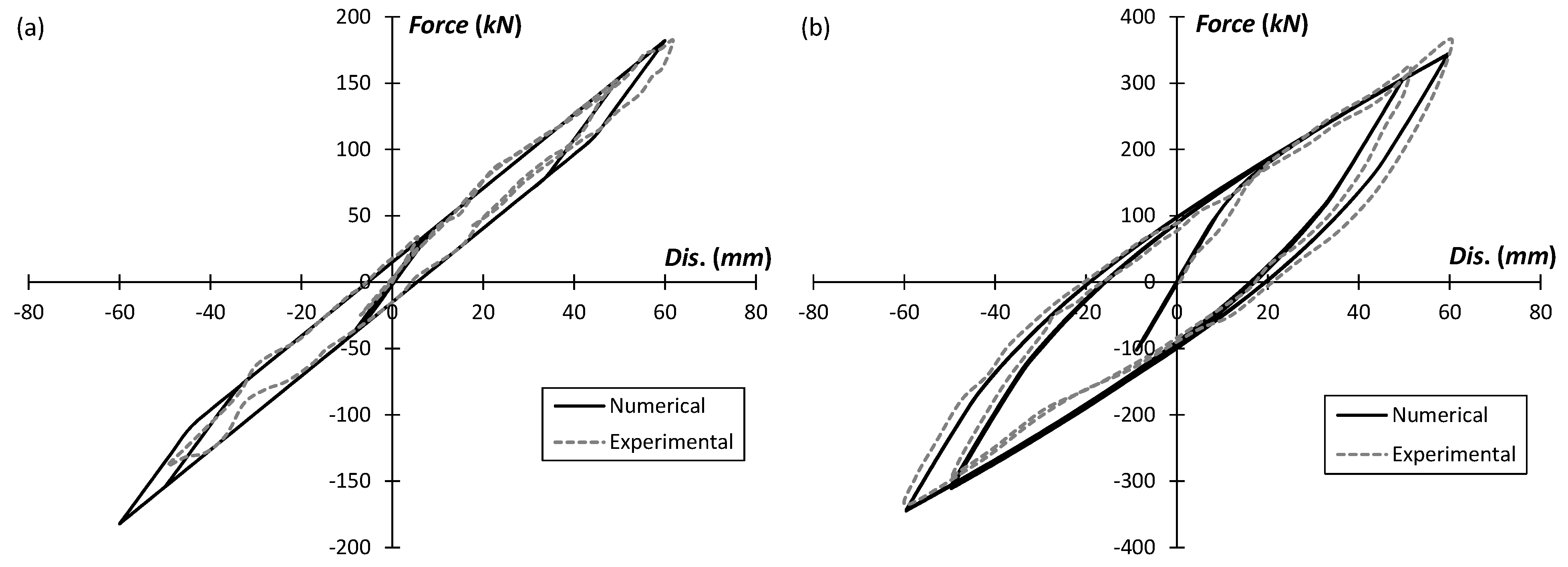
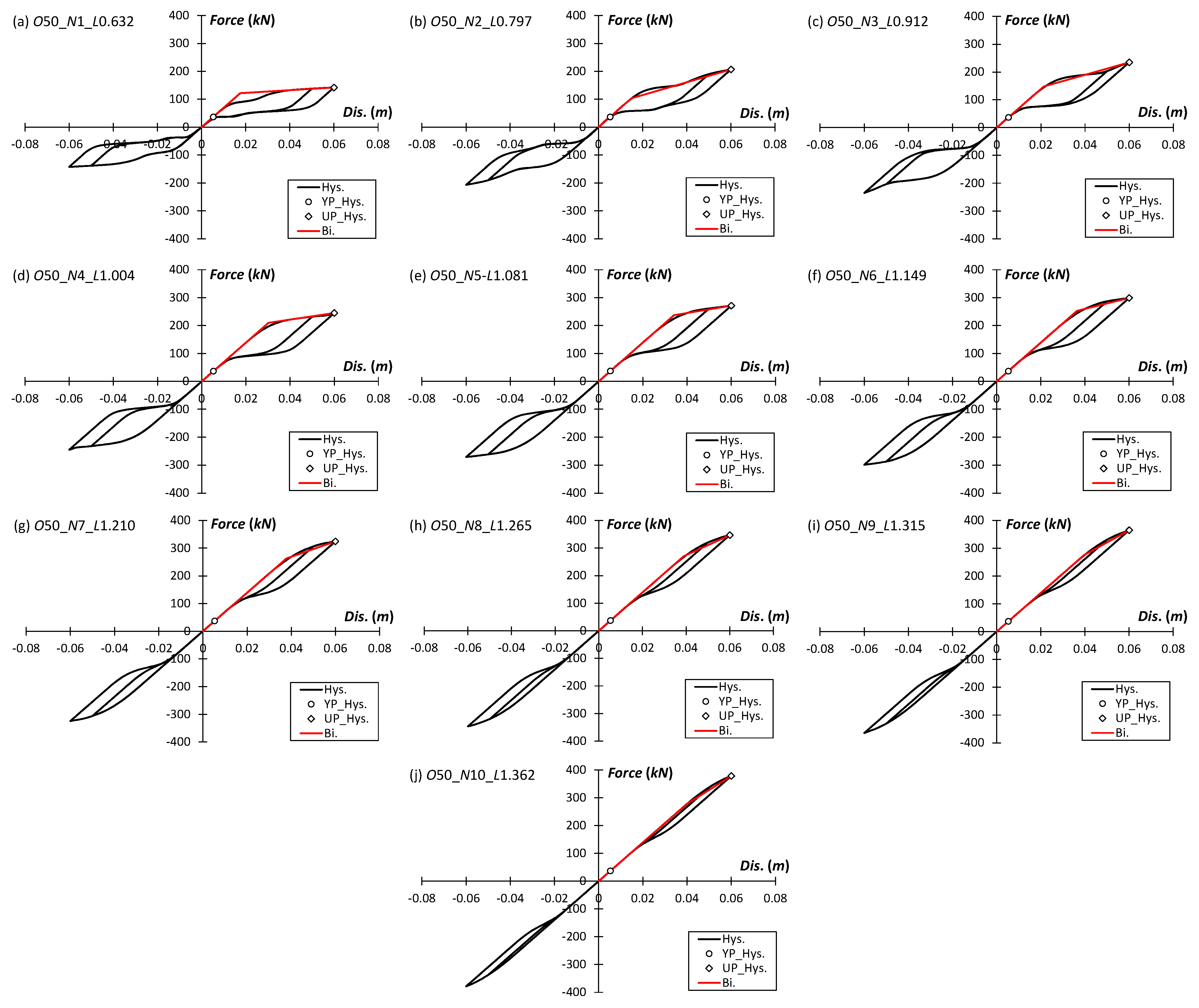
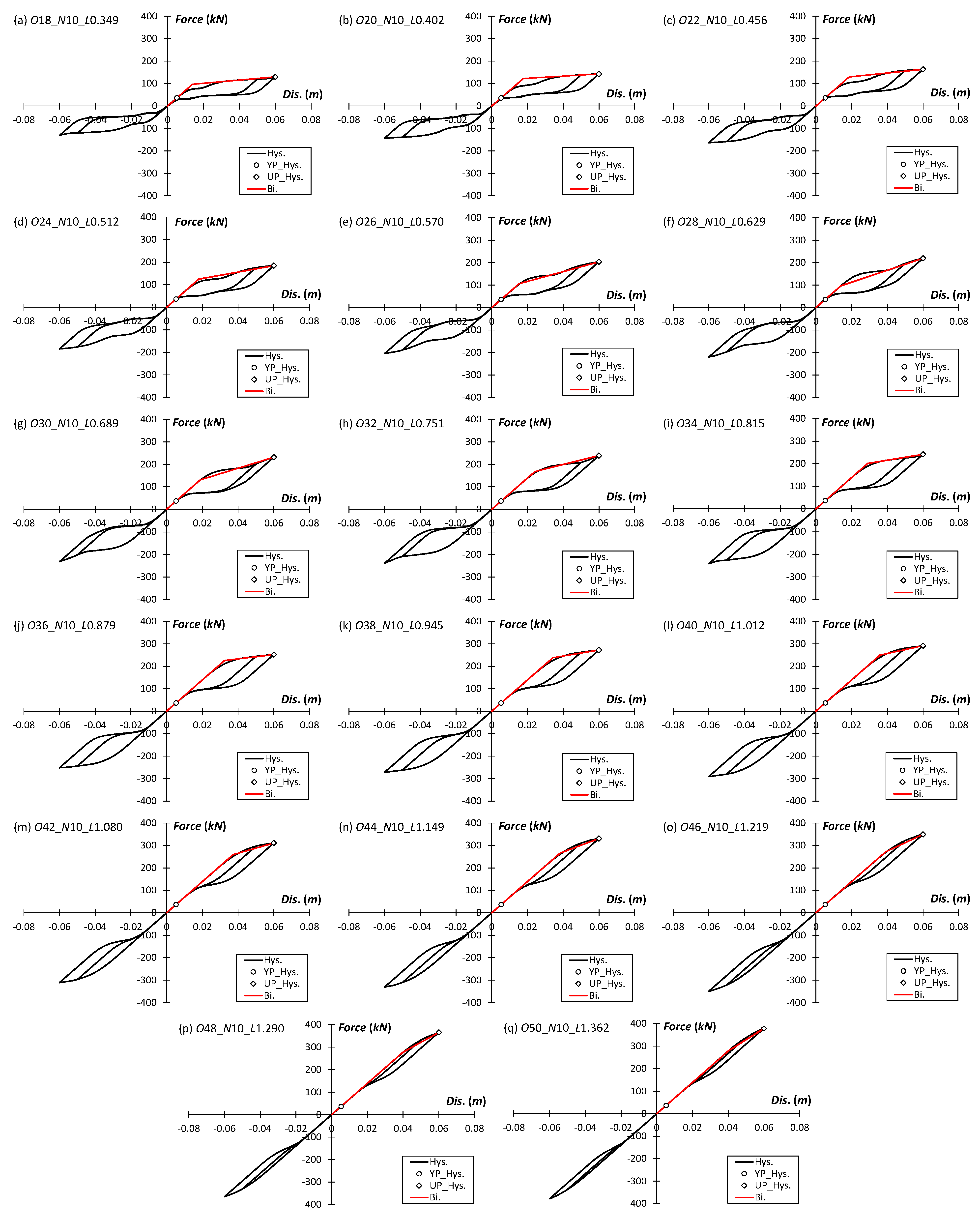
  • As expected, by substituting SMA bars instead of steel bar in bar hysteretic dampers, no residual displacement could be seen in hysteretic curves, which shows the excellent performance of SMA-BHDs as added dampers to isolation systems.
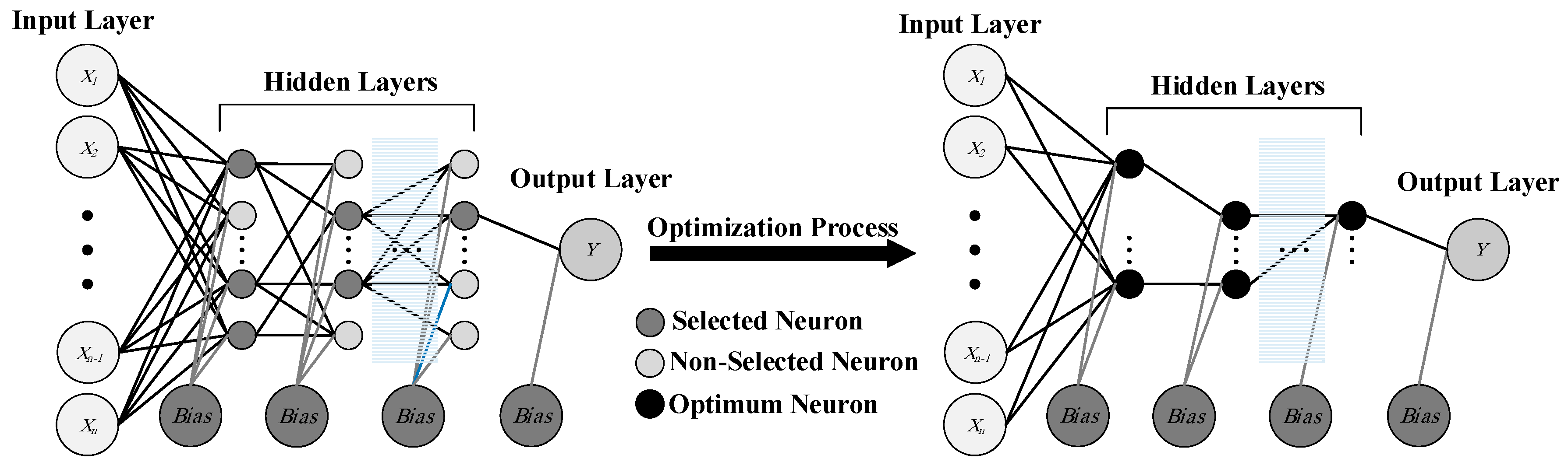
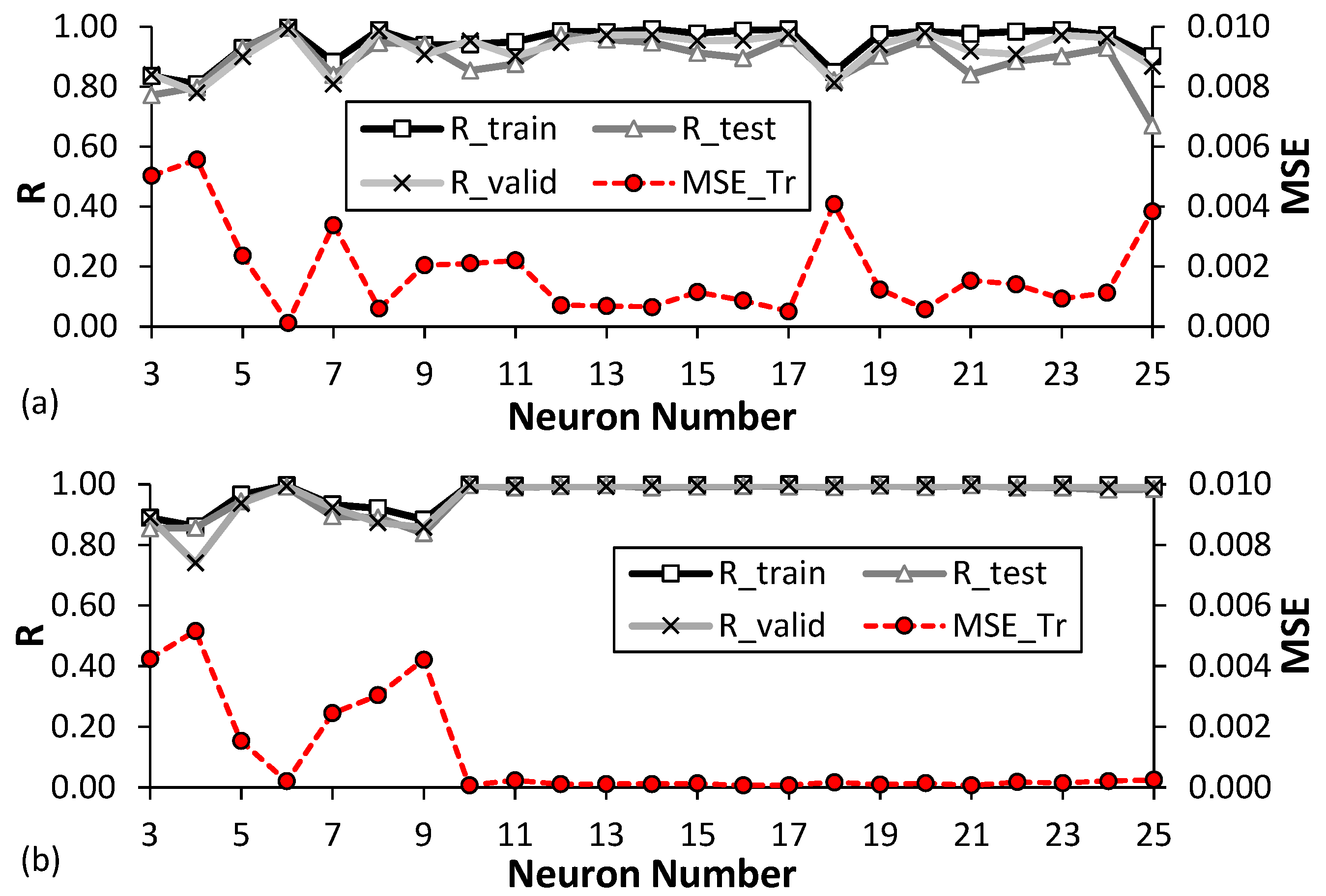
  • Considering the ANN models with one hidden layer and varying neuron numbers between 3 to 25, the neural networks with 10 and 6 hidden neurons were selected as the optimised network structure for β and α parameters, respectively. The ANN (β) model has the R values of 0.9972, 0.9958, and 0.9916 in training, testing, and validation data sets and considerably small MSE values of 0.00012 and 0.00047, and MAPE values of 2.60% and 3.31%, in training and testing data sets, respectively. On the other hand, ANN (α) model has the R values of 0.9986, 0.9966, and 0.9972 in training, testing, and validation data sets and MSE values of 0.00007 and 0.00008, and MAPE values of 2.34% and 2.43%, in training and testing data sets, respectively.
  • In the GMDH-NN models, similarly to ANN models, around 25% of all databases (97 data from 389 data) were randomly set aside for the test stage and considered unseen data. The results show that the proposed ANN models with higher R2 and lower error values in both the training and testing stages outperform the proposed GMDH-NN models. However, compared with the ANN model, GMDH-NN models present more user-friendly and easy-to-interpret closed-form equations.
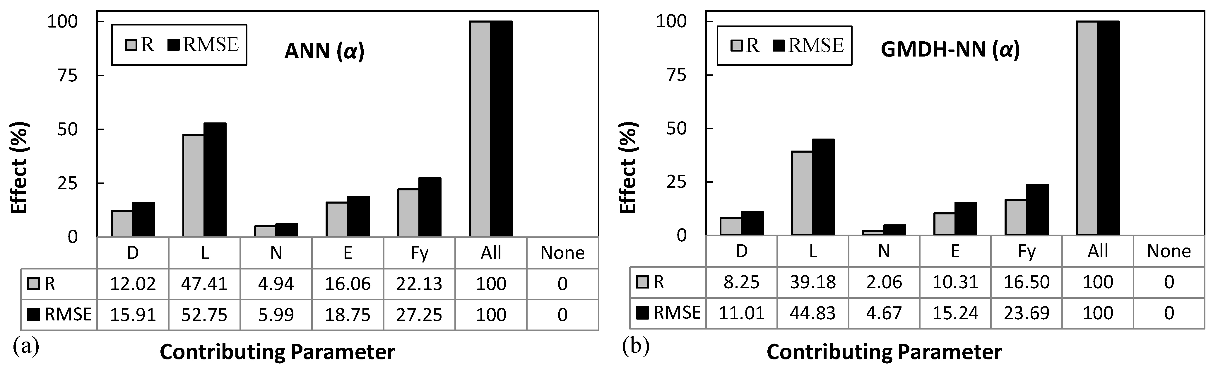
  • The sensitivity analysis of the input parameters in the developed ANN and GMDH-NN models for estimating both β and α parameters showed that the calculated SMA bars length (L) variable with higher R and RMSE values is the most influential input variable. Furthermore, the number of SMA bars (N) with lower impact values on the R and RMSE has the least effect.

Author Contributions

Conceptualisation, H.J., D.R.E. and M.K.; methodology, D.R.E., H.J. and M.K.; software, S.A.N.J., H.J. and D.R.E.; validation, D.R.E., H.J. and A.K.; formal analysis, D.R.E., H.J., V.F. and A.K.; investigation, H.H., M.K., S.A.N.J. and V.F.; resources, H.J., D.R.E., A.K. and N.F.; data curation, D.R.E. and H.J.; writing—original draft preparation, H.J., A.K., H.H. and S.A.N.J.; writing—review and editing, H.J., D.R.E., V.F., N.F. and M.K.; visualisation, H.J., D.R.E., H.H. and N.F.; supervision, H.J., D.R.E. and M.K.; project administration, H.J., D.R.E. and M.K.; funding acquisition, V.F. and M.K. All authors have read and agreed to the published version of the manuscript.

Funding

This research received no external funding.

Institutional Review Board Statement

Not applicable.

Informed Consent Statement

Not applicable.

Data Availability Statement

The data presented in this study are available on request from the corresponding author. The data are not publicly available due to privacy restrictions.

Conflicts of Interest

The authors declare no conflict of interest.

References

  1. Jahangir, H.; Khatibinia, M.; Kavousi, M. Application of Contourlet Transform in Damage Localization and Severity Assessment of Prestressed Concrete Slabs. Soft Comput. Civ. Eng. 2021, 5, 39–67. [Google Scholar] [CrossRef]
  2. Santandrea, M.; Imohamed, I.A.O.; Jahangir, H.; Carloni, C.; Mazzotti, C.; De Miranda, S.; Ubertini, F.; Casadei, P. An investigation of the debonding mechanism in steel FRP-and FRCM-concrete joints. In Proceedings of the 4th Workshop on The New Boundaries of Structural Concrete, Capri Island, Italy, 29 September–1 October 2016; pp. 289–298. [Google Scholar]
  3. Karimipour, A.; Ghalehnovi, M. Influence of steel fibres on the mechanical and physical performance of self-compacting concrete manufactured with waste materials and fillers. Constr. Build. Mater. 2021, 267, 121806. [Google Scholar] [CrossRef]
  4. Ghalehnovi, M.; Karimipour, A.; Anvari, A.; de Brito, J. Flexural strength enhancement of recycled aggregate concrete beams with steel fibre-reinforced concrete jacket. Eng. Struct. 2021, 240, 112325. [Google Scholar] [CrossRef]
  5. Jahangir, H.; Karamodin, A. Structural Behavior Investigation Based on Adaptive Pushover Procedure. In Proceedings of the 10th National Congress on Civil Engineering, Tehran, Iran, 27–29 December 2015. [Google Scholar]
  6. Khaleghi, M.; Salimi, J.; Farhangi, V.; Moradi, M.J.; Karakouzian, M. Application of Artificial Neural Network to Predict Load Bearing Capacity and Stiffness of Perforated Masonry Walls. CivilEng 2021, 2, 4. [Google Scholar] [CrossRef]
  7. Hasani, H.; Ryan, K.L. Experimental Cyclic Test of Reduced Damage Detailed Drywall Partition Walls Integrated with a Timber Rocking Wall. J. Earthq. Eng. 2021, 1, 1–21. [Google Scholar] [CrossRef]
  8. Jahangir, H.; Esfahani, M.R. Structural Damage Identification Based on Modal Data and Wavelet Analysis. In Proceedings of the 3rd National Conference on Earthquake & Structure, Kerman, Iran, 17–18 October 2012. [Google Scholar]
  9. Jahangir, H.; Esfahani, M.R. Damage localization of Structures Using Adaptive Neuro-Fuzzy Inference System. In Proceedings of the 7th National Congress on Civil Engineering, Zahedan, Iran, 7 May 2013. [Google Scholar]
  10. Seyedi, S.R.; Keyhani, A.; Jahangir, H. An Energy-Based Damage Detection Algorithm Based on Modal Data. In Proceedings of the 7th International Conference on Seismologhy and Earthquake Engineering, International Institute of Earthquake Engineering and Seismology (IIEES), Tehran, Iran, 17–20 May 2015; pp. 335–336. [Google Scholar]
  11. Soong, T.; Dargush, G. Passive Energy Dissipation Systems in Structural Engineering; John Wiley Sons: London, UK, 1997. [Google Scholar]
  12. Castaldo, P. Integrated Seismic Design of Structure and Control Systems; Springer Tracts in Mechanical Engineering; Springer International Publishing: Cham, Switzerland, 2014; ISBN 978-3-319-02614-5. [Google Scholar]
  13. Michalski, R.S.; Carbonell, J.G.; Mitchell, T.M. Machine Learning: An Artificial Intelligence Approach; Springer Science & Business Media: Berlin, Germany, 2013. [Google Scholar]
  14. Chen, Y.; Yan, J.; Feng, J.; Sareh, P. Particle Swarm Optimization-Based Metaheuristic Design Generation of Non-Trivial Flat-Foldable Origami Tessellations with Degree-4 Vertices. J. Mech. Des. 2021, 143, 011703. [Google Scholar] [CrossRef]
  15. Fan, W.; Chen, Y.; Li, J.; Sun, Y.; Feng, J.; Hassanin, H.; Sareh, P. Machine learning applied to the design and inspection of reinforced concrete bridges: Resilient methods and emerging applications. Structures 2021, 33, 3954–3963. [Google Scholar] [CrossRef]
  16. Di Cesare, A.; Ponzo, F.C.; Nigro, D. Assessment of the performance of hysteretic energy dissipation bracing systems. Bull. Earthq. Eng. 2014, 12, 2777–2796. [Google Scholar] [CrossRef]
  17. Javanmardi, A.; Ibrahim, Z.; Ghaedi, K.; Benisi Ghadim, H.; Hanif, M.U. State-of-the-Art Review of Metallic Dampers: Testing, Development and Implementation. Arch. Comput. Methods Eng. 2019, 27, 455–478. [Google Scholar] [CrossRef]
  18. Guerrero, J. Bandas amortiguadoras para muros de partición (damping strips for partition walls). In Proceedings of the Primer Congreso Nacional de Ingenieria Sısmica, Guadalajara, Mexico, 17 May 1965; pp. 75–85. [Google Scholar]
  19. Muto, K. Earthquake resistant design of 36-storied Kasumigaseki building. In Proceedings of the 4th World Conference of Earthquake Engineering, Santiago de, Chile, Chile, 13–18 January 1969; pp. 16–33. [Google Scholar]
  20. Kelly, J.M.; Skinner, R.I.; Heine, A.J. Mechanisms of energy absorption in special devices for use in earthquake resistant structures. Bull. N.Z. Soc. Earthq. Eng. 1972, 5, 63–88. [Google Scholar]
  21. Skinner, R.I.; Kelly, J.M.; Heine, A.J. Hysteretic dampers for earthquake-resistant structures. Earthq. Eng. Struct. Dyn. 1974, 3, 287–296. [Google Scholar] [CrossRef]
  22. Bergman, D.; Goel, S. Evaluation of Cyclic Testing of Steel-Plate Devices for Added Damping and Stifness; Department of Civil Engineering, University of Michigan: Michigan, MI, USA, 1987. [Google Scholar]
  23. Tsai, K.; Chen, H.; Hong, C.; Su, Y. Design of Steel Triangular Plate Energy Absorbers for Seismic-Resistant Construction. Earthq. Spectra 1993, 9, 505–528. [Google Scholar] [CrossRef]
  24. Tehranizadeh, M. Passive energy dissipation device for typical steel frame building in Iran. Eng. Struct. 2001, 23, 643–655. [Google Scholar] [CrossRef]
  25. Bakre, S.V.; Jangid, R.S.; Reddy, G.R. Optimum X-plate dampers for seismic response control of piping systems. Int. J. Press. Vessel. Pip. 2006, 83, 672–685. [Google Scholar] [CrossRef]
  26. Ming-Hsiang, S.; Wen-pei, S.; Cheer-Germ, G.O. Investigation of newly developed added damping and stiffness device with low yield strength steel. J. Zhejiang Univ. A 2004, 5, 326–334. [Google Scholar] [CrossRef]
  27. Shih, M.-H.; Sung, W.-P. A model for hysteretic behavior of rhombic low yield strength steel added damping and stiffness. Comput. Struct. 2005, 83, 895–908. [Google Scholar] [CrossRef]
  28. Han, Q.; Jia, J.; Xu, Z.; Bai, Y.; Song, N. Experimental Evaluation of Hysteretic Behavior of Rhombic Steel Plate Dampers. Adv. Mech. Eng. 2014, 6, 185629. [Google Scholar] [CrossRef]
  29. Chan, R.W.K.; Albermani, F. Experimental study of steel slit damper for passive energy dissipation. Eng. Struct. 2008, 30, 1058–1066. [Google Scholar] [CrossRef]
  30. Lee, C.-H.; Kim, J.; Kim, D.-H.; Ryu, J.; Ju, Y.K. Numerical and experimental analysis of combined behavior of shear-type friction damper and non-uniform strip damper for multi-level seismic protection. Eng. Struct. 2016, 114, 75–92. [Google Scholar] [CrossRef]
  31. Lee, J.; Kim, J. Development of box-shaped steel slit dampers for seismic retrofit of building structures. Eng. Struct. 2017, 150, 934–946. [Google Scholar] [CrossRef]
  32. Ahmadie Amiri, H.; Najafabadi, E.P.; Estekanchi, H.E. Experimental and analytical study of Block Slit Damper. J. Constr. Steel Res. 2018, 141, 167–178. [Google Scholar] [CrossRef]
  33. Köroğlu, M.A.; Köken, A.; Dere, Y. Use of different shaped steel slit dampers in beam to column connections of steel frames under cycling loading. Adv. Steel Constr. 2018, 14, 251–273. [Google Scholar]
  34. Jahangir, H.; Daneshvar Khorram, M.H.; Ghalehnovi, M. Influence of Geometric Parameters on Perforated Core Buckling Restrained Braces Behavior. J. Struct. Constr. Eng. 2018, 6, 75–94. (In Persian) [Google Scholar] [CrossRef]
  35. Bayat, K.; Shekastehband, B. Seismic performance of beam to column connections with T-shaped slit dampers. Thin-Walled Struct. 2019, 141, 28–46. [Google Scholar] [CrossRef]
  36. Liu, Y.; Aoki, T.; Shimoda, M. Strain Distribution Measurement of a Shear Panel Damper Developed for Bridge Structure. J. Struct. 2013, 2013, 1–11. [Google Scholar] [CrossRef]
  37. Deng, K.; Pan, P.; Sun, J.; Liu, J.; Xue, Y. Shape optimization design of steel shear panel dampers. J. Constr. Steel Res. 2014, 99, 187–193. [Google Scholar] [CrossRef]
  38. Sahoo, D.R.; Singhal, T.; Taraithia, S.S.; Saini, A. Cyclic behavior of shear-and-flexural yielding metallic dampers. J. Constr. Steel Res. 2015, 114, 247–257. [Google Scholar] [CrossRef]
  39. Deng, K.; Pan, P.; Li, W.; Xue, Y. Development of a buckling restrained shear panel damper. J. Constr. Steel Res. 2015, 106, 311–321. [Google Scholar] [CrossRef]
  40. Taherian, I.; Ghalehnovi, M.; Jahangir, H. Analytical Study on Composite Steel Plate Walls Using a Modified Strip Model. In Proceedings of the 7th International Conference on Seismologhy and Earthquake Engineering, Tehran, Iran, 17–20 May 2015. [Google Scholar]
  41. Qiu, C.; Zhang, Y.; Qu, B.; Dai, C.; Hou, H.; Li, H. Cyclic testing of seismic dampers consisting of multiple energy absorbing steel plate clusters. Eng. Struct. 2019, 183, 255–264. [Google Scholar] [CrossRef]
  42. Garivani, S.; Aghakouchak, A.A.; Shahbeyk, S. Numerical and experimental study of comb-teeth metallic yielding dampers. Int. J. Steel Struct. 2016, 16, 177–196. [Google Scholar] [CrossRef]
  43. Ciampi, V. Research and development of passive energy dissipation techniques for civil buildings in Italy. In Proceedings of the International Post—SMIRT Conference Seminar on Seismic Isolation, Passiver Energy Dissipation and Control of Vibration of Structures, Milan, Italy, 5 May 1995; pp. 1–15. [Google Scholar]
  44. Kato, S.; Kim, Y.-B.; Nakazawa, S.; Ohya, T. Simulation of the cyclic behavior of J-shaped steel hysteresis devices and study on the efficiency for reducing earthquake responses of space structures. J. Constr. Steel Res. 2005, 61, 1457–1473. [Google Scholar] [CrossRef]
  45. Kato, S.; Kim, Y.-B. A finite element parametric study on the mechanical properties of J-shaped steel hysteresis devices. J. Constr. Steel Res. 2006, 62, 802–811. [Google Scholar] [CrossRef]
  46. Oh, S.-H.; Song, S.-H.; Lee, S.-H.; Kim, H.-J. Seismic response of base isolating systems with U-shaped hysteretic dampers. Int. J. Steel Struct. 2012, 12, 285–298. [Google Scholar] [CrossRef]
  47. Deng, K.; Pan, P.; Wang, C. Development of crawler steel damper for bridges. J. Constr. Steel Res. 2013, 85, 140–150. [Google Scholar] [CrossRef]
  48. Maoshe, L.I.U.; Junlong, L.U. Analysis of Shear Stiffness of the Thin U-Shape Metal Damper [J]. J. Xi’an Univ. Technol. 2013, 29, 207–210. [Google Scholar]
  49. Deng, K.; Pan, P.; Su, Y.; Xue, Y. Shape optimization of U-shaped damper for improving its bi-directional performance under cyclic loading. Eng. Struct. 2015, 93, 27–35. [Google Scholar] [CrossRef]
  50. Bagheri, S.; Barghian, M.; Saieri, F.; Farzinfar, A. U-shaped metallic-yielding damper in building structures: Seismic behavior and comparison with a friction damper. Structures 2015, 3, 163–171. [Google Scholar] [CrossRef]
  51. Ene, D.; Kishiki, S.; Yamada, S.; Jiao, Y.; Konishi, Y.; Terashima, M.; Kawamura, N. Experimental study on the bidirectional inelastic deformation capacity of U-shaped steel dampers for seismic isolated buildings. Earthq. Eng. Struct. Dyn. 2016, 45, 173–192. [Google Scholar] [CrossRef]
  52. Wang, B.; Zhu, S. Superelastic SMA U-shaped dampers with self-centering functions. Smart Mater. Struct. 2018, 27, 055003. [Google Scholar] [CrossRef]
  53. Taiyari, F.; Mazzolani, F.M.; Bagheri, S. A proposal for energy dissipative braces with U-shaped steel strips. J. Constr. Steel Res. 2019, 154, 110–122. [Google Scholar] [CrossRef]
  54. Ghaedi, K.; Ibrahim, Z.; Javanmardi, A.; Rupakhety, R. Experimental Study of a New Bar Damper Device for Vibration Control of Structures Subjected to Earthquake Loads. J. Earthq. Eng. 2018, 25, 1–19. [Google Scholar] [CrossRef]
  55. Ghaedi, K.; Ibrahim, Z.; Javanmardi, A. A new metallic bar damper device for seismic energy dissipation of civil structures. IOP Conf. Ser. Mater. Sci. Eng. 2018, 431, 122009. [Google Scholar] [CrossRef]
  56. Aghlara, R.; Tahir, M.M. A passive metallic damper with replaceable steel bar components for earthquake protection of structures. Eng. Struct. 2018, 159, 185–197. [Google Scholar] [CrossRef]
  57. Golzan, S.B.; Langlois, S.; Legeron, F.P. Implementation of a Simplified Method in Design of Hysteretic Dampers for Isolated Highway Bridges. J. Bridg. Eng. 2017, 22, 04016127. [Google Scholar] [CrossRef]
  58. Jahangir, H.; Bagheri, M.; Delavari, S.M.J. Cyclic Behavior Assessment of Steel Bar Hysteretic Dampers Using Multiple Nonlinear Regression Approach. Iran. J. Sci. Technol. Trans. Civ. Eng. 2021, 45, 1227–1251. [Google Scholar] [CrossRef]
  59. Jahangir, H.; Esfahani, M.R. Numerical Study of Bond–Slip Mechanism in Advanced Externally Bonded Strengthening Composites. KSCE J. Civ. Eng. 2018, 22, 4509–4518. [Google Scholar] [CrossRef]
  60. Bagheri, M.; Chahkandi, A.; Jahangir, H. Seismic Reliability Analysis of RC Frames Rehabilitated by Glass Fiber-Reinforced Polymers. Int. J. Civ. Eng. 2019, 17, 1785–1797. [Google Scholar] [CrossRef]
  61. Jahangir, H.; Esfahani, M.R. Investigating loading rate and fibre densities influence on SRG—Concrete bond behaviour. Steel Compos. Struct. 2020, 34, 877–889. [Google Scholar] [CrossRef]
  62. Jahangir, H.; Esfahani, M.R. Experimental analysis on tensile strengthening properties of steel and glass fiber reinforced inorganic matrix composites. Sci. Iran. 2020, 28, 1152–1166. [Google Scholar] [CrossRef]
  63. Jahangir, H.; Esfahani, M.R. Strain of Newly–Developed Composites Relationship in Flexural Tests. J. Struct. Constr. Eng. 2018, 5, 92–107. (In Persian) [Google Scholar] [CrossRef]
  64. Gebretsadik, B.; Jadidi, K.; Farhangi, V.; Karakouzian, M. Application of Ultrasonic Measurements for the Evaluation of Steel Fiber Reinforced Concrete. Eng. Technol. Appl. Sci. Res. 2021, 11, 6662–6667. [Google Scholar] [CrossRef]
  65. Asgarian, B.; Moradi, S. Seismic response of steel braced frames with shape memory alloy braces. J. Constr. Steel Res. 2011, 67, 65–74. [Google Scholar] [CrossRef]
  66. Dolce, M.; Cardone, D.; Ponzo, F.C. Shaking-table tests on reinforced concrete frames with different isolation systems. Earthq. Eng. Struct. Dyn. 2007, 36, 573–596. [Google Scholar] [CrossRef]
  67. Andrawes, B.; DesRoches, R. Unseating prevention for multiple frame bridges using superelastic devices. Smart Mater. Struct. 2005, 14, S60–S67. [Google Scholar] [CrossRef]
  68. Farhangi, V.; Karakouzian, M. Design of bridge foundations using reinforced micropiles. In Proceedings of the IRF Global Road2Tunnel Conference & Expo, Las Vegas, NV, USA, 19–22 November 2019. [Google Scholar]
  69. Malakooti, A.; Maguire, M.; Thomas, R.J. Evaluating Electrical Resistivity as a Performance Based Test for Utah Bridge Deck Concrete (CAIT-UTC-NC35); Rutgers University, Center for Advanced Infrastructure and Transportation: Piscataway, NJ, USA, 2018. [Google Scholar]
  70. Song, G.; Ma, N.; Li, H.-N. Applications of shape memory alloys in civil structures. Eng. Struct. 2006, 28, 1266–1274. [Google Scholar] [CrossRef]
  71. Farahi, B.; Esfahani, M.; Sabzi, J. Experimental investigation on the behavior of reinforced concrete beams retrofitted with NSM-SMA/FRP. Amirkabir J. Civ. Eng. 2019, 51, 685–698. [Google Scholar] [CrossRef]
  72. Jahangir, H.; Bagheri, M. Evaluation of Seismic Response of Concrete Structures Reinforced by Shape Memory Alloys (Technical Note). Int. J. Eng. 2020, 33. [Google Scholar] [CrossRef]
  73. Karimipour, A.; Edalati, M. Shear and flexural performance of low, normal and high-strength concrete beams reinforced with longitudinal SMA, GFRP and steel rebars. Eng. Struct. 2020, 221, 111086. [Google Scholar] [CrossRef]
  74. Sabzi, J.; Esfahani, M.R.; Ozbakkaloglu, T.; Farahi, B. Effect of concrete strength and longitudinal reinforcement arrangement on the performance of reinforced concrete beams strengthened using EBR and EBROG methods. Eng. Struct. 2020, 205, 110072. [Google Scholar] [CrossRef]
  75. Jalali, A.; Cardone, D.; Narjabadifam, P. Smart restorable sliding base isolation system. Bull. Earthq. Eng. 2011, 9, 657–673. [Google Scholar] [CrossRef]
  76. Zafar, A.; Andrawes, B. Incremental dynamic analysis of concrete moment resisting frames reinforced with shape memory composite bars. Smart Mater. Struct. 2012, 21, 025013. [Google Scholar] [CrossRef]
  77. Alam, M.S.; Youssef, M.A.; Nehdi, M.L. Exploratory investigation on mechanical anchors for connecting SMA bars to steel or FRP bars. Mater. Struct. 2010, 43, 91–107. [Google Scholar] [CrossRef]
  78. Shrestha, B.; Li, C.; Hao, H.; Li, H. Performance-Based Seismic Assessment of Superelastic Shape Memory Alloy-Reinforced Bridge Piers Considering Residual Deformations. J. Earthq. Eng. 2017, 21, 1050–1069. [Google Scholar] [CrossRef]
  79. DesRoches, R.; McCormick, J.; Delemont, M. Cyclic Properties of Superelastic Shape Memory Alloy Wires and Bars. J. Struct. Eng. 2004, 130, 38–46. [Google Scholar] [CrossRef]
  80. Malécot, P.; Lexcellent, C.; Folte^te, E.; Collet, M. Shape Memory Alloys Cyclic Behavior: Experimental Study and Modeling. J. Eng. Mater. Technol. 2006, 128, 335–345. [Google Scholar] [CrossRef]
  81. Auricchio, F.; Sacco, E. A Superelastic Shape-Memory-Alloy Beam Model. J. Intell. Mater. Syst. Struct. 1997, 8, 489–501. [Google Scholar] [CrossRef]
  82. Seismosoft. Seismostruct V7.0—A Computer Program for Static and Dynamic Nonlinear Analysis of Framed Structures; Seismic Support, Inc.: Pavia, Italy, 2014. [Google Scholar]
  83. Roshani, M.M.; Kargar, S.H.; Farhangi, V.; Karakouzian, M. Predicting the effect of fly ash on concrete’s mechanical properties by ann. Sustainibility 2021, 13, 1469. [Google Scholar] [CrossRef]
  84. Ghaderi, A.; Morovati, V.; Dargazany, R. A physics-informed assembly of feed-forward neural network engines to predict inelasticity in cross-linked polymers. Polymers 2020, 12, 2628. [Google Scholar] [CrossRef]
  85. Rezazadeh Eidgahee, D.; Rafiean, A.H.; Haddad, A. A Novel Formulation for the Compressive Strength of IBP-Based Geopolymer Stabilized Clayey Soils Using ANN and GMDH-NN Approaches. Iran. J. Sci. Technol. Trans. Civ. Eng. 2019, 44, 219–229. [Google Scholar] [CrossRef]
  86. Moradi, M.J.; Khaleghi, M.; Salimi, J.; Farhangi, V.; Ramezanianpour, A.M. Predicting the compressive strength of concrete containing metakaolin with different properties using ANN. Meas. J. Int. Meas. Confed. 2021, 183, 109790. [Google Scholar] [CrossRef]
  87. Moradi, M.J.; Daneshvar, K.; Ghazi-nader, D.; Hajiloo, H. The prediction of fire performance of concrete-filled steel tubes (CFST) using artificial neural network. Thin—Walled Struct. 2021, 161, 107499. [Google Scholar] [CrossRef]
  88. Mashrei, M.A.; Seracino, R.; Rahman, M.S. Application of artificial neural networks to predict the bond strength of FRP-to-concrete joints. Constr. Build. Mater. 2013, 40, 812–821. [Google Scholar] [CrossRef]
  89. Ivakhnenko, A.G. The group method of data of handling; a rival of the method of stochastic approximation. Sov. Autom. Control. 1968, 13, 43–55. [Google Scholar]
  90. Muller, J.A.; Ivakhnenko, A.G. Self-organizing modelling in analysis and prediction of stock market. In Proceedings of the Second International Conference on Application of Fuzzy Systems and Soft Computing, ICAFS, Vienna, Austria, 29–30 August 1996; pp. 491–500. [Google Scholar]
  91. Ivakhnenko, A.G. Heuristic self-organization in problems of engineering cybernetics. Automatica 1970, 6, 207–219. [Google Scholar] [CrossRef]
  92. Auricchio, F.; Fugazza, D.; DesRoches, R. A 1D rate-dependent viscous constitutive model for superelastic shape-memory alloys: Formulation and comparison with experimental data. Smart Mater. Struct. 2007, 16, 39–50. [Google Scholar] [CrossRef]
  93. Shahin, M.A.; Maier, H.R.; Jaksa, M.B. Data Division for Developing Neural Networks Applied to Geotechnical Engineering. J. Comput. Civ. Eng. 2004, 18, 105–114. [Google Scholar] [CrossRef]
  94. Marquardt, D.W. An Algorithm for Least-Squares Estimation of Nonlinear Parameters. J. Soc. Ind. Appl. Math. 1963, 11, 431–441. [Google Scholar] [CrossRef]
  95. Rezazadeh Eidgahee, D.; Haddad, A.; Naderpour, H. Evaluation of shear strength parameters of granulated waste rubber using artificial neural networks and group method of data handling. Sci. Iran. 2019, 26, 3233–3244. [Google Scholar] [CrossRef] [Green Version]
  96. Ivakhnenko, A.G. Polynomial theory of complex systems. IEEE Trans. Syst. Man. Cybern. 1971, 1, 364–378. [Google Scholar] [CrossRef] [Green Version]
  97. Madala, H.R.; Ivakhnenko, A.G. Inductive Learning Algorithms for Complex Systems Modeling; cRc press: Boca Raton, FL, USA, 1994; Volume 368. [Google Scholar]
  98. Anastasakis, L.; Mort, N. The Development of Self-Organization Techniques in Modelling: A Review of the Group Method of Data Handling (GMDH); Department of Automatic Control & Systems Engineering, The University of Sheffield: Sheffield, UK, 2001. [Google Scholar]
  99. Gascón-Moreno, J.; Salcedo-Sanz, S.; Saavedra-Moreno, B.; Carro-Calvo, L.; Portilla-Figueras, A. An evolutionary-based hyper-heuristic approach for optimal construction of group method of data handling networks. Inf. Sci. 2013, 247, 94–108. [Google Scholar] [CrossRef]
  100. Jahangir, H.; Rezazadeh Eidgahee, D. A new and robust hybrid artificial bee colony algorithm—ANN model for FRP-concrete bond strength evaluation. Compos. Struct. 2021, 257, 113160. [Google Scholar] [CrossRef]
  101. Naderpour, H.; Rezazadeh Eidgahee, D.; Fakharian, P.; Rafiean, A.H.; Kalantari, S.M. A new proposed approach for moment capacity estimation of ferrocement members using Group Method of Data Handling. Eng. Sci. Technol. Int. J. 2020, 23, 382–391. [Google Scholar] [CrossRef]
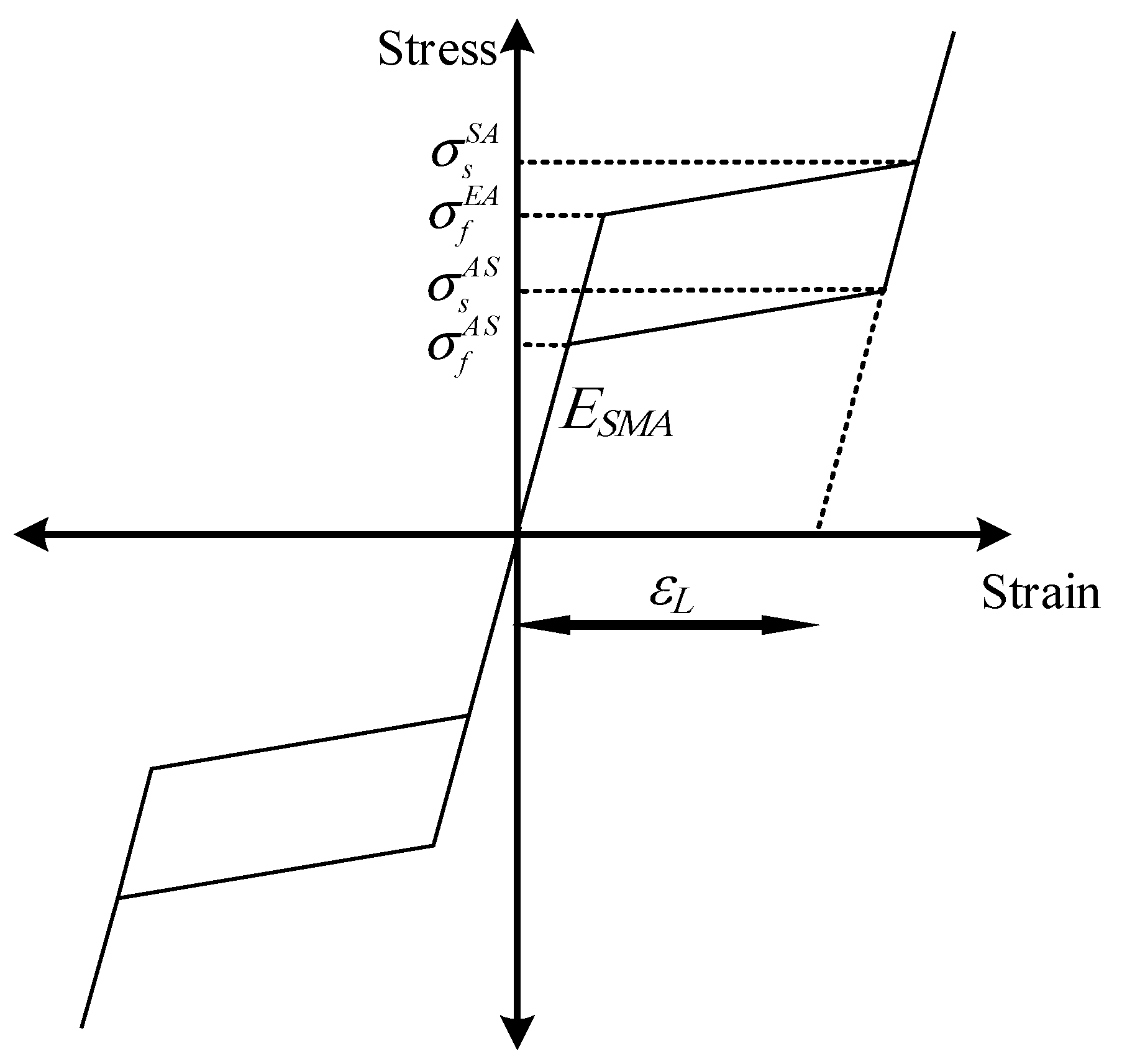
Figure 1. Shape memory and superelasticity features of SMAs [79].
Applsci 11 10057 g001
Figure 2. Stress–strain model of SMAs with superelasticity feature [81].
Applsci 11 10057 g002
Figure 3. Overall research flowchart.
Applsci 11 10057 g003
Figure 4. Schematic of ANN algorithm.
Applsci 11 10057 g004
Figure 5. Schematic of GMDH-NN algorithm.
Applsci 11 10057 g005
Figure 6. The test device of steel bar hysteretic damper and integrated isolator system.
Applsci 11 10057 g006
Figure 7. Experimental cyclic load pattern [58].
Applsci 11 10057 g007
Figure 8. Numerical model of rubber isolator equipped by SBHDs in SeismoStruct software.
Applsci 11 10057 g008
Figure 9. Hysteresis curves of experimental sample [57] and numerical model of (a) rubber isolator and (b) rubber isolator equipped with steel bar hysteretic damper.
Applsci 11 10057 g009
Figure 16. The R and MSE values at different neurons in hidden layer of ANN model: (a) β; (b) α.
Applsci 11 10057 g016
Figure 17. Measured vs. predicted β for training and testing stages using: (a) and (b) ANN (β); (c) and (d) GMDH-NN (β).
Applsci 11 10057 g017
Figure 18. Measured vs. predicted α for training and testing stages using: (a) and (b) ANN (β); (c) and (d) GMDH-NN (β).
Applsci 11 10057 g018
Figure 19. Error values in test and train stages of β in proposed models: (a,b) ANN (β); (c,d) GMDH-NN (β).
Applsci 11 10057 g019
Figure 20. Error values in test and train stages of α in proposed models: (a,b) ANN (α); (c,d) GMDH-NN (α).
Applsci 11 10057 g020
Figure 21. The effect of the input parameters on β estimation by considering R and RMSE values in proposed models: (a) ANN; (b) GMDH-NN.
Applsci 11 10057 g021
Figure 22. The effect of the input parameters on α estimation by considering R and RMSE values in proposed models: (a) ANN; (b) GMDH-NN.
Applsci 11 10057 g022
Figure 10. Schematic of SMA-BHD numerical models of variable number of bars: (a) one; (b) two; (c) three; (d) four; (e) five; (f) six; (g) seven; (h) eight; (i) nine; (j) ten.
Applsci 11 10057 g010
Figure 11. Typical hysteresis curves of SMA-BHD numerical models with 50 mm diameter (Φ50) and different number of bars in Set 1: (a) one; (b) two; (c) three; (d) four; (e) five; (f) six; (g) seven; (h) eight; (i) nine; (j) ten.
Applsci 11 10057 g011
Figure 12. Typical hysteresis curves of SMA-BHD numerical models with 10 numbers of bars of different cross-sectional diameters in Set 1: (a) Φ18; (b) Φ20; (c) Φ22; (d) Φ24; (e) Φ26; (f) Φ28; (g) Φ30; (h) Φ32; (i) Φ34; (j) Φ36; (k) Φ38; (l) Φ40; (m) Φ42; (n) Φ44; (o) Φ46; (p) Φ48 and (q) Φ50.
Applsci 11 10057 g012
Figure 13. Idealisation of hysteresis curve using bilinear envelope curve.
Applsci 11 10057 g013
Figure 14. Adopted bilinear curve for obtaining seismic parameters.
Applsci 11 10057 g014
Figure 15. The process of Q_Bi. determination.
Applsci 11 10057 g015
Table 1. Mechanical properties of SMA materials.
Mechanical PropertySet 1Set 2Set 3
ESMA (GPa)3024.628
εL (‰)4.84.104.25
σfEA (Mpa)350280320
σsSA (MPa)370350460
σsAS (MPa)150250260
σfAS (MPa)13540190
Table 2. Statistical properties of the numerical database.
Mechanical PropertyInputsOutputs
Statistical FeatureD (m)L (m)NE (GPa)Fy (MPa)β_Bi.α_Bi.
Min0.0180.324124.62800.0050.061
Max0.0501.36210303500.0400.720
Ave0.0370.7286.28627.658318.2740.0220.268
SD0.0080.2412.5972.20328.5640.0080.110
CoV (%)24.01632.90141.3038.0108.97736.72541.720
Table 3. ANNs performances for optimised β model.
NNMSE_TrMSE_TsMAPE_TrMAPE_TsR_trainR_testR_valid
30.005030.0066318.8619.800.83550.77150.8399
40.005560.0089419.4422.070.80890.79800.7799
50.002370.005189.1610.760.92830.92740.8995
60.000120.000472.603.310.99720.99580.9916
70.003390.0036211.9112.120.88400.83880.8082
80.000590.002235.327.610.98840.94610.9847
90.002040.004209.8413.160.93920.94130.9063
100.002110.0047511.3316.830.94100.85420.9528
110.002200.0042412.1217.430.94930.87660.9017
120.000710.002606.139.420.98490.97170.9470
130.000680.001865.888.750.98330.95680.9713
140.000650.002584.698.040.99300.94700.9733
150.001150.002408.1211.350.97770.91230.9537
160.000860.002767.3112.710.98750.89580.9543
170.000500.002065.6410.360.99130.96170.9756
180.004080.0051315.9618.470.84950.82220.8120
190.001240.004129.4715.320.97530.90340.9403
200.000570.001826.279.780.98530.96010.9806
210.001540.003899.4014.160.97630.84080.9180
220.001400.004248.2113.340.98410.88500.9081
230.000930.002656.0210.570.98910.90170.9717
240.001120.002938.3114.380.97130.92910.9634
250.003840.0075315.5620.610.90240.67010.8679
Table 4. ANNs performances for optimised α model.
NNMSE_TrMSE_TsMAPE_TrMAPE_TsR_trainR_testR_valid
30.004240.0048115.9215.730.88920.85400.8898
40.005160.0056919.5218.710.86090.85670.7405
50.001540.001938.598.860.96560.94440.9369
60.000200.000304.114.300.99560.99170.9936
70.002450.0027510.0510.180.93300.89410.9229
80.003040.0034710.8911.100.92090.89010.8737
90.004210.0050115.7615.510.88390.83810.8575
100.000070.000082.342.430.99860.99660.9972
110.000230.000344.314.770.99540.98900.9904
120.000110.000152.823.200.99830.99380.9920
130.000110.000142.873.140.99810.99660.9927
140.000110.000212.702.940.99830.98900.9967
150.000130.000253.023.820.99780.99150.9943
160.000070.000092.132.450.99920.99390.9952
170.000070.000112.172.610.99920.99250.9967
180.000170.000372.913.470.99750.99060.9920
190.000090.000192.453.150.99910.99500.9941
200.000140.000202.923.390.99790.98950.9941
210.000070.000122.132.750.99910.99570.9958
220.000180.000442.613.810.99910.98930.9871
230.000150.000282.994.150.99800.98920.9943
240.000210.000343.233.990.99790.98120.9896
250.000250.000483.885.150.99720.98390.9894
Table 5. The weights and bias of the β and α using ANN (β) and ANN (α).
ANN
Model
Neuron
Number
WeightBias
WikWk
D (m)L (m)NE (Pa)Fy (Pa)bhkb0
ANN (β)13.965−20.960−0.6190.187−0.62010.051−17.34710.821
2−1.1084.5410.1320.415−0.8373.7841.343
3−1.1935.3740.2161.576−1.959−1.8530.845
4−2.0518.0780.2610.024−0.998−5.0043.198
51.0080.1080.6450.208−0.0591.520−2.189
62.392−9.337−0.3151.584−0.635−3.428−3.944
ANN (α)10.559−2.633−0.2761.729−2.516−3.1411.2163.533
21.366−4.664−0.196−0.5202.946−0.5200.335
30.843−2.784−0.621−1.609−2.580−0.2522.271
4−0.6162.5990.258−0.8181.907−3.149−1.095
50.947−0.2720.5382.2542.0550.7412.634
6−0.321−2.1570.185−0.1330.139−0.250−1.712
7−0.6733.0860.070−0.913−0.159−2.3421.988
8−0.9625.9210.5610.3502.526−0.3533.006
9−1.3007.7810.3641.100−0.862−4.0837.370
100.833−3.854−0.1852.809−1.610−2.730−2.643
Table 6. The errors and performances of ANN and GMDH-NN models.
ParameterMethodData
Partition
RR2MSERMSEMAEMAPE (%)
βANN (β)Training0.99740.99490.000080.009030.005720.91
Testing0.99170.98340.000240.015380.007731.18
GMDH-NN (β)Training0.97260.94590.005540.074410.055073.55
Testing0.97440.94940.004230.065070.050803.03
αANN (α)Training0.99860.99720.000040.005970.004442.23
Testing0.99850.99710.000030.005780.004642.21
GMDH-NN (α)Training0.95970.92100.001000.031590.0233410.90
Testing0.96850.93790.000700.026420.019918.16
Publisher’s Note: MDPI stays neutral with regard to jurisdictional claims in published maps and institutional affiliations.

