Modeling the Trip Distributions of Tourists Based on Trip Chain and Entropy-Maximizing Theory

Abstract

Suburban tourist railway is an emerging transportation mode for tourism. Knowing the travel demand and trip distribution patterns of tourists is an important prerequisite to the planning and construction of suburban tourist railways. However, this issue has attracted very little research attention so far. Therefore, this paper proposes a forecasting model focused on the trip distribution of tourists who travel with the suburban tourist railway. Based on the analysis of the characteristics of tourists’ trips and the use of the trip chain method, the frequency, order, distance, and visiting volume of stay points of the trips of tourists have been intensively studied. Then, a tourist trip distribution forecasting model was built in this paper. It uses the Entropy-Maximizing theory to predict trip chain distribution probability and obtain the distribution of tourists within the city. A case study that takes the H city as an example was conducted to test the proposed model. The results of this case show that the output of the model can reflect the real trip distribution characteristics of tourists very well, which demonstrates the applicability and effectiveness of the proposed model.

1. Introduction

With the development of tourism and suburban railways, the suburban tourist railway has become an emerging solution to meet the needs of “fast move, slow tourism” [1,2] for tourists. A suburban tourist railway connects the tourist attractions, transportation hubs, and passenger distributing centers located in the urban and suburban areas of a city. It also has the characteristics of rail transit such as large capacity and comfort, and is both fast and safe [3,4]. This indicates that suburban tourist railway could significantly optimize the tourist traffic network of a city, enhancing the connections between urban and suburban tourist attractions, so as to bring great benefits (e.g., efficiency and convenience) to the tourists, the tourism industry, and the transportation systems of the city, especially when facing a large number of tourists and heavy traffic congestion. Thus, the construction of suburban tourist railways, including the feasibility analysis, planning, and design, is of great importance to a city’s tourist transport and economy. Knowing the transport demand and trip distribution patterns of tourists is an important prerequisite to the planning and construction of suburban tourist railways. Therefore, the research of tourist flow spatial distribution forecasting models is an important issue in the development of the suburban tourist railway.

In recent years, considerable efforts have been devoted to the research of tourists’ trip activities and transport demand forecasting models. In terms of the trip activity analysis, Xu et al. [5] established the gravitational order of tourist flow to tourism cities in different periods based on the analysis of the characteristics of tourist flow. Li and Lin [6] examined the spatial–temporal dynamics of tourist flow in tourist destinations and built the spatial concentration index model and the tourism center of gravity model. Song and Guo [7] analyzed the travel laws of tourists using mobile communication big data and established a statistical model based on the big data of tourist flow. On the other hand, the most commonly used trip distribution forecasting methods are aggregate and disaggregate models [8]. Aggregate models mainly include the growth-factor methods (e.g., the Fratar method), gravity models [9,10,11], and intervening opportunities models [12]. In particular, the gravity models have later been explained using the maximum entropy theory and maximum likelihood principle. The intervening opportunities model was modified by Sheffi [13] to make it more widely used. Disaggregate models include random utility models such as Logit and Nested Logit [8]. In the last few decades, activity-based models which view travel as a demand derived from travelers’ needs to participate in activities have attracted much attention [14,15]. In this context, based on the travel laws of tourists, Tian et al. [16] proposed a trip distribution model using trip chain [17,18], a sequence of linked trip segments between a pair of anchor activities, as the unit of trip distribution analysis. This makes it different from traditional trip distribution models [19] in which the trips are independent from each other. Besides, Tang et al. [20] reported a new method based on the Entropy-Maximizing (EM) theory to model the Origin–Destination (OD) distribution of taxi trips. Prior probability was used in it to improve the prediction performance of trip distribution. Furthermore, new data sources and techniques such as social media data and Machine Learning (ML), respectively, have been increasingly used to improve the predictive power and accuracy of trip distribution models [21,22]. In summary, these methods have significantly improved the understanding of tourists’ trip activities and transport demand. However, existing studies mainly focus on the model of trip distribution of traditional transportation modes; very little attention has been paid so far to solve the problem of forecasting the tourist flow distribution of a suburban tourist railway. As a result, planners and policy-makers from the local government of a tourist city still lack proper methods and solid evidence to plan and design suburban tourist railways.

To fill this gap, this paper proposes a method based on the Entropy-Maximizing theory and trip chain to model the tourist flow distribution of suburban tourist railway. By analyzing the trip distribution characteristics of tourists (Section 2), a trip chain-based model was built to describe the trip distribution of tourists (Section 3). Then, a tourist flow distribution forecasting model for the suburban tourist railway was built based on the trip chain model and Entropy-Maximizing theory (Section 4). A case study was conducted using trip distribution data collected from the tourists who take suburban tourist railways around the H city to demonstrate the use of the proposed method (Section 5). Analysis of the results shows that the model can reflect the real trip distribution characteristics of tourists very well. Section 6 provides the conclusions of this paper.

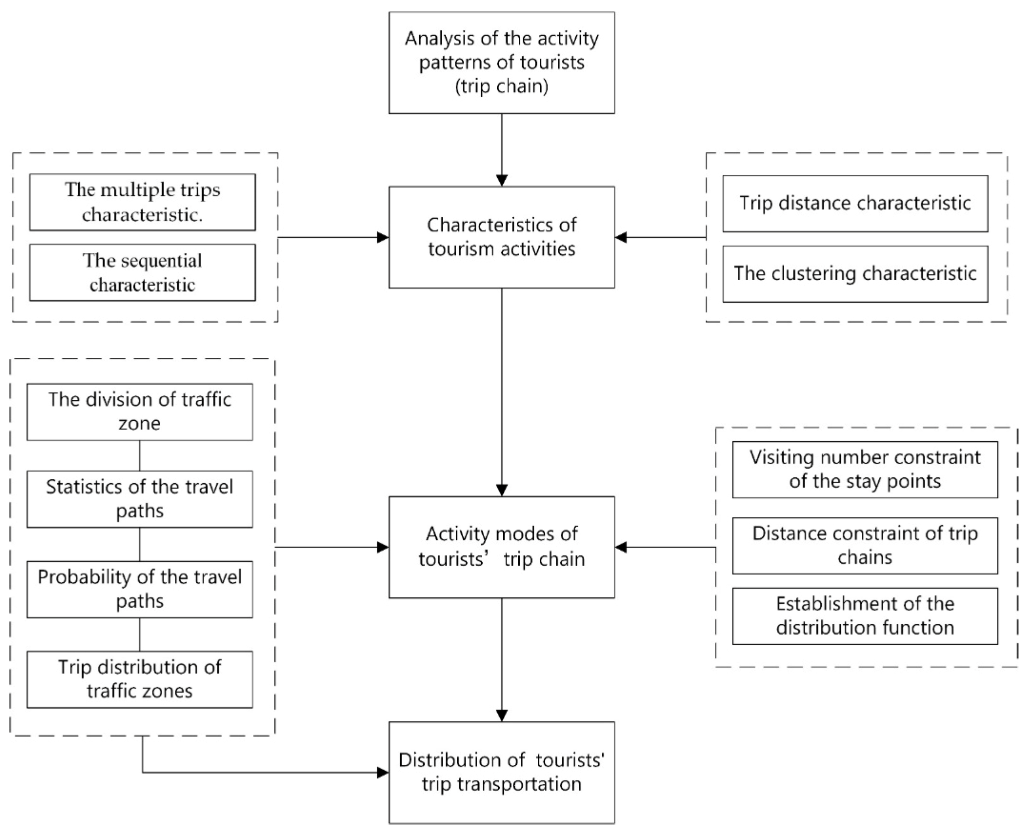
2. Trip Distribution Characteristics of Suburban Tourism Activities

Tourism activity refers to the process that tourists take time and space for tours and sightseeing. Tourism activities could be influenced by many factors such as the number, distribution, trip distance, and attraction of scenic spots. Normally, tourists attracted by multiple scenic spots will organize multiple trips and activities in a certain order. Thus, tourism activities within a city‘s suburbs could have many kinds of modes (Figure 1).

The primary characteristics of tourism activities are listed below:

• The multiple trips characteristic. Tourists usually like to visit multiple scenic spots when they travel in a tourism city. Each visit to a scenic spot is recorded as a trip. Thus, tourism activity could involve multiple trips. Note that the number of trips is generally limited due to the factors such as travel time and tourists’ willingness.
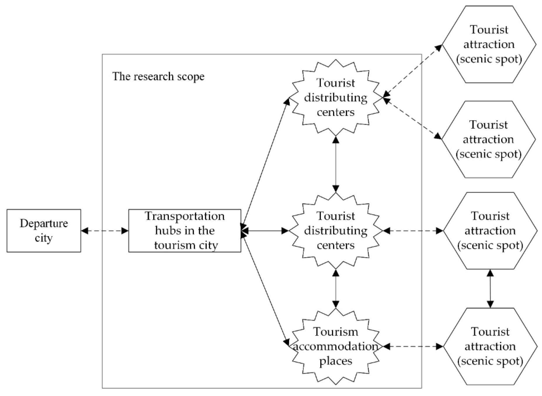
• The sequential characteristic. The travel paths of tourism activities are not randomly distributed but follow certain rules. For example, when tourists visit different scenic spots of a tourism city, they generally travel in a certain order. Specifically, they always travel starting from a departure point (e.g., a hotel or transportation hub), then arrive at various scenic spots, and finally end at an accommodation place or transportation hub. This indicates that the trips involved in tourism activity are sequential trips that can be linked as a trip chain.
• The trip distance characteristic. Activities between transportation hubs and scenic spots reflect the trip distance of tourists [23]. Trip distance between departure points and scenic spots, or between scenic spots, is a very important factor that can affect the time, costs, and experiences of tourism activities. It can be regarded as a traveling obstacle since long-distance travel is time-consuming, costly, and tiring. Thus, the scenic spots near the urban areas generally could attract more tourists.
• The clustering characteristic. Activity places of tourists in tourism cities mainly include transportation hubs, scenic spots (especially scenic spots close to each other), and accommodation places. Transportation hubs are distributing centers of tourists, scenic spots (tourist attractions) are the destinations of tourism activities, and accommodation places are the locations where tourists have rest, respectively. What they have in common is that they are the nodal areas that can attract and cluster a large number of tourists.

3. Tourist Trip Chain Modeling

3.1. Basic Idea for Trip Distribution Modeling

In traditional trip distribution models, the gravity model and growth factor model calculate trip distribution based on only one trip, whereas the tourist trip chain method takes tourists’ multiple trips into consideration, which can be viewed as chaining of trips. The trips of tourists in a trip chain have a chain structure in which tourists start from the origin point, then visit several scenic spots, and finally arrive at the destination point. The trip chain reflects the actual trips of tourists and every tourist has a trip chain. Using the trip chain method to investigate the travel activities of tourists can reveal the order, frequency, distance, and the number of tourists at the stay points of tourists’ trips. This accords with the trip distribution characteristics of tourism activities.

A study area can be divided into multiple traffic zones according to the scenic spots and transportation hubs. These traffic zones can be regarded as stay points in trip chains. Thus, the tourist trip chain becomes chaining of the activities between traffic zones. Then, to predict the spatial distribution of tourists based on the activity modes of the tourists’ trip chain, the first step is to count the number of traffic zones in the tourism city, the next is to clarify the trip chain types and count the number of types according to the statistic of traffic zones and the characteristics of tourists’ trips. Besides, each of the stay points is both the ending point of the last trip and the starting point of a new trip, which implies they would cluster a certain number of tourists. Thus, we can calculate the amount of attraction and production of tourists for each traffic zone. Then, based on the visiting number and trip distance constraints of the stay points, distribution functions could be established to calculate the probability of the type of each trip chain. After that, the trip volume of each trip chain in the traffic zone can be obtained, as well as the volume of trip distributions between each zone. Figure 2 depicts the overall process.

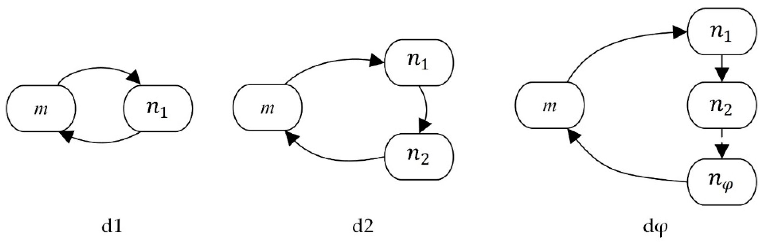
3.2. Basic Definitions of Tourist Trip Chain

A trip refers to the travel of people, goods, or cars as a means of transportation from one place to another [24]. Specifically, the travel of people is called personal or individual trips. Meanwhile, a trip chain is defined as a round trip consisting of people completing one or more activities in chronological order and contains a large amount of information about the time, space, ways, and activities of the trip [25]. The structure of a trip chain generally consists of multiple segments, each of which is recorded as a trip. Thus, a tourist trip chain is a set of sequential trips taken by tourists who participate in one or more tourism activities for tours and sightseeing [26]. Normally, we define the departure point of the trip chain as the starting point, the final destination of the trip chain as the ending point, and the points in the middle of the trip chain as stay points.

To facilitate the study, this paper divides tourist destinations into different traffic zones. These traffic zones can be further classified into several types, including scenic spot-dominated traffic zones, transportation hub-dominated traffic zones, city entrance/exit-dominated traffic zones, and traffic zones in other areas of the city. These traffic zones have corresponding relationships to the starting point, ending point, and stay points of a trip chain. Generally, the starting point and ending point of the trip chain are the traffic zones dominated by the transportation hub or the entrance/exit of the city, respectively; the stay points are the scenic spot-dominated traffic zones or the traffic zones in other areas of the city. Meanwhile, each traffic zone can either be the starting point or ending point of a trip within a trip chain. To keep things simple, this paper defines the starting point of a trip as the origin zone, and the ending point of a trip as the destination zone.

Trip chains can be further divided into simple and complex chains according to their complexity. A simple trip chain consists of two consecutive trips and has only one stay point. A complex trip chain consists of more than two consecutive trips and has more than one stay point.

To analyze the trip types of each tourist, this paper uses $m$ to represent the origin zone and $m=\left\{1, 2, 3,\dots ,M \right\}$, M is the maximum number of origin zones. Similarly, we use $n$ to represent the destination zone and $n=\left\{1, 2, 3,\dots ,M \right\}$, N is the maximum number of destination zones. Then, as shown in Figure 3, the trip of a tourist that starts from origin zone $m$ to a number of destination zones $\left\{n_1,n_2,n_3,\dots ,n_{\phi } \right\}$ and finally returns to $m$ again has a chain structure. Here, φ is the maximum number of destination zones that a tourist could visit in a trip chain. Then, we can define the choice set for trips starting from an origin zone as $H=\left\{d_1,d_2,d_3\dots ,d_{\phi }\right\}$. It is a set of trip chains that have selected φ numbers of destination zones and is called the φ dimensional destination zone choice set hereafter.

3.3. The Number of Tourist Trip Chains

To facilitate the analysis of tourists‘ trip chains, this paper specifies that the origin and destination zones in a trip chain are not the same. Furthermore, each trip in a trip chain starts from one traffic zone to another, and there are no repeated traffic zones in a trip chain. This means there are no cyclic structures within the trip chain formed by traffic zones.

Therefore, it can be defined that the length of a trip chain is the number of selected destination zones in that chain. Consequently, the maximum length of the trip chains of a choice set is the maximum number of destination zones that can be selected, i.e., the value of $\phi$. Then, suppose a trip distribution model has a φ dimensional destination zone choice set, because the number of trip chains in a choice set should be less than or equal to the maximum number of accessible destination zones (J), i.e., $1\le \phi \le J$, so the number of trip chains in the model is equal to $M\times \left(A_J^1+A_J^2+\dots +A_J^{\phi }\right)$, where M is the maximum number of the origin zones, and the calculation of $A_J^{\phi }$is based on the permutation formula. For example, if a tourist intent to visit three scenic spots, both the number of origin zones and destination zones is three, and the maximum length of the trip chain is three (i.e., $\phi =3$), then the dimension of the traffic zone choice set is no more than three, and the number of trip chains is $3\times \left(A_3^1+A_3^2+A_3^3\right)=45$.

In practice, the length of a trip chain and further the number of trip chains can be calculated according to the travel behavior of tourists. More specifically, it can be estimated through a questionnaire survey of tourists about the time and distance required to finish the trips.

4. The Trip Distribution Forecasting Model Based on Trip Chains

Based on the trip chain method proposed to analyze the distribution of tourists, this section uses the Entropy-Maximizing theory to model the probability of tourists’ trip distribution. Two types of trip chain constraints, i.e., the visiting volume constraint of stay points and the travel distance constraint, were defined based on the characteristics of trip chains. Then, a trip chain-based trip distribution model was built, along with the corresponding model-solving algorithm.

4.1. Trip Chain Constraints

4.1.1. Visiting Volume Constraint of Stay Points

The trip volume of a trip chain is normally distributed in the involved traffic zones. This means its value is constrained by the amount of produced and attracted trips in the origin and destination zones. By dividing scenic spots and transportation hubs into many traffic zones, the amount of tourist production and attraction in each traffic zone could be easily inferred based on the collected number of tourists in scenic spots and the traffic volume of transportation hubs. This enables us to define restrictive conditions (i.e., constraints) on the amount of tourist production and attraction of origin and destination zones of a trip chain. Suppose every tourist departure from the traffic zone m, and the selected trips choice set is H, then the visiting volume constraint of stay points of a trip chain can be defined as Equation (1):

$$\{\begin{array}{c}{O}_m={\displaystyle \sum _{H\in H^a}}{S}_{mH}, m=\left\{1,2,\dots ,M\right\}\hfill \\ D_n={\displaystyle \sum _{j=1}^J}{\displaystyle \sum _{m=1}^M}{\displaystyle \sum _{(H\in H^a|n=n_j)}}{S}_{mH}, n=\left\{1,2,\dots ,N\right\}\hfill \end{array}$$

(1)

where O_m means the produced trip volume of origin zone m; D_n is the number of tourists that arrive at destination zone n;$H^a$ is the destination zone choice set of tourists, and $S_{mH}$ denotes the volume of trips that select H as the choice set for trip chains which start from origin zone m. Since every trip chain starts from an origin zone, so the number of tourists of origin zone m (i.e., O_m) is the sum of trip volumes of all the trip chains that start from origin zone m. Similarly, the number of tourists of destination zone n (i.e., D_n) is the sum of tourists of the trip chains that start from the origin zone m and take the traffic zone n as the jth destination zone, i.e., the number of tourists whose trip chains start from origin zone m and pass through the traffic zone n.

4.1.2. Trip Distance Constraint

The actual trip distance of tourists in a tourism city with a complex traffic network reflects the distance limitation of tourist trip chains. Generally, when calculating trip impedance, the trip distance or time should be calculated according to the actual traffic network. Thus, to obtain the actual trip distance between traffic zones and further calculate trip impedance, it is necessary to establish a tourism traffic network, and take into consideration the length and interaction of public transit roads, railways, and other types of transit adopted by tourists to travel. The needs for data preparation and processing should also be considered.

The trip distance of a tourist’s travel from an origin traffic zone to a destination traffic zone is normally limited within a certain range of tourist destinations. Thus, the constraint of the total trip distance of tourists can be defined as Equation (2):

$$d=\sum _{m=1}^M\sum _{H\in H^a}{S}_{mH}\times d_{mH}$$

(2)

where d represents the total trip distance, and $d_{mH}$ is the trip distance of different choice sets in which the trip chains take m as the origin traffic zone.

4.2. Trip Distribution Forecasting Model

4.2.1. Objective Function

Let $P\left(S_{mH}\right)$ be the probability of a tourist trip chain, then we can establish the objective function of the tourist trip chain probability distribution as Equation (3):

$$P\left(S_{mH}\right)=\frac{S!}{{\prod }_{m=1}^M{\prod }_{H\in H^a}{S}_{mH}!}\prod _{m=1}^M\prod _{H\in H^{\alpha }}{\left(P_{mH}\right)}^{S_{mH}}$$

(3)

where S is the total number of trip volumes.

4.2.2. Model Building

This paper uses the Entropy-Maximizing theory to build a trip distribution model. According to the Entropy-Maximizing theory, the maximum value of $P(S_{mH})$ is trip chain probability distribution. Specifically, when entropy reaches its maximum value, the $P\left(S_{mH}\right)$ of a trip chain reaches the maximum. Therefore, the trip distribution forecasting model can be transformed into an optimal objective programming problem, as shown in Equation (4):

$$\begin{array}{c}\max P\left(S_{mH}\right)=\frac{S!}{{\prod }_{m=1}^M{\prod }_{H\in H^a}{S}_{mH}!}{\displaystyle \prod _{m=1}^M}{\displaystyle \prod _{H\in H^{\alpha }}}{\left(P_{mH}\right)}^{S_{mH}}\hfill \\ st.\{\begin{array}{c}{O}_m={\displaystyle \sum _{H\in H^a}}{S}_{mH}, m=\left\{1,2,\dots ,M\right\}\hfill \\ D_n={\displaystyle \sum _{j=1}^J}{\displaystyle \sum _{m=1}^M}{\displaystyle \sum _{H\in H^a|n=n_j}}{S}_{mH}, n=\left\{1,2,\dots ,N\right\}\hfill \\ d={\displaystyle \sum _{m=1}^M}{\displaystyle \sum _{H\in H^a}}{S}_{mH}\times d_{mH} \hfill \end{array}\hfill \end{array}$$

(4)

Then, we take logarithms of the objective function and use the Stirling approximation formula, i.e., $\ln x!=x\ln x-x$, to transform the objective function into Equation (5):

$$\begin{array}{c}lnP\left(S_{mH}\right)=\ln S!-{\displaystyle \sum _{m=1}^M}{\displaystyle \sum _{H\in H^a}}{S}_{mH}+{\displaystyle \sum _{m=1}^M}{\displaystyle \sum _{H\in H^a}}{S}_{mH}\ln P_{mH}\hfill \\ =\ln S!-{\displaystyle \sum _{m=1}^M}{\displaystyle \sum _{H\in H^a|m=j}}\left(S_{mH}ln{S}_{mH}-S_{mH}\right)+{\displaystyle \sum _{m=1}^M}{\displaystyle \sum _{H\in H^a|n=n_j}}{S}_{mH}ln{P}_{mH}\hfill \end{array}$$

(5)

Focusing on the abovementioned optimization problem, we build the Lagrangian formula and insert the constraint conditions into it. The result is shown in Equation (6).

$$\begin{array}{c}L\left(S_{mH},\alpha ,\beta ,\gamma \right)=\ln S!-{\displaystyle \sum _{m=1}^M}{\displaystyle \sum _{H\in H^a}}(S_{mH}ln{S}_{mH}-S_{mH})\hfill \\ +{\displaystyle \sum _{m=1}^M}{\displaystyle \sum _{H\in H^a}}{S}_{mH}ln{P}_{mH}+{\displaystyle \sum }_{m=1}^M{\alpha }_m\left(O_m-{\displaystyle \sum _{H\in H^a}}{S}_{mH}\right)\hfill \\ +{\displaystyle \sum }_{n=1}^N{\beta }_n\left(D_n-{\displaystyle \sum }_{j=1}^J{\displaystyle \sum }_{m=1}^M{\displaystyle \sum _{H\in H^a|n=n_j}}{S}_{mH}\right)\hfill \\ +\gamma \left(d-{\displaystyle \sum }_{m=1}^M{\displaystyle \sum _{H\in H^a}}{S}_{mH}{d}_{mH}\right)\hfill \end{array}$$

(6)

where α, β, and γ are Lagrangian operators.

Further, we take partial derivatives of $S_{mH}$, α, β, and γ, respectively, and set them to zero, then we get Equation (7):

$$\{\begin{array}{c}\frac{\partial L}{\partial S_{mH}}=-\ln S_{mH}+\ln P_{mH}-{\alpha }_m-\phi {\beta }_n-\gamma d_{mH}=0 \hfill \\ \frac{\partial L}{\partial \alpha }=O_m-{\displaystyle \sum _{H\in H^a}}{S}_{mH}=0\hfill \\ \frac{\partial L}{\partial \beta }={\displaystyle \sum _{j=1}^J}{\displaystyle \sum _{m=1}^M}{\displaystyle \sum _{H\in H^a|n=n_j}}{S}_{mH}=0\hfill \\ \frac{\partial L}{\partial \gamma }=d-{\displaystyle \sum }_{m=1}^M{\displaystyle \sum _{H\in H^a}}{S}_{mH}{d}_{mH}=0\hfill \end{array}$$

(7)

where φ is the length of a trip chain. Thus, the result of $S_{mH}$ is:

$$S_{mH}=P_{mH}\exp \left(-{\alpha }_m-\phi {\beta }_n-\gamma d_{mH}\right)$$

(8)

Besides, the constraints of the amount of trip production and attraction can be represented as Equation (9):

$$\{\begin{array}{c}{O}_m=\mathrm{e}\mathrm{x}\mathrm{p}\left(-{\alpha }_m\right){\displaystyle \sum _{H\in H^a}}{P}_{mH}\exp \left(-\phi {\beta }_n-\gamma d_{mH}\right)\hfill \\ D_n=\mathrm{e}\mathrm{x}\mathrm{p}\left(-{\beta }_n\right){\displaystyle \sum _{j=1}^J}{\displaystyle \sum _{m=1}^M}{\displaystyle \sum _{H\in H^a|n=n_j}}{P}_{mH}\exp \left[-{\alpha }_m-\left(\phi -1\right){\beta }_n-\gamma d_{mH}\right]\hfill \end{array}$$

(9)

To simplify the representation of the model, we define that:

$$\{\begin{array}{c}{R}_m=\frac{\exp \left(-{\alpha }_m\right)}{O_m}\hfill \\ T_n=\frac{\exp \left(-{\beta }_n\right)}{D_n}\hfill \end{array}$$

(10)

Thus, $S_{mH}$ can be represented as Equation (11):

$$S_{mH}=R_m{O}_m\left({\displaystyle \prod _{n=1}^{\phi }}{T}_n{D}_n\right)P_{mH}exp\left(-\gamma d_{mH}\right)$$

(11)

Then, parameter $R_m$ and $T_n$ can be represented as Equation (12):

$$\{\begin{array}{c}{R}_m={\left[{\displaystyle \sum _{H\in H^a}}\left({\displaystyle \prod _{n=1}^{\phi }}{T}_n^{\lambda }{D}_n\right)P_{mH}\exp \left(-\gamma d_{mH}\right)\right]}^{-1}\hfill \\ T_n={\left[{\displaystyle \sum _{j=1}^J}{\displaystyle \sum _{m=1}^M}{\displaystyle \sum _{H\in H^a|n=n_j}}{R}_m{O}_m({\displaystyle \prod _{\begin{array}{c}{n}^{*}=1\\ n^{*}\ne n\end{array}}^{\phi }}{T}_{n^{*}}{D}_{n^{*}})P_{mH}\exp \left(-\gamma d_{mH}\right)\right]}^{-1}\end{array}$$

(12)

where λ is the number of iterations. Put Equation (11) into the trip chain distance constraint (i.e., Equation (2)), we can represent the trip distribution forecasting model as Equation (13):

$$f\left(\gamma \right)={\displaystyle \sum _{m=1}^M}{\displaystyle \sum _{H\in H^a}}{R}_m{O}_m\left({\displaystyle \prod _{n=1}^{\phi }}{T}_n{D}_n\right)P_{mH}\exp \left(-\gamma d_{mH}\right)d_{mH}-d=0$$

(13)

4.2.3. Model Solving

This section provides the solution to calculate the value of α, β, and γ of Equation (8), and further calculate the parameter γ, $R_m^{\lambda +1}$, and $T_n^{\lambda +1}$ (see Equation (14) below) according to Equation (10). In this solution, the number of produced trips of origin zone m (i.e., $O_m$) and the number of trip chains of destination zone n within the tourism cities of the study area, as well as the total trip distance (i.e., d) obtained according to the traffic network of the tourism city, are already given. The proposed model solving steps of this solution are described in Figure 4.

Detailed steps and explanations of this solution are listed as follows:

• step 1: initialize parameter values, let γ = 1, λ = 1, $T_n^0=1$, and the value of random residual ε = 0.05;
• step 2: calculate $R_m^{\lambda +1}$ and $T_n^{\lambda +1}$ according to Equation (14):

  $$\{\begin{array}{c}{R}_m^{\lambda +1}={\left[{\displaystyle \sum _{H\in H^a}}\left({\displaystyle \prod _{n=1}^{\phi }}{T}_n^{\lambda +1}{D}_n\right)P_{mH}\exp \left(-\gamma d_{mH}\right)\right]}^{-1}\hfill \\ T_n^{\lambda +1}={\left[{\displaystyle \sum _{j=1}^J}{\displaystyle \sum _{m=1}^M}{\displaystyle \sum _{H\in H^a|n=n_j}}{R}_m^{\lambda +1}{O}_m({\displaystyle \prod _{\begin{array}{c}{n}^{*}=1\\ n^{*}\ne n\end{array}}^{\phi }}{T}_{n^{*}}{D}_{n^{*}})P_{mH}\exp \left(-\gamma d_{mH}\right)\right]}^{-1}\hfill \end{array}$$

  (14)

  where $m=\left\{1, 2, 3,\dots ,M\right\}$, $n=\left\{1, 2, 3,\dots ,N\right\}$.
• step 3: judge the two conditions $\left|R_m^{\lambda +1}-R_m^{\lambda }\right|/R_m^{\lambda +1}<\epsilon$ and $\left|T_n^{\lambda +1}-T_n^{\lambda }\right|/T_n^{\lambda }<\epsilon$ iteratively, if they satisfy, then go to step 4, otherwise let $\lambda +1$ and back to step 2;
• step 4: let $x^k={\gamma }^k$ and calculate ${\gamma }^k$ iteratively using Newton’s method, as shown in Equation (15):

  $$\{\begin{array}{c}{x}^{k+1}=x^k-\frac{f\left(x^k\right)}{f^{\prime }\left(x^k\right)}\hfill \\ f\left(x\right)={\displaystyle \sum _{m=1}^M}{\displaystyle \sum _{H\in H^a}}{R}_m{O}_m({\displaystyle \prod _{n=1}^{\phi }}{T}_n{D}_n)P_{mH}\exp \left(-\gamma d_{mH}\right)d_{mH}-d\hfill \\ f^{\prime }\left(x\right)=-{\displaystyle \sum _{m=1}^M}{\displaystyle \sum _{H\in H^a}}{R}_m{O}_m({\displaystyle \prod _{n=1}^{\phi }}{T}_n{D}_n)P_{mH}\exp \left(-\gamma d_{mH}\right)d_{mH}^2\hfill \end{array}$$

  (15)

  if the iterative calculation satisfies the condition $\left|x^{k+1}-x^k\right|/x^k<\epsilon$, then end the iteration, otherwise let ${\gamma }^{k+1}=x^{k+1}$.
• step 5: let $\lambda =\lambda +1$, then go back to step 2.

4.2.4. Model Inputs, Outputs, and Application

Application of the Entropy-Maximizing -based trip chain distribution model requires several types of input data, including the tourist survey data, traffic network, and traffic zones of the tourism city, as well as the number of produced and attracted tourists of each traffic zone obtained through the questionnaire survey of tourists. The prior probability of each trip chain is needed too. Then, we can get the actual probability of each trip chain and the trip distributions of traffic zones.

• Model inputs.

The input of the model includes the number of produced and attracted tourists of each traffic zone, the prior probability of trip chains, and the total trip distance between each traffic zone.

The numbers of tourists in each traffic zone are a precondition of the model. Thus, the number of origin and destination zones should be determined before preparing model input data. The origin zone is the area primarily influenced by transportation hubs, and the destination zone is the area dominated by a scenic spot. Tourist productions or attractions of these traffic zones are important input data of the model.

The prior probability of the initial travel path can be obtained from the survey data. Trip distance is not only a model constraint but also an important input of the model. It can be divided into different classes according to the types of tourists’ trips by means of aggregation. Then, the trip distance of each trip chain can be calculated separately, and the trip type of each trip distance class is taken as the input parameter of the model.

2.

Model outputs.

The output of the model is the trip probability of each trip chain. Then, we can perform a statistic analysis on the number of trips and verify whether the classification of the number of trips is consistent with the actual trips of tourists. Furthermore, trip distances can also be obtained from the model, and the distribution of the trip distances of tourists analyzed. Finally, the spatial distribution of tourists’ trips can be obtained from the model as well.

3.

Model application.

The proposed model can be used to predict the number of tourists in traffic zones in the targeted year based on the current status of the traffic zones in recent years. Specifically, according to the annual growth of tourists, the gray prediction theory can be used to predict the number of tourists in the traffic zone. Then, taking the number of tourists in the traffic zone as the input value, the model can be used to predict the trip distribution.

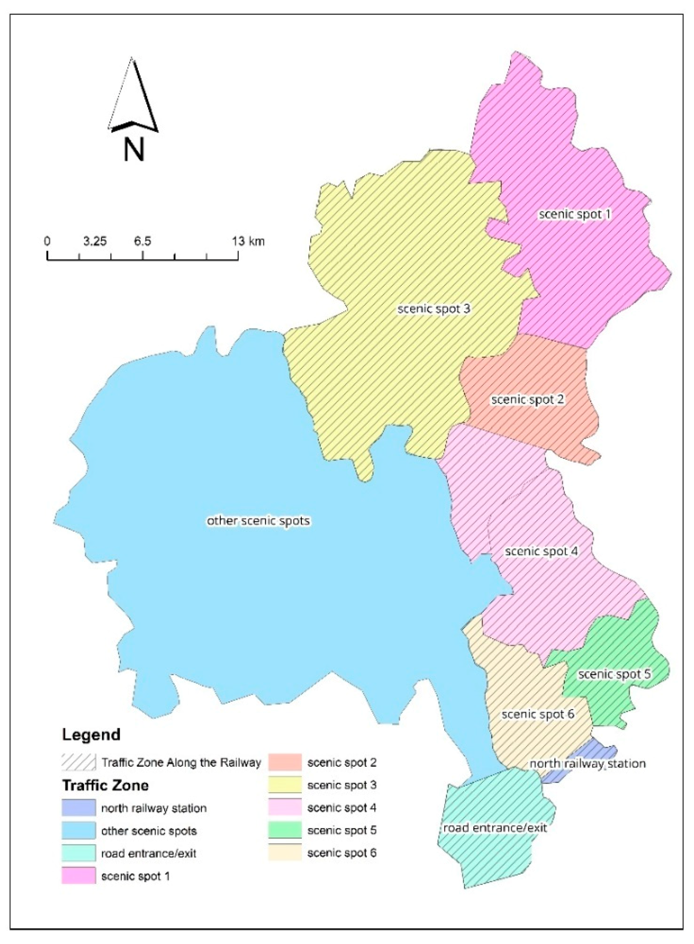
5. Case Study

5.1. Problem Statement

The suburban tourist railway Line T1 in H city is a newly built railway serving tourist passenger flow. Thus, this paper takes the region along the railway as the study area of this paper to analyze and predict the distribution of tourists’ trips. Along the railway, there are six scenic spots coded as one, two, three, four, five, and six, respectively (Figure 5). These scenic spots are divided into six traffic zones according to the location of railway stations. Besides, a virtual traffic zone is added considering the influence of tourists from other scenic spots in H city on the scenic spots along with Line T1. Additionally, two more traffic zones based on the north railway station and the entrance/exit of roads, respectively, are added in consideration of the sources of tourists. The spatial distribution of these traffic zones is shown in Figure 5.

5.2. Study Data

1.

Distributing volume of traffic zone

As mentioned above in Section 5.1, the study area was divided into nine traffic zones. The distributing volume of each traffic zone was calculated based on the tourism and traffic survey data of H city in 2019. Specifically, the tourist volume of scenic spot-dominated traffic zones was calculated according to the number of visitors of that scenic spot; the tourist volume of transportation hub-dominated traffic zones was calculated based on the number of passengers arrival and departure that transportation hub, and the tourist volume of road entrance/exit dominated traffic zones was calculated according to the volume of passenger flow obtained from the traffic survey data. The obtained tourist volume of each traffic zone is shown in

Table 1. Distributing volume of each traffic zone.

Traffic Zone Code	Traffic Zone	Trips Volume (10,000 Person/Year)
1	scenic spot 1	56
2	scenic spot 2	125
3	scenic spot 3	338
4	scenic spot 4	86
5	scenic spot 5	107
6	scenic spot 6	42
7	other scenic spots	400
8	north railway station	379
9	traffic zones based on the entrance/exit of roads	595

.

Taking traffic zones dominated by the north railway station and road entrances/exits as origin zones (i.e., traffic zones 8 and 9 in Table 1), and all the traffic zones dominated by scenic spots as destination zones (traffic zone 1~7 in Table 1), we can found that the trip attraction of the destination zones is D = {56,338,125,86,107,42,400}, the trip production of the origin zones is O = {379, 595}, and the total number of tourists is 974 (with the unit 10,000 person per year).

2.

Trip distance

Trip distance represents not only the actual distance between traffic zones but also the trip impedance such as the interaction of road and railway traffic. This section calculates the distances between traffic zones according to the trip distance constraint of the proposed model mentioned in Section 4.1.2. Firstly, traffic network data of the study area were prepared. Then, taking the centroid point of each traffic zone as the origin and destination point, the trip distance between each traffic zone was calculated using the shortest path method. The results are listed in

Table 2. Trip distances between different traffic zones (unit: m).

Traffic Zone Code	1	2	3	4	5	6	7	8	9
1	0	6586	14,709	24,801	32,110	37,291	29,416	40,013	44,567
2	6586	0	8221	18,547	26,144	31,285	23,114	34,172	38,304
3	14,709	8221	0	10,468	18,312	23,362	16,758	26,405	30,145
4	24,801	18,547	10,468	0	8025	12,936	14,990	16,090	19,774
5	32,110	26,144	18,312	8025	0	5186	19,863	8097	13,027
6	37,291	31,285	23,362	12,936	5186	0	22,423	3475	8224
7	29,416	23,114	16,758	14,990	19,863	22,423	0	25,832	24,850
8	40,013	34,172	26,405	16,090	8097	3475	25,832	0	7797
9	44,567	38,304	30,145	19,774	13,027	8224	24,850	7797	0

.

5.3. Calculation of Model Parameters

According to the survey of tourists’ trips, this study sets the average number of scenic spots visited by tourists per day no more than two. Then, let ε = 0.05; model parameters γ, $R_m$, and $T_n$ for this case can be calculated based on Equation (10). Following the steps depicted in Figure 4, after 10 iterations, it can be found that the residual is less than 0.05, and the output γ = −1.7. Figure 6 shows the relation between ε and the number of iterations. Then, based on Equation (10) and the value of $R_m$ and $T_n$, the values of parameter α and β can be calculated. Because there are two destination zones and seven origin zones, the result values of parameters α and β are ${\alpha }_1$= 10.70, ${\alpha }_2$= 10.81, ${\beta }_1$= −11.23, ${\beta }_2$= −8.84, ${\beta }_3$= −6.14, ${\beta }_4$= −5.92, ${\beta }_5$= −5.75, ${\beta }_6$= −7.24, ${\beta }_7$= −5.51.

5.4. Results and Analysis

1.

Trip chain probability distribution

Sorting the trip chains obtained by the model in descending order of the calculated probability, we obtained the first 15 trip chains as presented in

Table 3. Trip chain code and the corresponding actual trip chain.

Trip Chain Code	Actual Trip Chain	Trip Chain Code	Actual Trip Chain
93	RE1→SS2 3→RE	95	RE→SS 5→RE
87	NRS3→OSS4→NRS	875	NRS→OSS→SS 5→NRS
97	RE→OSS→RE	925	RE→SS 2→SS 5→RE
83	NRS→SS 3→ NRS	935	RE→SS 3→SS 5→RE
92	RE→SS 2→RE	91	RE→SS 1→RE
94	RE→SS 4→RE	975	RE→OSS→SS 5→RE
82	NRS→SS 2→NRS	937	RE→SS 3→OSS→RE
84	NRS→SS 4→NRS	……	……

Note: RE¹ means the road entrance/exit; SS² represents the scenic spot; NRS³ is the north railway station; OSS⁴ denotes the other scenic spots.

. The trip chain code in Table 3 represents the correspondence actual trip chain. For example, trip chain code 93 means the trip chain that starts from traffic zone 9 (see Table 1) to traffic zone 3, and then goes back to traffic zone 9.

As shown in Table 3, among the first 15 trip chains that have the maximum probability, the number of trip chains that consist of only one scenic spot is larger than the number of trip chains that involve more than two scenic spots. Specifically, the trip chain with code 93 has the maximum probability. This means tourists have the maximum probability to travel from the road entrance/exit-dominated traffic zone to scenic spot 3, and the number of tourists is also the largest. Moreover, tourists have a larger probability to travel to only one traffic zone. In particular, tourists are more likely to travel to scenic spot 3, other scenic spots, scenic spot 2, scenic spot 4, and scenic spot 5. The detailed distribution of the trip probability of trip chains listed in Table 3 is shown in Figure 7.

2.

Analysis of the trip chain types

As described in Section 3.2, this paper classifies trip chains into two types, i.e., simple trip chains and complex trip chains. Here, trip chains were classified according to the value of φ. Specifically, a trip chain with φ = 1 is a simple trip chain and φ = 2 is a complex trip chain. The proportion of simple and complex trip chains can be calculated according to the model. The trip volume of different trip chain types is shown in

Table 4. The trip volume of different trip chain types.

Trip Chain Type	Trip Probability	Trip Chain Volume	Trip Volume (Including Trip Times)
simple trip chain	0.78	7,580,051	15,120,493
complex trip chain	0.22	2,159,949	4,319,897
total	1	9,740,000	19,440,390

.

The results presented in Table 4 show that the proportion of tourism activities for simple trip chains is larger than complex trip chains. According to the maximum entropy-based trip distribution model, the maximum proportion of simple trip chains is 77.82%, and the trip volume is 15,120,493. The proportion of complex trip chains is 22.18%, and the trip volume is 4,319,897. The main reason for this might be that, when tourists visit tourism cities, a simple trip chain has a comparatively longer trip distance. This will be further discussed in the next section.

3.

Analysis of trip distance

Each trip chain has a certain distance. Thus, we can classify trip chains according to their distance. By counting the number of trip chains at an interval of 5 km, we can obtain the distribution of trip distances and the corresponding trip probability, as listed in

Table 5. Trip distance probability distribution.

Trip Distance (km)	Trip Probability
0–5	0.00
5–10	0.01
10–15	0.02
15–20	0.06
20–25	0.15
25–30	0.25
30–35	0.22
35–40	0.06
40–45	0.07
45–50	0.06
50–55	0.03
55–60	0.02
60–65	0.01
65–70	0.01
70–75	0.01
75–80	0.01
80–85	0.01

.

As illustrated in Table 5, a trip distance within the range of 25–35 km has the maximum proportion; the corresponding activity locations are traffic zones 3 and 7, namely scenic spot 3 and the other scenic spots. These two traffic zones and related trip chains also have the largest number of tourists according to Figure 7. Furthermore, the distances from the origin zones 8 and 9 to the destination zones 3 and 7 are about 30 km. Thus, it is reasonable that the model results are concentrated in the range of 25–40 km. The detailed distribution of the trip distance probability is shown in Figure 8.

4.

Analysis of trip distribution

The trip distribution calculated using the trip chain-based trip distribution model is listed in

Table 6. Trip distribution of each traffic zone (number of tourists).

	1	2	3	4	5	6	7	8	9
1	0	86	5035	34,829	142,783	77,663	115,083	59,784	139,798
2	30	0	6489	46,715	201,113	108,646	153,099	243,055	531,318
3	453	1655	0	44,640	200,411	106,623	196,085	973,308	1,981,777
4	539	2050	7680	0	7465	3878	31,080	287,882	545,574
5	658	2630	10,273	2224	0	366	25,087	373,347	668,736
6	160	633	2437	515	163	0	3896	147,907	267,426
7	5875	22,181	111,360	102,591	277,942	96,829	0	1,705,019	1,815,069
8	166,177	388,441	1,083,681	212,398	70,919	8334	1,860,353	0	0
9	401,168	872,790	2,277,997	442,236	182,525	20,797	1,752,184	0	0

.

It can be seen from Table 6 that traffic zone 8 and traffic zone 9 have a relatively large volume of trips. Thus, it can be inferred that the majority of the trips of tourists to scenic spots are based on railway and road. Note that the volume of trips between some scenic spots is very small, e.g., the trips between traffic zone 1 and 2. The main reason could be that the origin zones of these trip chains are traffic zone 8 and 9, they are far away from traffic zone 1 and 2, resulting in a small result of the model.

We can draw trip expectation lines (i.e., origin–destination flows of expected trips) based on the trip distribution, as shown in Figure 9. It shows that the volume of trips from the traffic zones based on scenic spot 3 and other scenic spots to the traffic zones based on the north railway station and the road entrances/exits is relatively large, followed by the traffic volume from the traffic zones based on scenic spot 2, 4, and 5 to the traffic zones based on the north railway station and the road entrances/exits. Constrained by the visiting volume of stay points, the trip volume of traffic zones based on transportation hubs is the largest, followed by the trip volume between traffic zones where tourists visit more. These results are consistent with the trip distribution between traffic zones.

5.

Screenline Test

To test the accuracy of trip distribution between scenic spots, the traffic volume that is already known needs to be used to make judgments. This paper sets screenlines between traffic zones to facilitate the test.

Table 7. Areas separated by screenlines.

Screenline Number	One Side of the Screenline	Another Side of the Screenline	Road Name	Line Segment
1	scenic spot 1	non-scenic spot 1	G3	scenic spot 3 and 1
			G205	scenic spot 3 and 1
2	scenic spot 3	non-scenic spot 3	Gangcun Road	scenic spot 3 and other scenic spots
			S103	scenic spot 3 and other scenic spots
			G3	scenic spot 3 and 2
3	scenic spot 2 and 4	non-scenic spot 3 and 4	G3	scenic spot 3 and 2
			S103	other scenic spots and scenic spot 4
			G205	scenic spot 4 and 5
4	scenic spot 5 and 6	non-scenic spot 5 and 6	G3	scenic spot 6 and road entrance/exit
			Yingbin Boulevard	other scenic spots and scenic spot 4
			G205	scenic spot 4 to scenic spot 5

shows the areas separated by screenlines.

Specifically, as shown in Figure 10, the boundary of the traffic zone of scenic spot 1 was set as screenline 1; the boundary of the traffic zone of scenic spot 3 was set as screenline 2; the boundary line that encloses traffic zone 2 and 4 was set as screenline 3; the boundary line that encloses the traffic zones of scenic spot 5 and 6 was set as screenline 4. Then, the road traffic volume was converted into the trip volume of tourists, and the trip OD volume was allocated to the traffic network of the screenlines.

The actual passenger flow of each screenline was obtained by calculating the annual traffic flow volume of relevant roads crossing the screenlines. It has been further converted into the number of tourists. Particularly, the traffic flow data was collected from the investigation of the number, license plate, and model of vehicles passing the road check points. Moreover, the tourist flow is distinguished from the total flow by taking buses and non-local cars as tourist traffic flow. Then, the trip distribution results obtained from the model were used to simulate the passenger flow volume at the cross-sections of screenlines. The simulated results were later used to compare with the actual trip volumes, to test the reliability of the output results of the proposed model. As shown in

Table 8. Error analysis of screenlines.

Screenline	Actual Survey Data of Tourists	Screenline Allocated Data of Tourists	Error
1	500,202	575,060	13.02%
2	3,925,237	3,504,952	−11.99%
3	2,009,114	2,176,614	7.70%
4	1,336,327	1,506,457	11.29%

, the error between the simulated passenger flow on the cross-sections of screenlines and the actual passenger flow is within 15%, which is within the acceptable error range. This indicates that the model has certain reliability and can be applied to predict the trip distribution of tourists of the suburban tourist railway in the future.

6. Conclusions

Aiming to predict the trip distribution of tourists of the suburban tourist railway, this paper proposed a forecasting model based on the Entropy-Maximizing theory and the trip chain method. A case study was conducted in this paper to demonstrate the applicability and effectiveness of the proposed model. The results of the case study show that the proposed model has a good fit for the data obtained from the tourism and traffic survey. This model has therefore been proved to be a good support method for decision-making in the planning and construction of suburban tourist railways.

Future research is still needed to improve the proposed model. The first research issue could be the integration of the traditional survey data and new data sources such as social media data to improve its robustness and accuracy. Particularly, social media is a near real-time and cost-effective data source that can provide more detailed and potentially more complete information with high spatial–temporal resolution [21,27]. The second research question that needs attention is the forecasting of spatial-temporal trip distribution of tourists of a suburban tourist railway. Time is naturally a very important influencing factor to tourists’ trips. However, this paper is currently limited to the spatial dimension of trip distribution.

References

- Caffyn, A. Advocating and implementing slow tourism. Tour. Recreat. Res. 2012, 37, 77–80. [Google Scholar] [CrossRef]
- Sun, Y.-Y.; Lin, Z.-W. Move fast, travel slow: The influence of high-speed rail on tourism in Taiwan. J. Sustain. Tour. 2017, 26, 433–450. [Google Scholar] [CrossRef]
- Zhao, G.; Zhou, S. Today and future of suburban railway in China. China Railw. 2018, 8, 1–10. [Google Scholar]
- Li, X.; Yang, T.; Shi, Q. Applicative suburban line pattern of urban rail transit in China. Procedia-Soc. Behav. Sci. 2013, 96, 2260–2266. [Google Scholar] [CrossRef][Green Version]
- Xu, D.; Wang, Q.; Zhang, J.; Zhao, N.; Yan, B. Research on characteristics of urban tourism flow in multi-time scale based on big data: A case study of Nanjing. Mod. Urban Res. 2020, 1, 113–121. [Google Scholar]
- Li, W.; Lin, H. Research on spatiotemporal dynamic of the passenger flow distribution in in-bound tourism destination in Inner Mongolia. J. Arid. Land Resour. Environ. 2016, 30, 195–201. [Google Scholar]
- Song, T.; Guo, S. Construction and verification of big data statistical model for tourist flow. Stat. Decis. 2020, 24, 38–41. [Google Scholar]
- Cascetta, E.; Pagliara, F.; Papola, A. Alternative approaches to trip distribution modelling: A retrospective review and suggestions for combining different approaches. Pap. Reg. Sci. 2007, 86, 597–620. [Google Scholar] [CrossRef]
- Zipf, G.K. The P1 P2D Hypothesis: On the Intercity Movement of Persons. Am. Sociol. Rev. 1946, 11, 677. [Google Scholar] [CrossRef]
- Wilson, A. Entropy in Urban and Regional Modelling: Retrospect and Prospect. Geogr. Anal. 2010, 42, 364–394. [Google Scholar] [CrossRef]
- Erlander, S.; Stewart, N.F. The Gravity Model in Transportation Analysis: Theory and Extensions; VSP: Utrecht, The Netherlands, 1990; Volume 3. [Google Scholar]
- Stouffer, S.A. Intervening Opportunities: A Theory Relating Mobility and Distance. Am. Sociol. Rev. 1940, 5, 845–867. [Google Scholar] [CrossRef]
- Sheffi, Y. Urban Transportation Networks: Equilibrium Analysis with Mathematical Programming Methods; Prentice-Hall, Inc.: Englewood Cliffs, NJ, USA, 1984. [Google Scholar]
- Pinjari, A.R.; Bhat, C.R. Activity-based travel demand analysis. In A Handbook of Transport Economics; Edward Elgar Publishing: Cheltenham, UK, 2011. [Google Scholar]
- Ding, W.; Yang, X.; Wu, S. A Review of activity-based travel behavior research. Hum. Geogr. 2008, 23, 85–91. [Google Scholar]
- Tian, G.; Zhang, Y.; Li, B. Tourism traffic demand forecast based on markov chain. In Proceedings of the 2013 China Urban Transportation Planning Annual Conference and the 27th Seminar, Beijing, China, 11 April 2014; pp. 1–8. [Google Scholar]
- Golob, T.F. A simultaneous model of household activity participation and trip chain generation. Transp. Res. Part B Methodol. 2000, 34, 355–376. [Google Scholar] [CrossRef]
- Primerano, F.; Taylor, M.A.P.; Pitaksringkarn, L.; Tisato, P. Defining and understanding trip chaining behaviour. Transportation 2007, 35, 55–72. [Google Scholar] [CrossRef]
- Wilson, A. A statistical theory of spatial distribution models. Transp. Res. 1967, 1, 253–269. [Google Scholar] [CrossRef]
- Tang, J.; Zhang, S.; Chen, X.; Liu, F.; Zou, Y. Taxi trips distribution modeling based on Entropy-Maximizing theory: A case study in Harbin city—China. Phys. A Stat. Mech. Appl. 2018, 493, 430–443. [Google Scholar] [CrossRef]
- Pourebrahim, N.; Sultana, S.; Niakanlahiji, A.; Thill, J.-C. Trip distribution modeling with Twitter data. Comput. Environ. Urban Syst. 2019, 77, 101354. [Google Scholar] [CrossRef]
- Anda, C.; Erath, A.; Fourie, P. Transport modelling in the age of big data. Int. J. Urban Sci. 2015, 21, 19–42. [Google Scholar] [CrossRef]
- Lv, J.; Dong, Z.; Wu, B. Research on trip characteristics of intercity travel based on trip chain theory. Transp. Sci. Technol. 2014, 1, 102–105. [Google Scholar]
- Li, Z. Traffic Engineering, 3rd ed.; China Communications Press: Beijing, China, 2017. [Google Scholar]
- Chu, H.; Zheng, M.; Yang, X.; Han, X. A Study on trip-chain indices and their application. Urban Transp. China 2006, 4, 64–67. [Google Scholar]
- Zhao, X.; Guan, H. Activity-based model for tourist’s trip-chain choice behavior. J. Chongqing Jiaotong Univ. (Nat. Sci.) 2012, 31, 1207–1210. [Google Scholar]
- Grant-Muller, S.M.; Gal-Tzur, A.; Minkov, E.; Nocera, S.; Kuflik, T.; Shoor, I. Enhancing transport data collection through social media sources: Methods, challenges and opportunities for textual data. IET Intell. Transp. Syst. 2015, 9, 407–417. [Google Scholar] [CrossRef]