Abstract
Active noise control can be used to reduce the scattered sound of a reflecting object to make it invisible to incident acoustic waves. For the multi-zone active noise control of scattered sound from an infinite rigid cylinder, an active control strategy is proposed that combines the least absolute shrinkage and selection operator (LASSO) algorithm with constraint points and regularized least squares (RLS) algorithm. The proposed control strategy is used to promote control performance through optimizing the secondary loudspeaker placement of an active noise control system. Compared with the RLS algorithm employing the uniformly placed loudspeakers and the traditional LASSO algorithm, the proposed strategy has better reduction performance both in the forward-scattered and backward-scattered sound target areas, and there is less sound amplification in the far field. From 400 Hz–1100 Hz, the proposed strategy provides a 5 dB–16 dB reduction performance advantage in the target area compared to the RLS algorithm employing uniformly placed loudspeakers.
1. Introduction
The active noise control (ANC) technique is based on the principle of superposition to cancel the primary noise by generating anti-noise with the same amplitude, but opposite phase as the primary noise [1,2,3]. Active noise control can also be applied to reduce the scattered sound from a reflecting object on which an incident wave impinges, thereby rendering the object invisible to the incident acoustic waves [4,5].
Earlier studies utilized arrays of uniformly distributed secondary loudspeakers [4,5,6,7] to control noise. However, these strategies are limited to relatively low frequencies because of the following reason: as the wavelength of sound becomes smaller or the target area expands, the number of the secondary loudspeakers required to achieve good noise reduction in the target area increases, and the uniformly placed secondary loudspeaker array produces large sound amplification in other areas. In practical applications, the number of secondary loudspeakers and the available power are limited. How to achieve a good scattered sound control performance under the constrained condition is a critical issue that requires resolution [8].
The control performance in the target area can be improved by optimizing the placement of secondary loudspeakers, which can be viewed as a combinatorial optimization problem. Due to the non-convexity attribute of the problem, a genetic algorithm [9,10,11] and a simulated annealing algorithm [12,13] have been applied to its study. However, the above-mentioned algorithms are prone to fall into local optimal solutions and the performance usually depends on the selection of parameters. Moreover, for more complex models, the parameter selection of the algorithms is more difficult and the computational time is exponentially higher [8]. An alternative way to approach this problem is to convert the non-convex optimization problem to a convex optimization problem by modifying the cost function. The main methods used in this approach are the least absolute shrinkage and selection operator (LASSO) [14] proposed by Lilis et al., the LASSO-LS method combining the LASSO and least-squares (LS) proposed by Radmanesh et al. [15,16,17], the constrained matching pursuit algorithm (CMP) [18], and the singular value decomposition algorithm (SVD) [19] proposed by Khalilian et al. Khalilian et al. compared these methods and concluded that the optimized placement of the loudspeaker using the CMP algorithm results in a better performance when the power constraint is considered, and a better performance using the LASSO algorithm when the power constraint is not considered [20]. Zhu et al. [21] proposed an iterative method based on acoustic contrast control (ACC) [22] algorithm to optimize the loudspeaker placement. Compared to the arc array, and the Gram–Schmidt orthogonalization (GSO) method [23], the iterative method has a better broadband performance. However, the above methods only consider the performance of the target area and neglect sound amplification in other areas.
Liu et al. [8] studied an algorithm combining the optimized secondary source array using the CMP algorithm and the zero sound pressure constraint points to control the forward-scattered sound of a rigid sphere that can improve the control performance in the forward-scattered sound target area and suppress the sound amplification in the other areas. However, this method does not control the backward-scattered sound from a rigid sphere. In reality, for incident waves impinging on rigid spheres or rigid cylinders, scattered acoustic energy is mostly concentrated in the area of the forward scattered sound (scattered sound with an angle between the direction of the scattered wave and the direction of the incident wave of 0° to 90°) and the area of the backward-scattered sound (scattered sound with an angle between the direction of the scattered wave and the direction of the incident wave of 90° to 180°) [8,24]. To make the scattered objects invisible to the incident acoustic waves, it is necessary to control both the forward-scattered sound and backward-scattered sound simultaneously.
These methods have not been applied to the multi-zone active noise control of scattered sound from an infinite rigid cylinder and have also ignored the issue of sound amplification in the far field. To solve these problems, an active control strategy combining the LASSO algorithm with constraint points and the RLS algorithm is proposed in this paper. The new method improves control performance by placing constraint points between two target areas and optimizing the placement of the secondary loudspeakers. Compared to the RLS algorithm with uniformly placed secondary loudspeakers and the previous LASSO algorithm, the new method has greater noise reduction in the forward-scattered as well as backward-scattered target area, and there is no significant sound amplification in the far field. The remainder of this paper is organized as follows. Section 2 introduces the scattered acoustic field theory of an infinite rigid cylinder and the RLS algorithm with uniformly placed secondary loudspeakers. Section 3 describes the proposed CLASSO-RLS algorithm and the previous LASSO-RLS algorithm is also introduced. Section 4 presents the evaluation criteria of the control performance and the comparison of the simulation results for each method. Finally, the conclusions are provided in Section 5.
2. Multi-Zone Active Noise Control of the Scattered Sound from an Infinite Rigid Cylinder with Uniformly Placed Secondary Loudspeakers
When a plane wave is incident vertically on an infinite rigid cylinder, the scattered acoustic transfer function (from the primary source to the error point) at a point with cylindrical coordinates can be expressed as [5,25]:
where denotes the wave number, is the angular frequency, is the fluid density, is the speed of sound, is the radius of an infinite rigid cylinder, represents the Bessel function of the first type, is order, denotes its derivative, denotes the Hankel function of the first type, represents its derivative, , and . When an infinite line of monopoles parallel to the cylinder is incident at cylindrical coordinates and the infinite line of monopoles is treated as a secondary loudspeaker, the transfer function from the secondary loudspeaker to the error point with cylindrical coordinates can be written as [5,25]:
where , . In the free field, Equations (1) and (2) can be adequately calculated for the scattered sound within . The truncation order of (1) must be greater than , and the truncation order of (2) must be greater than [5].
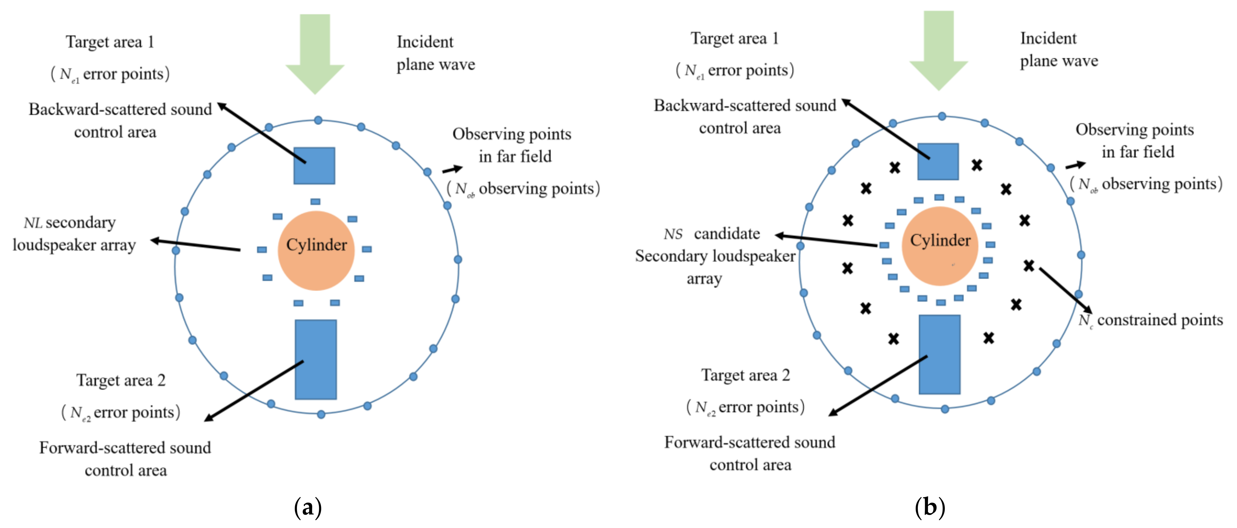
As shown in Figure 1a, one plane wave is incident, secondary loudspeakers are uniformly placed at a distance of from the cylinder, error points are placed in the backward-scattered sound control area of the cylinder that is denoted as target area 1, error points are placed in the forward-scattered sound control area of the cylinder that is denoted as target area 2, and observing points are uniformly placed at a distance of from the cylinder that is denoted as far-field observation area. The scattered sound pressure matrix of the error area (including target area 1 and target area 2) is expressed as:
where is the matrix (dimension ) of scattered acoustic transfer functions of target area 1 when one plane wave is incident, is the matrix (dimension ) of scattered acoustic transfer functions of target area 2 when one plane wave is incident, and is the strength vector (dimension ) of one incident plane wave.
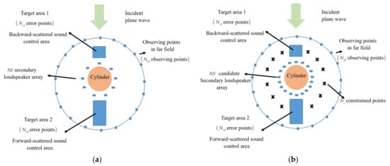
Figure 1.
Schematic of: (a) the RLS algorithm with the uniformly placed secondary loudspeakers; and (b) the new algorithm. The black crosses denote the constraint points.
When secondary sources are activated, the sound pressure matrix of the error area (including target area 1 and target area 2) can be written as:
where is the matrix (dimension ) of transfer functions from the uniformly placed secondary loudspeakers to target area 1, is the matrix (dimension ) of transfer functions from the uniformly placed secondary loudspeakers to target area 2, and is the strength vector (dimension ) of the secondary loudspeakers.
The RLS algorithm [14,20] using uniformly placed secondary loudspeakers aims to minimize the sound pressure in the target area under the premise that the secondary loudspeaker power is constrained . is the maximum allowable power of the secondary loudspeakers, and the cost function of the RLS algorithm is given by:
where is the regularization parameter. By setting the partial derivative of Equation (5) with respect to to zero, the solution to Equation (5) can be written as:
where , and is an identity matrix. After calculating the secondary loudspeaker strength vector with the initialized regularization parameter , if the power constraint condition is not satisfied, is increased until the condition is satisfied [18,26].
3. Proposed CLASSO-RLS Method for Multi-Zone Active Noise Control of the Scattered Sound from an Infinite Rigid Cylinder
As shown in Figure 1b, one plane wave is incident, candidate secondary loudspeakers are uniformly placed at a distance of from the cylinder, and constraint points are uniformly placed between the two target areas. To promote sparsity of the strength vector of the secondary loudspeakers and suppress the sound amplification of the constraint points, the CLASSO-RLS algorithm adds the -norm and the noise reduction constraint of the constraint points to the cost function of the RLS algorithm. The cost function of the CLASSO-RLS algorithm can be expressed as:
where is the matrix (dimension ) of transfer functions from the candidate secondary loudspeakers to target area 1, is the matrix (dimension ) of transfer functions from the candidate secondary loudspeakers to target area 2, is the strength vector (dimension ) of candidate secondary loudspeakers, denotes the noise reduction of the constraint points, and is the maximum noise reduction of the constraint points under a certain condition, which is defined in detail below. The sparse penalty parameter regulates the number of non-zero entries of [14]; the larger sparse penalty parameter results in fewer non-zero entries. The CLASSO-RLS algorithm selects optimized secondary loudspeakers from candidate secondary loudspeakers.
The CLASSO-RLS algorithm ensures a relatively large noise reduction in the target area as well as at the constraint points when selecting the sparse penalty parameter . The maximum noise reduction in the target area corresponds to a particular sparse penalty parameter. A small value of noise reduction will be neglected in this paper, so that several sparse penalty parameters corresponding to relatively large noise reduction can be obtained within a certain noise reduction range . Subsequently, the parameter with the largest noise reduction at the constraint points is selected as the final sparse penalty parameter . The detailed procedure for selecting is as follows:
Step 1: is the possible sparse penalty value and possible sparse penalty parameters are selected evenly in the selected value interval to form the possible sparse penalty value set (dimension ).
Step 2: Using the CVX toolbox [27] to solve Equation (7) and obtain the solution , the secondary loudspeakers with the largest amplitude in are selected as the chosen secondary loudspeakers for each . Equation (6) is used to calculate the strength vector (dimension ) of the chosen secondary loudspeakers , and calculate the target area noise reduction :
where is the matrix (dimension ) of transfer functions from the chosen secondary loudspeakers to the target area for . The calculation of the constraint point noise reduction is carried out using:
where is the scattered sound matrix (dimension ) of the constraint points, is the transfer function matrix (dimension ) from the chosen secondary loudspeakers to the constraint points for , and is the transfer function matrix (dimension ) from the candidate secondary loudspeakers to the constraint points; is selected from .
Here, the target area noise reduction set (dimension ) and the constraint point noise reduction set (dimension ) are formed. An important point of consideration after solving Equation (7) is the number of non-zero entries of . If this is less than , step 2 can be concluded.
Step 3: Let ; is a small value of noise reduction artificially defined and in this paper . By iterating through the target area noise reduction set , if , the corresponding is selected to form the alternative parameter set of values (dimension ) and the corresponding constraint point noise reduction is selected to form the set of values (dimension ).
Step 4: Let ; the corresponding to the maximum constraint point noise reduction is selected as the final sparse penalty parameter .
The CLASSO-RLS algorithm is divided into two stages. In the first stage, the value of is selected and the optimized secondary loudspeakers are obtained by solving Equation (7) using the CVX toolbox. In the second stage, the strength vector of the optimized secondary loudspeakers is solved using Equation (6). The complete computational description of the CLASSO-RLS algorithm is summarized in Algorithm 1. The main symbols are introduced in Table A1 in Appendix A.
| Algorithm 1. The CLASSO-RLS algorithm |
| Input: the matrix of scattered acoustic transfer functions of error points in target area 1 . |
| Input: the matrix of scattered acoustic transfer functions of error points in target area 2 . |
| Input: the matrix of scattered acoustic transfer functions of constraint points . |
| Input: the matrix of transfer functions from candidate secondary loudspeakers to error points in target area 1 . |
| Input: the matrix of transfer functions from candidate secondary loudspeakers to error points in target area 2 . |
| Input: the matrix of transfer functions from candidate secondary loudspeakers to conatraint points . |
| Input: the strength vector of one incident plane wave . |
| Output: the strength vector of optimized secondary loudspeakers . |
| Step 1: Select possible parameters evenly in the selected value interval to form the possible sparse penalty value set . |
| Step 2: Initialize the target area noise reduction set and the constraint point noise reduction set , so that their elements are 0. |
| Step 3: for . |
| , Use the CVX toolbox to solve Equation (7), the secondary loudspeakers |
| with the largest amplitude in are selected. |
| if |
| Use Equation (6) to calculate the strength vector of the chosen secondary loudspeakers |
| , use Equations (8) and (9) to calculate the target area noise reduction |
| and the constraint point noise reduction . |
| else |
| Skip to Step 4. |
| end if |
| Update the target area noise reduction set and the constraint point noise reduction set . |
| end for |
| Step 4: Obtain the maximum target area noise reduction . |
| Step 5: Initialize the alternative sparse penalty parameter set and the alternative constraint point noise reduction set , so that their elements are 0. Initialize a small value of noise reduction . |
| Step 6: for |
| if |
| Update the alternative sparse penalty parameter set and the alternative con-straint |
| point noise reduction set . |
| end if |
| end for |
| Step 7: Obtain the maximum constraint point noise reduction . |
| Step 8: Select the sparse penalty parameter corresponding to as the final sparse penalty parameter . |
| Step 9: Calculate the strength vector of optimized secondary loudspeakers using Equation (6). |
In this paper, the proposed CLASSO-RLS algorithm is compared with the RLS algorithm and the previous LASSO-RLS algorithm [14,15,16,17,20]. The LASSO-RLS algorithm often selects sparse penalty parameter using cross-validation techniques [14]. When secondary loudspeakers are chosen, the sparse penalty parameter can be selected in two ways. The first approach [14] is to assign the empirical value advocated in reference [28] to the sparse penalty parameter, and subsequently use the BCD algorithm [14] to solve Equation (7) and obtain the solution . Consequently, the secondary loudspeakers with the largest intensity values are selected as the optimized secondary loudspeakers. In the simulation, the first approach is called LASSO-RLS- method. The second method [20] is to increase and use the BCD method to solve Equation (7) until the number of non-zero entries in the strength vector of the optimized secondary loudspeakers is . Finally, the secondary loudspeakers are selected as the optimized secondary loudspeakers. In the simulation, this method is called the LASSO-RLS- algorithm. Neither the LASSO-RLS- method nor LASSO-RLS- algorithm have constraint points, which is the biggest difference to the proposed CLASSO-RLS algorithm. Both the LASSO-RLS- method and LASSO-RLS- algorithm have two stages. In the first stage, optimized secondary loudspeakers are selected from candidate secondary loudspeakers. In the second stage, is solved using Equation (6).
4. Simulation Results and Discussion
In this section, the simulation results of the proposed CLASSO-RLS algorithm, LASSO-RLS- method [14], LASSO-RLS- [20] method, and the RLS [14] algorithm using uniformly placed loudspeakers(called Uni-RLS algorithm) are compared.
4.1. Simulation Parameter Setting and Criteria of the Control Performance
In this 2D simulation, the primary sources are single-frequency plane waves with frequencies ranging from 400 Hz to 1100 Hz at a frequency interval of 100 Hz. The source strength of the primary field was and the strength vector (dimension ) of one incident plane wave was . The maximum power of the secondary loudspeakers was and the speed of sound was considered as . Target area 1 is set in the region of the backward-scattered sound, which is a square area with 169 uniformly distributed error points. Target area 2 is set in the forward-scattered sound region, which is a rectangular area with 325 evenly distributed error points. The spacing between the error points was and the radius of the cylinder was . The infinite line of monopoles is treated as a secondary loudspeaker. Eight secondary loudspeakers were placed uniformly around the cylinder at a distance of from the cylinder surface in Figure 1a. Eight optimized placed secondary loudspeakers were selected from 64 uniformly placed candidate secondary loudspeakers at a distance of from the cylinder surface in Figure 1b. Thirty-two constraint points were placed uniformly between target area 1 and target area 2 at a distance of from the cylinder surface in Figure 1b. To observe the noise reduction in the far field, 360 uniformly placed far-field observing points were located at a distance of from the center of the cylinder. To observe the noise reduction in the target area, 63,001 near-field observing points were evenly distributed in a square area in the x-y plane centered at the center of the cylinder; the spacing between the near-field observing points was . The noise reduction for one observing point is defined as:
where and are the sound pressures before and after the active noise control for one observing point, respectively. The noise reduction for the entire target area can be described as:
where is the ratio of the squared sum of the sound pressure before and after active noise control for 494 error points, is the sound pressure matrix (dimension ) for the error points before noise control and is the sound pressure matrix (dimension ) for the error points after noise control. Similarly, the noise reduction in target area 1 , the noise reduction in target area 2 , and the noise reduction in the far-field observation area can be computed as:
where is the ratio of the squared sum of the sound pressure before and after noise control for the 169 error points in target area 1, and is the ratio of the squared sum of the sound pressure before and after noise control for the 325 error points in target area 2. is the ratio of the squared sum of the sound pressure before and after noise control for 360 observing points in the far-field observation area.
4.2. Simulation Results of the Scattered Sound Field and the Loudspeaker Placement for Each Method
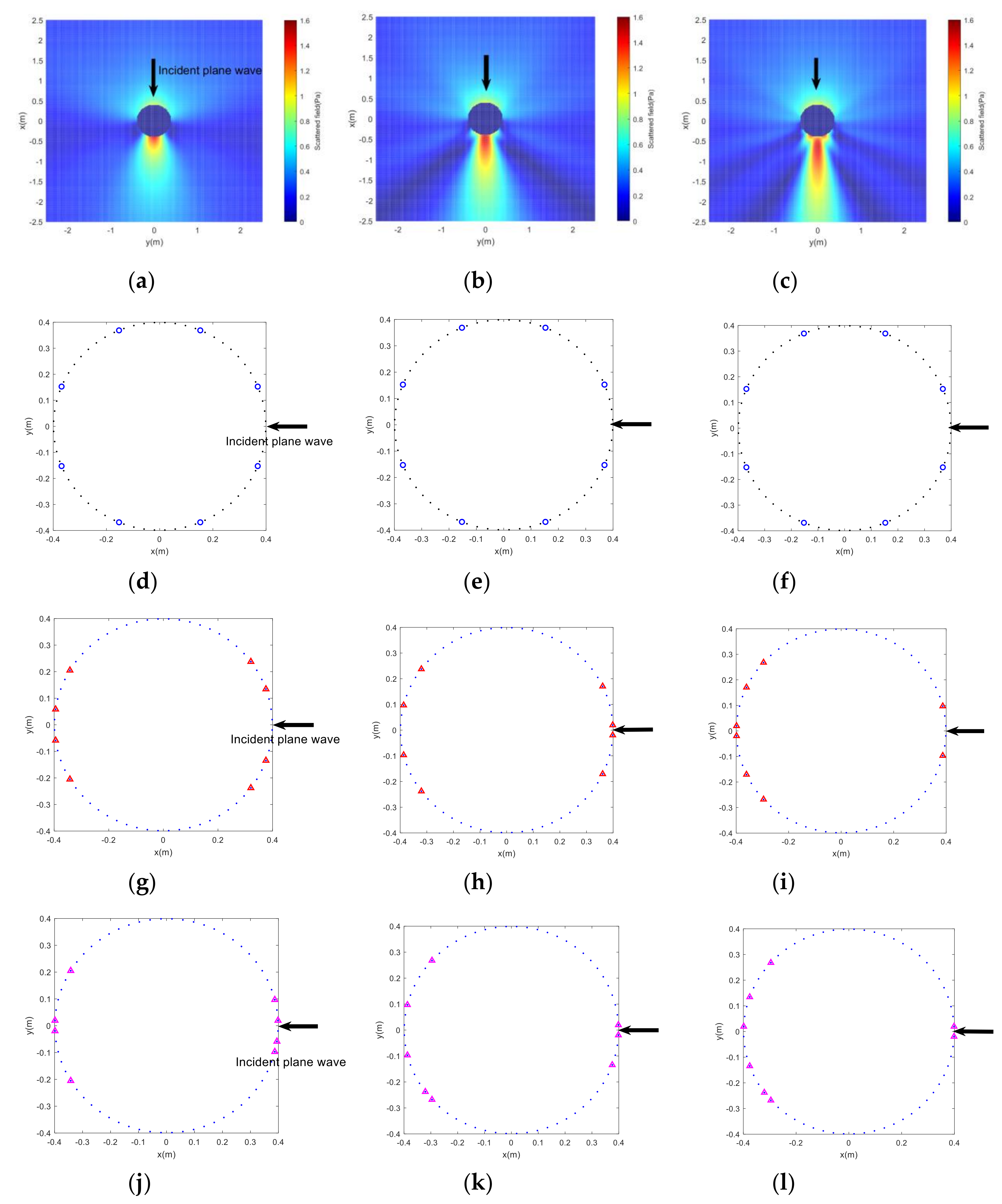
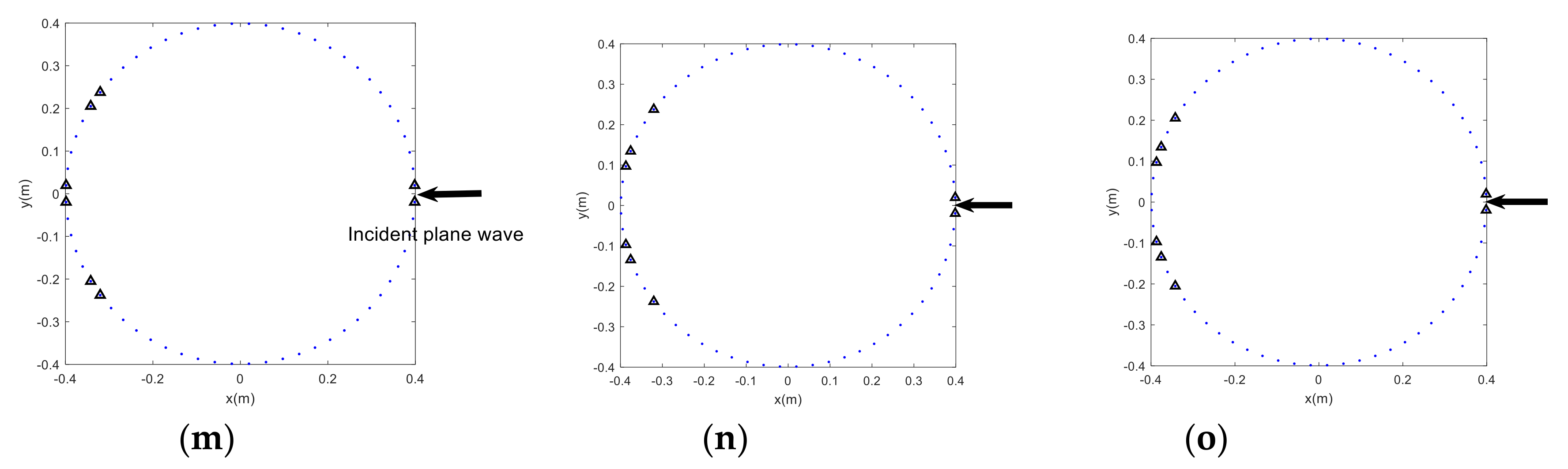
For the first simulation, the sound pressure amplitude of the scattered sound field and the results of the selected loudspeaker placement for each method from 400 Hz to 1000 Hz are shown in Figure 2. The first row shows scattered sound fields from 400 Hz to 1000 Hz, the second row shows Uni-RLS-based placement, the third row shows CLASSO-RLS-based placement, the fourth row shows LASSO-RLS--based placement, and the fifth row shows LASSO-RLS--based placement.
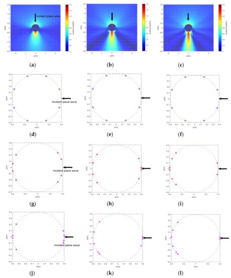
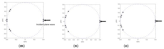
Figure 2.
Scattered sound field and the results of loudspeaker placement for each method from 400 Hz to 1000 Hz: (a) scattered sound field of the 400 Hz primary source; (b) scattered sound field of the 700 Hz primary source; (c) scattered sound field of the 1000 Hz primary source; (d) Uni-RLS (400 Hz); (e) Uni-RLS (700 Hz); (f) Uni-RLS (1000 Hz); (g) CLASSO-RLS (400 Hz); (h) CLASSO-RLS (700 Hz); (i) CLASSO-RLS (1000 Hz); (j) LASSO-RLS- (400 Hz); (k) LASSO-RLS- (700 Hz); (l) LASSO-RLS- (1000 Hz); (m) LASSO-RLS- (400 Hz); (n) LASSO-RLS- (700 Hz); and (o) LASSO-RLS- (1000 Hz).
Figure 2a–c shows that scattered sound power is mainly distributed in the forward-scattered sound area (in the negative half-axis of the x-axis) and the backward-scattered sound area (in the positive half-axis of the x-axis). The amplitude of the forward-scattered sound increases with increasing frequency, and the region of forward scattered sound becomes larger along the negative half-axis of the x-axis.
Figure 2d–f shows the uniformly placed secondary loudspeakers and the distribution of the secondary loudspeakers doesn’t change with increasing frequency. Figure 2g–i shows that the selected loudspeakers of the proposed CLASSO-RLS algorithm are mainly distributed in the forward region of the cylinder (near the region of the forward-scattered sound) and the backward region of the cylinder (near the region of the backward-scattered sound). As the frequency increases, there are more secondary loudspeakers in the forward region and the secondary loudspeaker distribution in the backward region becomes more concentrated.
Figure 2j–o illustrates that the selected loudspeakers of LASSO-RLS- method and those of the LASSO-RLS- method are mainly distributed in the forward and backward regions of the cylinder. The distribution of the secondary loudspeakers changes with increasing frequency. Compared to the CLASSO-RLS method, there are more secondary loudspeakers in the forward region and the distribution of the secondary loudspeakers in the backward region is more concentrated.
4.3. Simulation Results of the Control Performance for Each Method at 700 Hz
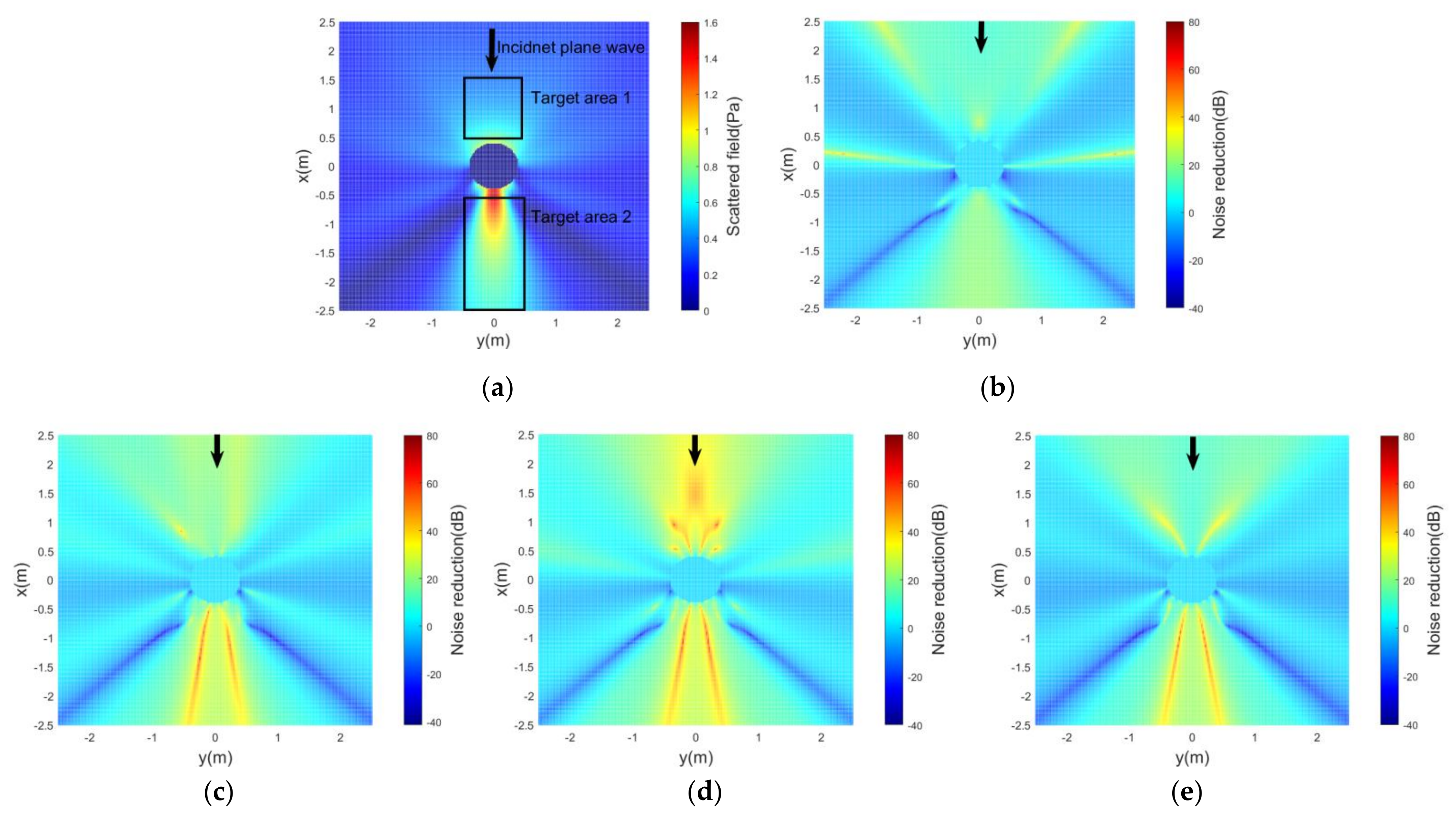
In the second simulation, the noise reduction of 63,001 near-field observing points in a square area can be calculated using Equation (10). The scattered sound field of the 700 Hz primary source and the noise reduction effects of the proposed CLASSO-RLS algorithm, the LASSO-RLS- method, the LASSO-RLS- method and the Uni-RLS algorithm at 700 Hz are shown in Figure 3.
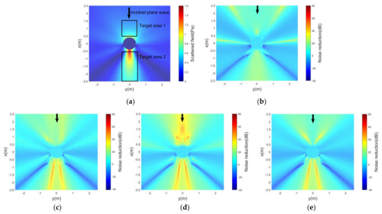
Figure 3.
Scattered sound field and the control performance for each method at 700 Hz: (a) scattered sound field of the 700 Hz primary source; (b) control performance of the Uni-RLS algorithm(700 Hz); (c) control performance of the LASSO-RLS- algorithm (d) control performance of the proposed CLASSO-RLS algorithm (700 Hz); and (e) control performance of the LASSO-RLS- algorithm (700 Hz).
Figure 3a shows that scattered sound power is mainly distributed in the forward-scattered sound area (the target area 2) and the backward-scattered sound area (the target area 1). The goal of the noise control is to obtain large noise reduction in these two areas.
As seen in Figure 3b, there is small noise reduction in two target areas. As shown in Figure 3c–e, compared to the Uni-RLS method, there are larger noise reductions in two target areas using the three secondary loudspeaker-optimized placement algorithms. Figure 3b–e illustrate that the reduction performance and size of the noise reduction areas of all three secondary loudspeaker-optimized placement algorithms are better than that of the Uni-RLS algorithm. The noise reduction of the entire error points in two target areas (calculated by Equation (11)) of the Uni-RLS algorithm, and the proposed CLASSO-RLS algorithm, LASSO-RLS- method, and the LASSO-RLS- method are 13 dB, 27 dB, 20 dB, and 16 dB, respectively. The poor performance of the Uni-RLS algorithm is due to the placement of the secondary loudspeakers at locations that are less critical (Figure 2e), such that the power of the secondary loudspeakers is not fully utilized. However, the secondary loudspeakers of the three optimized algorithms are placed at more important locations (Figure 2h,k,n) that are closer to the forward-scattered and backward-scattered target areas, such that the cancellation of the scattered sound field is better.
4.4. Simulation Results of the Noise Reduction for Each Method from 400 Hz to 1100 Hz
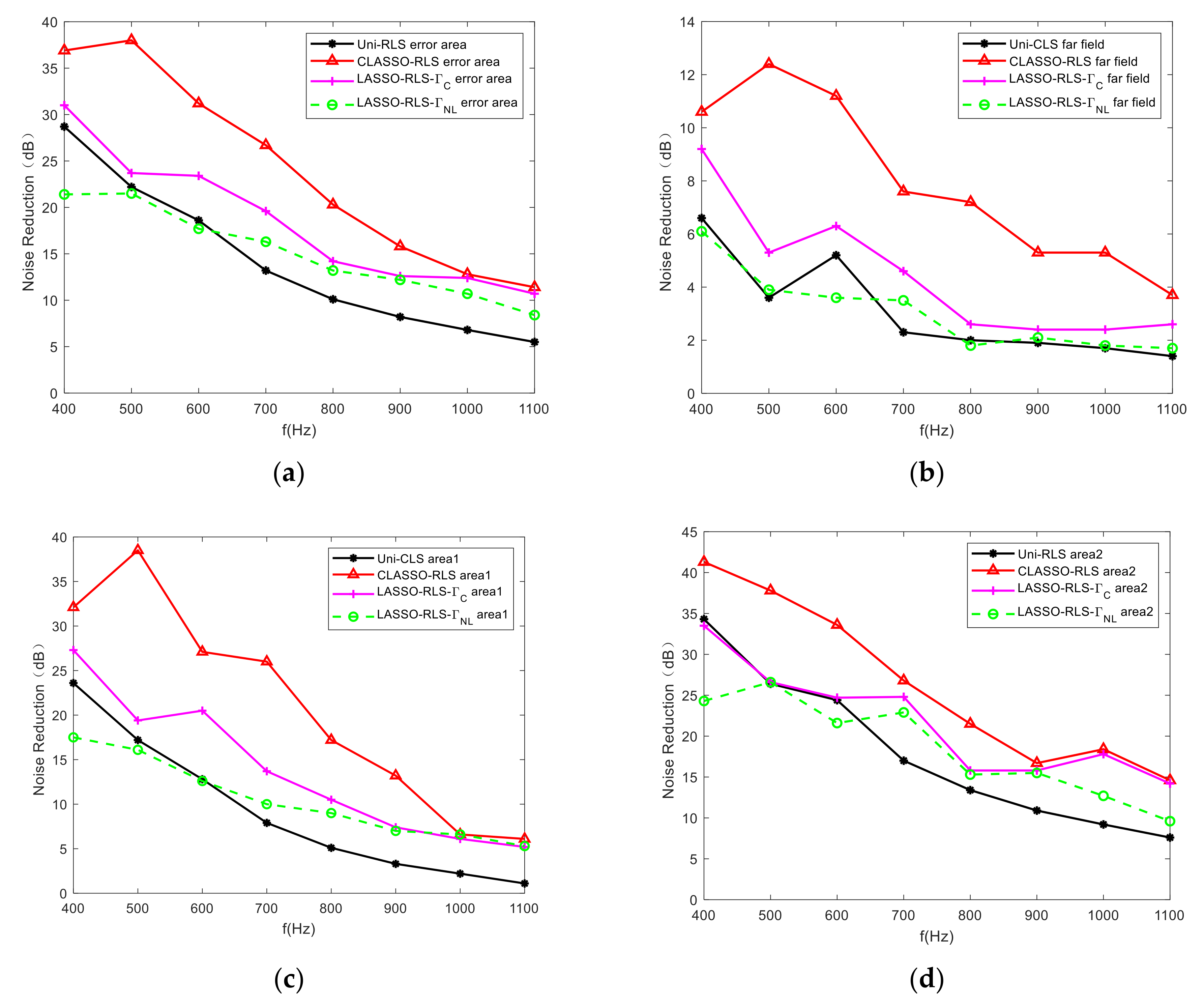
In the third simulation, the noise reduction of the entire error points , the noise reduction of the error points in target area 1 , the noise reduction of the error points in target area 2 , and the noise reduction of the far-field observing points for each method can be calculated using Equations (11)–(14). Figure 4a shows for each method, Figure 4b shows for each method, Figure 4c shows for each method, and Figure 4d shows for each method. The frequencies range from 400 Hz to 1100 Hz at a frequency interval of 100 Hz.
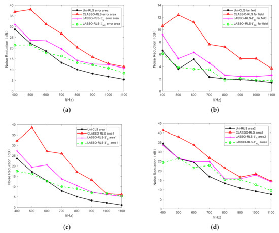
Figure 4.
Comparisons of the noise reduction for each method from 400 Hz to 1100 Hz: (a) the comparison of the noise reduction in the target area; (b) the comparison of the noise reduction in the far-field observing area; (c) the comparison of the noise reduction in the target area 1; and (d) the comparison of the noise reduction in the target area 2.
As shown in Figure 4, the noise reduction of each algorithm in the entire target area, target area 1, target area 2, and far-field observation area decreased with increasing frequency. Figure 4a illustrates that from 700 to 1100 Hz, the noise reduction of the three optimized algorithms in the entire target area is 2–13 dB greater than that of the Uni-RLS algorithm because the under-sampling issue of the uniformly placed secondary loudspeakers becomes gradually critical as the frequency increases. In contrast, the secondary loudspeaker spacing of the three optimized algorithms changes with increasing frequency. This provides better cancellation of the scattered sound field, resulting in improved noise reduction performance. Among the three optimized algorithms, the proposed CLASSO-RLS algorithm outperforms the other algorithms. From 400 Hz–1100 Hz, the proposed strategy gains a 5 dB–16 dB reduction performance advantage in the target area compared to the Uni-RLS algorithm.
As for the noise reduction performance in the far-field observation area, Figure 4b illustrates that the noise reduction of the proposed CLASSO-RLS algorithm is better than that of the other methods from 400 Hz–1100 Hz because of the addition of the constraint points. The secondary loudspeaker selection process of the CLASSO-RLS algorithm considers the noise reduction of the constraint points and the noise reduction of the entire target area. Thus, the noise reduction performance is better in the direction where the constraint points and the error points are located, and the noise reduction at the far-field observing points is also larger.
As shown in Figure 4c, the CLASSO-RLS algorithm achieves a noise reduction in target area1 that is 5–22 dB greater than that in the other two optimal methods from 400 Hz to 900 Hz. This is because the LASSO-RLS- and the LASSO-RLS- methods have fewer secondary loudspeakers distributed in the backward region of the cylinder compared to the CLASSO-RLS algorithm, and the distribution of the secondary loudspeakers is too concentrated to effectively cancel the scattered acoustic field.
Figure 4d illustrates that the CLASSO-RLS algorithm achieves better noise reduction in target area 2 compared to the other methods, because the change in the distribution of the selected secondary loudspeakers in the forward region more effectively matches the change in the wavelength of the sound as the frequency increases, leading to a better cancellation of the scattered sound field.
4.5. Simulation Results of the Control Perormance in Far Field for Each Method
In the fourth simulation, a comparison of the directivity for each method before and after active noise control at far-field observing points from 400 Hz to 1000 Hz is performed. As seen in Figure 1, 360 uniformly placed far-field observing points were located at a distance of from the center of the cylinder (the radius of the cylinder was ). Before active noise control, the sound pressure for one far-field observing point can be calculated by . The source strength of the primary field is . The scattered acoustic transfer function at one far-field observing point can be calculated using Equation (1). After active noise control, the sound pressure for one far-field observing point can be calculated by . The source strength vector (dimension ) of the selected secondary loudspeakers is calculated by each method introduced in Section 2 and Section 3. The matrix (dimension ) of the transfer functions form selected secondary loudspeakers to one far-field observing point can be obtained using Equation (2).
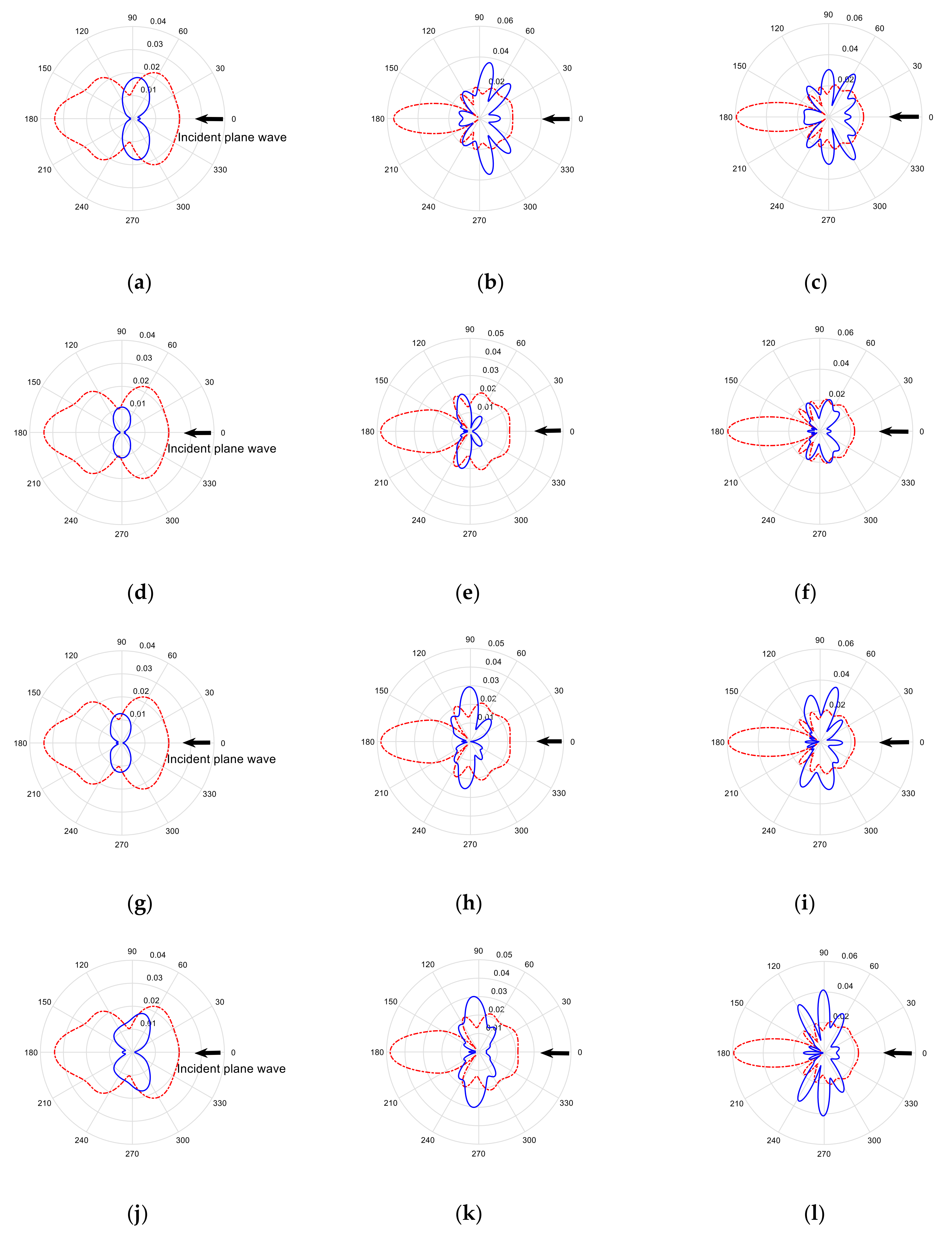
The absolute values of the sound pressure before active noise control for 360 far-field observing points are shown as the red dotted lines in Figure 5. The absolute values of the sound pressure after active noise control for 360 far-field observing points are shown as the blue solid lines in Figure 5. The frequencies range from 400 Hz to 1000 Hz at a frequency interval of 300 Hz. The first row shows the directivity patterns for Uni-RLS algorithm, the second row shows the directivity patterns for CLASSO-RLS algorithm, the third row shows the directivity patterns for LASSO-RLS- algorithm, and the fourth row shows the directivity patterns for LASSO-RLS- algorithm.
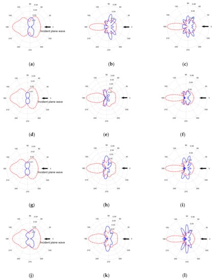
Figure 5.
Comparison of the directivity for each method before and after active noise control at far-field observing points from 400 Hz to 1000 Hz: (a) Uni-RLS (400 Hz); (b) Uni-RLS (700 Hz); (c) Uni-RLS (1000 Hz); (d) CLASSO-RLS (400 Hz); (e) CLASSO-RLS (700 Hz); (f) CLASSO-RLS (1000 Hz); (g) LASSO-RLS- (400 Hz); (h) LASSO-RLS- (700 Hz); (i) LASSO-RLS- (1000 Hz); (j) LASSO-RLS- (400 Hz); (k) LASSO-RLS- (700 Hz); and (l) LASSO-RLS- (1000 Hz). The red dotted line corresponds to the control off and the blue solid line corresponds to the control on.
As seen in Figure 5, in the directions where the target areas are located, the blue solid line is smaller than the red dotted line for each method. It illustrates that all algorithms have good noise reduction in the directions of the forward-scattered sound and backward-scattered sound target areas. However, as shown in Figure 5a–c,g–l, in the directions with an angle of 90° from the incident direction, the blue solid lines are bigger than the red dotted lines. It illustrates that Uni-RLS algorithm, LASSO-RLS- method and LASSO-RLS- method exhibit sound amplification after active noise control in the two directions and the sound amplification becomes more apparent with increasing frequency. This is due to the fact that as the frequency increases, the secondary loudspeakers need more power to provide good noise reduction in the target areas. However, as the power increases, the secondary loudspeakers produce larger sound amplification outside the target areas.
In contrast, as shown in Figure 5d–f, in the directions with an angle of 90° from the incident direction, the blue solid lines and the red dotted lines have approximately the same values. It illustrates that the proposed CLASSO-RLS algorithm exhibits negligible sound amplification after active noise control in the two directions. This is because the CLASSO-RLS algorithm places constraint points in the non-error areas (Figure 1b). Moreover, the noise reduction of the constraint points is considered in the process of selecting secondary loudspeakers to reduce the noise at the constraint points as much as possible under a stipulated condition, thereby effectively suppressing the sound amplification in the direction where the constraint points are located.
5. Conclusions
For the multi-zone active noise control of scattered sound from infinite rigid cylinders, an active control strategy combining the LASSO algorithm with constraint points and the RLS algorithm is proposed in this paper. Simulation results show that the new method achieves a 5 dB–16 dB reduction performance advantage in the target area compared to the RLS algorithm employing uniformly placed loudspeakers from 400 Hz to 1100 Hz. Additionally, the noise reduction performance of the new method is better than that of the previous LASSO algorithm. The new method improves the control performance of the scattered sound control to render the scattered object invisible to the incident acoustic waves; it exhibits a larger noise reduction in the forward-scattered and backward-scattered sound target areas, with no significant sound amplification in the far field observation area. This is because the new method adds constraint points and considers both the noise reduction of the error points as well as that of the constraint points when selecting the optimal secondary loudspeakers.
The proposed control algorithm has an important application in scattered sound control: it can achieve large noise reduction in multiple zones of the scattered sound while suppressing the sound amplification outside the target area. The new algorithm has a lower computational complexity than that of the RLS algorithm with uniform placement of secondary loudspeakers. This is because the RLS algorithm with uniformly placed secondary loudspeakers needs more loudspeakers to achieve the same noise reduction effect, which increases the computational complexity in the calculation of the loudspeaker strength. In future work, the multi-zone control algorithm for finite-length cylindrical scattered objects will be investigated and their practical control effect will be verified.
Author Contributions
Conceptualization, Y.F. and X.W.; methodology, Y.F.; software, Y.F.; validation, Y.F., M.W. and X.W.; formal analysis, Y.F.; investigation, Y.F. and X.C.; resources, J.Y.; data curation, Y.F. and X.C.; writing—original draft preparation, Y.F. and X.W.; writing—review and editing, Y.F., X.W., J.Y., X.C. and M.W.; visualization, Y.F.; supervision, J.Y.; project administration, X.W. and J.Y.; funding acquisition, X.W. and J.Y. All authors have read and agreed to the published version of the manuscript.
Funding
This research was funded by the National Natural Science Foundation of China (grant 11804365 and 11804368).
Institutional Review Board Statement
Not applicable.
Informed Consent Statement
Not applicable.
Data Availability Statement
The data presented in this study are available on request from the corresponding author.
Conflicts of Interest
The authors declare no conflict of interest.
Appendix A
The main symbols in this paper are shown in Table A1.

Table A1.
Main symbols in the simulation.
Table A1.
Main symbols in the simulation.
| Symbol | Meaning |
|---|---|
| The number of error points in target area 1 | |
| The number of error points in target area 2 | |
| The number of far-field observing points | |
| The number of constraint points | |
| The number of candidate secondary loudspeakers | |
| The number of the selected secondary loudspeakers | |
| The matrix (dimension ) of scattered acoustic transfer functions of target area 1 when one plane wave is incident | |
| The matrix (dimension ) of scattered acoustic transfer functions of target area 2 when one plane wave is incident | |
| The strength vector(dimension ) of one incident plane wave | |
| The strength vector (dimension ) of the selected secondary loudspeakers. | |
| The maximum allowable power of the secondary loudspeakers | |
| The matrix (dimension ) of transfer functions from the uniformly placed secondary loudspeakers to target area 1 | |
| The matrix (dimension ) of transfer functions from the uniformly placed secondary loudspeakers to target area 2 | |
| The regularization parameter | |
| The matrix (dimension ) of transfer functions from the candidate secondary loudspeakers to target area 1 | |
| The matrix (dimension ) of transfer functions from the candidate secondary loudspeakers to target area 2 | |
| The sparse penalty parameter in CLASSO-RLS method | |
| The sparse penalty parameter in LASSO method | |
| The noise reduction of the entire error points when the sparse penalty is in CLASSO-RLS method | |
| The noise reduction of the constraint points when the sparse penalty is in CLASSO-RLS method | |
| The maximum noise reduction of the constraint points under a certain condition in CLASSO-RLS method | |
| The maximum noise reduction of the entire error points in CLASSO-RLS method | |
| A small value of noise reduction in CLASSO-RLS method | |
| The noise reduction of one observing point in criteria of the control performance | |
| The noise reduction of the entire error points in criteria of the control performance | |
| The noise reduction of the error points in target area 1 in criteria of the control performance | |
| The noise reduction of the error points in target area 2 in criteria of the control performance | |
| The noise reduction of the far-field observing points in criteria of the control performance | |
| The sound pressure before the active noise control for one observing point | |
| The sound pressure after the active noise control for one observing point | |
| The sound pressure before the active noise control for one far-field observing point | |
| The sound pressure after the active noise control for one far-field observing point |
References
- Jorden, C. Active control of scattered acoustic fields: Cancellation, reproduction and cloaking. J. Acoust. Soc. Am. 2016, 140, 1502–1512. [Google Scholar]
- Nelson, P.A.; Elliott, S.J. Active control of sound. Phys. Today 1993, 46, 75–76. [Google Scholar] [CrossRef]
- Kajikawa, Y.; Gan, W.S.; Kuo, S.M. Recent advances on active noise control: Open issues and innovative applications. Apsipa Trans. Signal Inf. Process. 2012, 1, e3. [Google Scholar] [CrossRef] [Green Version]
- Han, N.; Qiu, X.; Feng, S. Active Control of Three-Dimension Impulsive Scattered Radiation Based on a Prediction Method. Mech. Syst. Signal Process. 2012, 30, 267–273. [Google Scholar] [CrossRef]
- Friot, E.; Bordier, C. Real-Time Active Suppression of Scattered Acoustic Radiation. J. Sound Vib. 2004, 278, 563–580. [Google Scholar] [CrossRef]
- Rafaely, B. Spherical Loudspeaker Array for Local Active Control of Sound. J. Acoust. Soc. Am. 2009, 125, 3006–3017. [Google Scholar] [CrossRef]
- Peleg, T.; Rafaely, B. Investigation of Spherical Loudspeaker Arrays for Local Active Control of Sound. J. Acoust. Soc. Am. 2011, 130, 1926–1935. [Google Scholar] [CrossRef] [PubMed]
- Liu, J.; Wang, X.; Wu, M.; Jun, Y. An active control strategy for the scattered sound field control of a rigid sphere. J. Acoust. Soc. Am. 2018, 144, EL52–EL58. [Google Scholar] [CrossRef]
- Baek, K.H.; Elliott, S.J. Natural Algorithms for Choosing Source Locations in Active Control Systems. J. Sound Vib. 1995, 186, 245–267. [Google Scholar] [CrossRef]
- Li, D.; Hodgson, M. Optimal Active Noise Control in Large Rooms Using a “Locally Global” Control Strategy. J. Acoust. Soc. Am. 2005, 118, 3653–3661. [Google Scholar] [CrossRef]
- Duke, C.R.; Sommerfeldt, S.D.; Gee, K.L.; Duke, C.V. Optimization of Control Source Locations in Free-Field Active Noise Control Using a Genetic Algorithm. Noise Control Eng. J. 2009, 57, 221–231. [Google Scholar] [CrossRef]
- Chen, G.S.; Bruno, R.J.; Salama, M. Optimal placement of active/passive members in truss structures using simulated annealing. AIAA J. 1991, 29, 1327–1334. [Google Scholar] [CrossRef]
- Yu, G.; Cheng, L. Location optimization of a long T-shaped acoustic resonator array in noise control of enclosures. J. Sound Vib. 2009, 328, 42–56. [Google Scholar] [CrossRef]
- Lilis, G.N.; Angelosante, D.; Giannakis, G.B. Sound Field Reproduction Using the Lasso. IEEE Trans. Audio Speech Lang. Process. 2010, 18, 1902–1912. [Google Scholar] [CrossRef]
- Radmanesh, N.; Burnett, I.S. Wideband Sound Reproduction in a 2D Multi-Zone System Using a Combined Two-Stage Lasso-LS Algorithm. In Proceedings of the 2012 IEEE 7th Sensor Array and Multichannel Signal Processing Workshop (SAM), Hoboken, NJ, USA, 17–20 June 2012; pp. 453–456. [Google Scholar]
- Radmanesh, N.; Burnett, I.S. Generation of Isolated Wideband Sound Fields Using a Combined Two-Stage Lasso-LS Algorithm. IEEE Trans. Audio Speech Lang. Process. 2013, 21, 378–387. [Google Scholar] [CrossRef]
- Radmanesh, N.; Burnett, I.S.; Rao, B.D. A Lasso-LS Optimization with a Frequency Variable Dictionary in a Multizone Sound System. IEEE/ACM Trans. Audio Speech Lang. Process. 2016, 24, 583–593. [Google Scholar] [CrossRef]
- Khalilian, H.; Bajic, I.V.; Vaughan, R.G. Loudspeaker Placement for Sound Field Reproduction by Constrained Matching Pursuit. In Proceedings of the 2013 IEEE Workshop on Applications of Signal Processing to Audio and Acoustics (WASPAA), New Paltz, NY, USA, 20–23 October 2013; pp. 1–4. [Google Scholar]
- Khalilian, H.; Bajic, I.V.; Vaughan, R.G. Towards optimal source placement for sound field reproduction. In Proceedings of the 2013 IEEE Workshop on International Conference on Acoustics, Speech and Signal Processing (ICASSP), Vancouver, BC, Canada, 26–31 May 2013; pp. 321–325. [Google Scholar]
- Khalilian, H.; Bajic, I.V.; Vaughan, R.G. Comparison of Loudspeaker Placement Methods for Sound Field Reproduction. IEEE/ACM Trans. Audio Speech Lang. Process. 2016, 24, 1364–1379. [Google Scholar] [CrossRef]
- Zhu, M.; Zhao, S. An Iterative Approach to Optimize Loudspeaker Placement for Multi-Zone Sound Field Reproduction. J. Acoust. Soc. Am. 2021, 149, 3462–3468. [Google Scholar] [CrossRef] [PubMed]
- Choi, J.W.; Kim, Y.H. Generation of an acoustically bright zone with an illuminated region using multiple sources. J. Acoust. Soc. Am. 2002, 111, 1695–1700. [Google Scholar] [CrossRef]
- Asano, F.; Suzuki, Y.; Swanson, D.C. Optimization of Control Source Configuration in Active Control Systems Using Gram–Schmidt Orthogonalization. IEEE Trans. Audio Speech Lang. Process. 1999, 7, 213–220. [Google Scholar] [CrossRef]
- Makris, N.C. A Spectral Approach to 3-D Object Scattering in Layered Media Applied to Scattering from Submerged Spheres. J. Acoust. Soc. Am. 1998, 104, 2015–2113. [Google Scholar] [CrossRef]
- Friot, E.; Bordier, C. A Free-field Experiment of Multichannel Control for Random Noise Coming from Uncorrelated Sources in an Anechoic Room. In Proceedings of the International Symposium on Active Control of Sound and Vibration (ACTIVE), Southampton, UK, 15–17 July 2002; pp. 221–230. [Google Scholar]
- Betlehem, T.; Withers, C. Sound Field Reproduction with Energy Constraint on Loudspeaker Weights. IEEE Trans. Audio Speech Lang. Process. 2012, 20, 2388–2392. [Google Scholar] [CrossRef]
- CVX: Matlab Software for Disciplined Convex Programming, Version 2.0 Beta. Available online: http://cvxr.com/cvx (accessed on 15 December 2018).
- Sardy, S.; Bruce, A.G.; Tseng, P. Block Coordinate Relaxation Methods for Nonparametric Wavelet Denoising. J. Comput. Graph. Statist. 2000, 9, 361–379. [Google Scholar]
Publisher’s Note: MDPI stays neutral with regard to jurisdictional claims in published maps and institutional affiliations. |
© 2021 by the authors. Licensee MDPI, Basel, Switzerland. This article is an open access article distributed under the terms and conditions of the Creative Commons Attribution (CC BY) license (https://creativecommons.org/licenses/by/4.0/).