
Quantifying Auditory Presence Using Electroencephalography


Abstract
:1. Introduction
1.1. Presence
1.2. Subjective Measurement
1.3. Objective Measurement
1.4. Summary
2. Materials and Methods
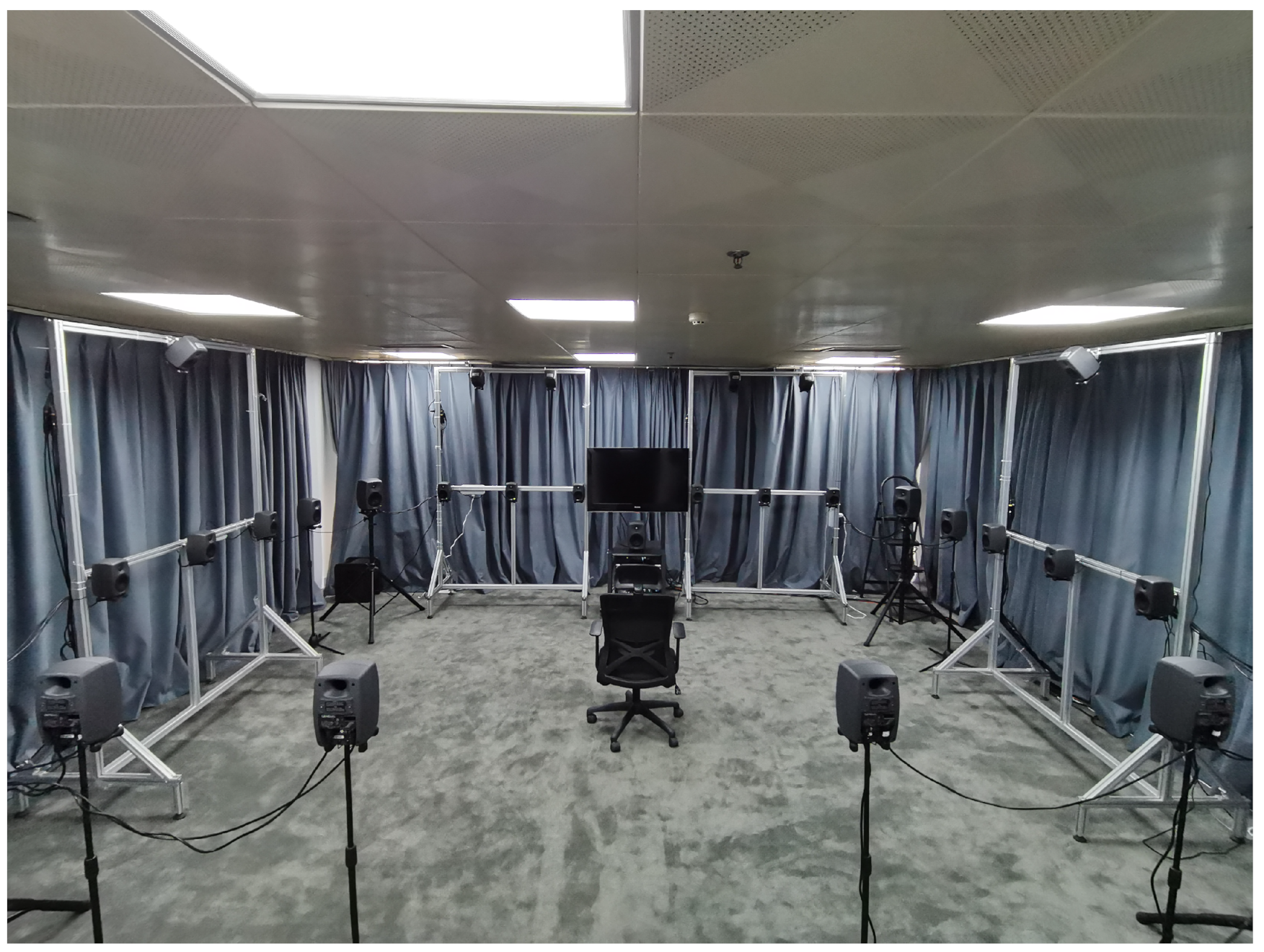
2.1. Program Selection and Listening Environment
2.2. Questionnaires
- Please rate your sense of being in the virtual environment on a scale of 0 to 10, where 10 represents your normal experience of being in a place;
- During your experience, did you often think to yourself that you were actually in the virtual environment? Please rate it on a scale of 0 to 10, where 10 represents you almost feel you were actually in the virtual environment;
- How well could you identify sounds? Please rate it on a scale of 0 to 10, where 10 represents you could clearly identify different kinds of sounds;
- How well could you localize sounds? Please rate it on a scale of 0 to 10, where 10 represents you could easily detect the location of each sound.
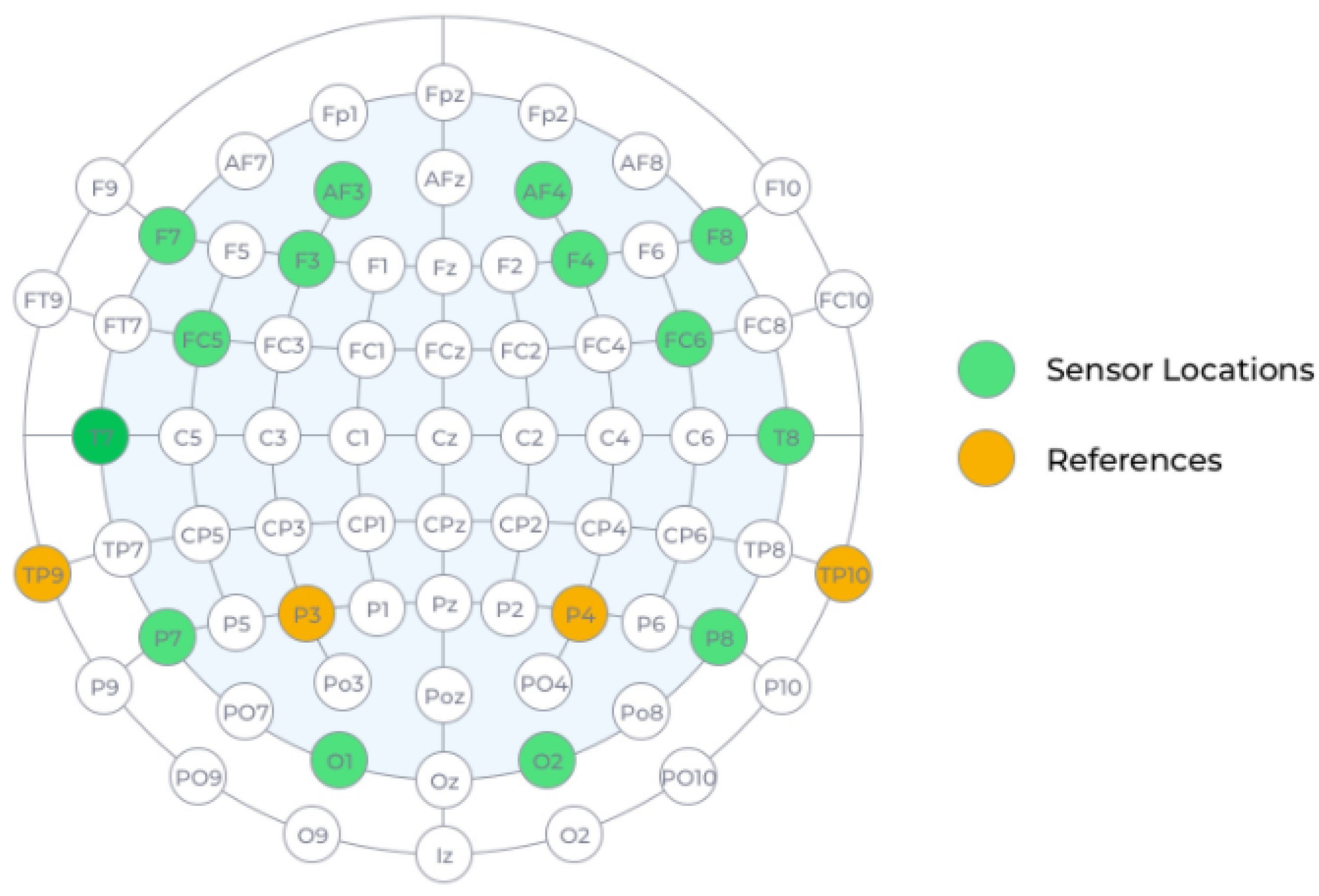
2.3. EEG Apparatus
2.4. Experiment Design
2.4.1. Experiment 1
2.4.2. Experiment 2
2.5. Signal Processing
3. Results
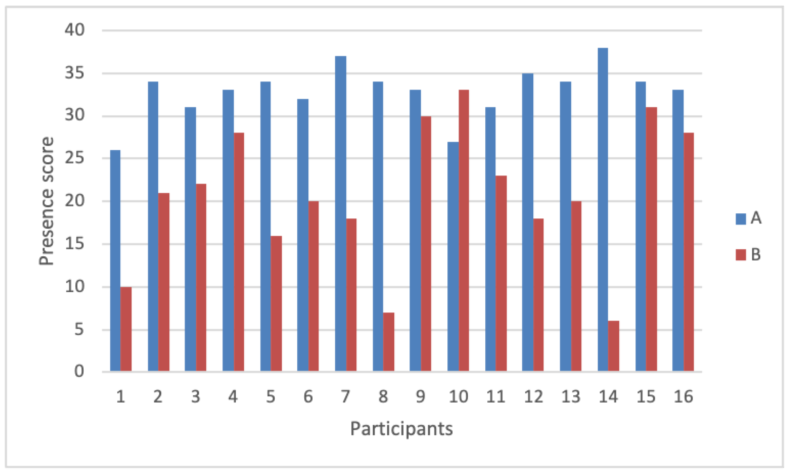
3.1. Experiment 1
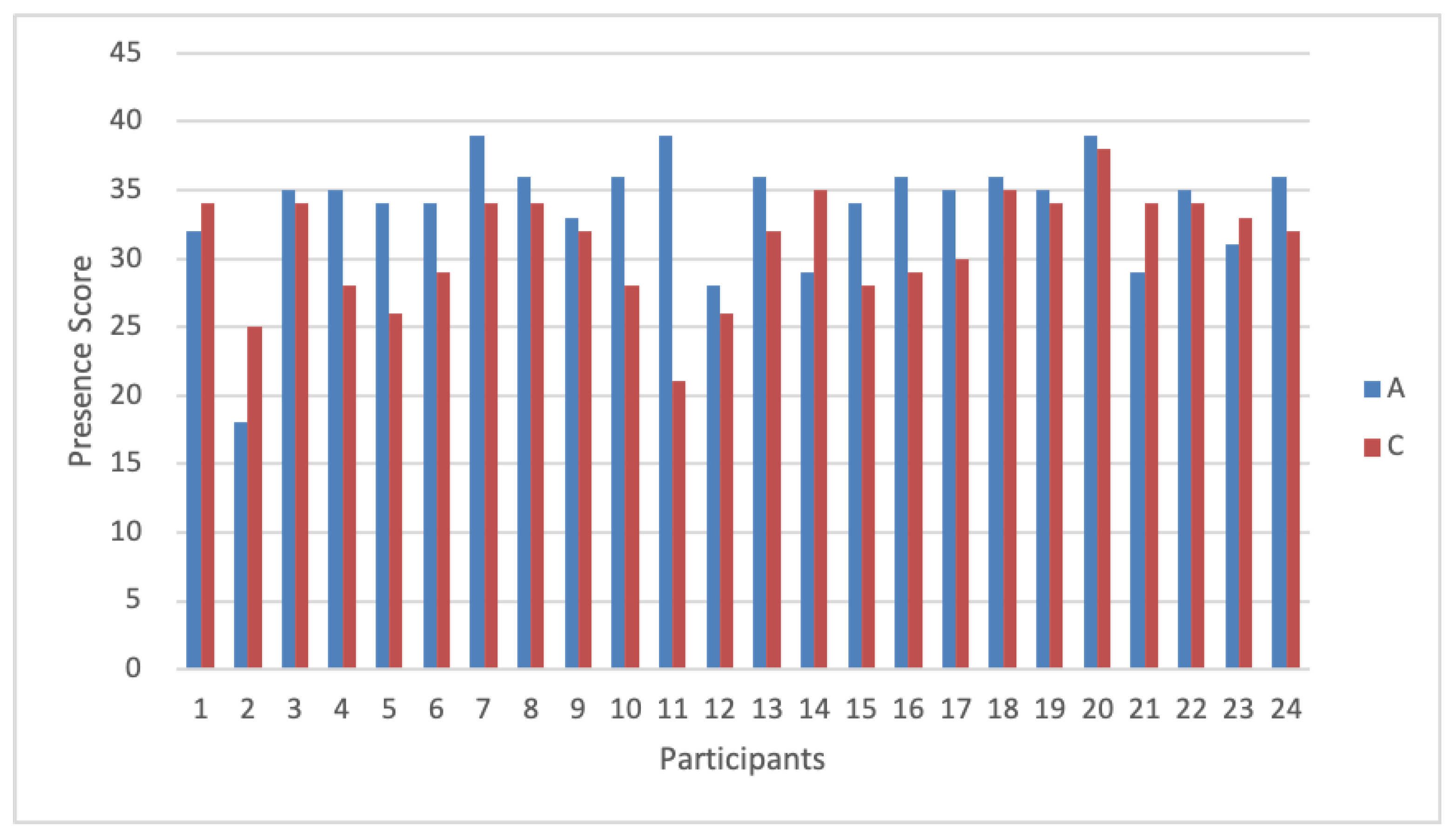
3.2. Experiment 2
4. Discussion
4.1. Post-Test Interview
4.2. T/B in Neuroscience
4.3. Correlation between Questionnaires and EEG Indices
5. Conclusions
Author Contributions
Funding
Institutional Review Board Statement
Informed Consent Statement
Data Availability Statement
Acknowledgments
Conflicts of Interest
Abbreviations
| EEG | electroencephalography |
| T/A | the power ratio of theta/alpha |
| T/B | the power ratio of theta/beta |
| T/AB | the power ratio of theta/(alpha+beta) |
| A/B | the power ratio of alpha/beta |
References
- Slater, M.; Usoh, M.; Steed, A. Depth of Presence in Virtual Environments. Presence Teleoperators Virtual Environ. 1994, 3, 130–144. [Google Scholar] [CrossRef]
- Witmer, B.G.; Singer, M.J. Measuring presence in virtual environments: A presence questionnaire. Presence Teleoperators Virtual Environ. 1998, 7, 225–240. [Google Scholar] [CrossRef]
- Patrick, E.; Cosgrove, D.; Slavkovic, A.; Rode, J.A.; Verratti, T.; Chiselko, G. Using a large projection screen as an alternative to head-mounted displays for virtual environments. In Proceedings of the SIGCHI conference on Human Factors in Computing Systems, The Hague, The Netherlands, 1–6 April 2000; pp. 478–485. [Google Scholar]
- Riva, G.; Davide, F.; IJsselsteijn, W.A. Being there: The experience of presence in mediated environments. In Being There: Concepts, Effects and Measurement of User Presence in Synthetic Environments; Ios Press: Amsterdam, The Netherlands, 2003; Volume 5. [Google Scholar]
- Agrawal, S.; Simon, A.; Bech, S.; BÆrentsen, K.; Forchhammer, S. Defining immersion: Literature review and implications for research on audiovisual experiences. AES J. Audio Eng. Soc. 2020, 68, 404–417. [Google Scholar] [CrossRef]
- Clemente, M.; Rodríguez, A.; Rey, B.; Alcañiz, M. Assessment of the influence of navigation control and screen size on the sense of presence in virtual reality using EEG. Expert Syst. Appl. 2014, 41, 1584–1592. [Google Scholar] [CrossRef]
- Dey, A.; Phoon, J.; Saha, S.; Dobbins, C.; Billinghurst, M. A Neurophysiological Approach for Measuring Presence in Immersive Virtual Environments. In Proceedings of the 2020 IEEE International Symposium on Mixed and Augmented Reality, ISMAR 2020, Porto de Galinhas, Brazil, 9–13 November 2020; pp. 474–485. [Google Scholar] [CrossRef]
- Hendrix, C.; Barfield, W. Presence in virtual environments as a function of visual and auditory cues. In Proceedings of the Virtual Reality Annual International Symposium ’95, Research Triangle Park, NC, USA, 11–15 March 1995; pp. 74–82. [Google Scholar]
- Hendrix, C.; Barfield, W. The sense of presence within auditory virtual environments. Presence Teleoperators Virtual Environ. 1996, 5, 290–301. [Google Scholar] [CrossRef]
- Rumsey, F.; Berg, J. Verification and correlation of attributes used for describing the spatial quality of reproduced sound. In Proceedings of the Audio Engineering Society Conference: 19th International Conference: Surround Sound-Techniques, Technology, and Perception, Schloss Elmau, Germany, 21–24 June 2001. [Google Scholar]
- Ozawa, K.; Chujo, Y.; Suzuki, Y.; Sone, T. Contents which yield high auditory-presence in sound reproduction. Kansei Eng. Int. 2002, 3, 25–30. [Google Scholar]
- Ozawa, K.; Ohtake, S.; Suzuki, Y.; Sone, T. Effects of visual information on auditory presence. Acoust. Sci. Technol. 2003, 24, 97–99. [Google Scholar] [CrossRef]
- Nicol, R.; Dufor, O.; Gros, L.; Rueff, P.; Farrugia, N. EEG measurement of binaural sound immersion. In Proceedings of the EAA Spatial Audio Signal Processing Symposium, Paris, France, 6–7 September 2019; pp. 73–78. [Google Scholar]
- Schwind, V.; Knierim, P.; Haas, N.; Henze, N. Using presence questionnaires in virtual reality. In Proceedings of the 2019 CHI Conference on Human Factors in Computing Systems, Glasgow, Scotland, UK, 4–9 May 2019; pp. 1–12. [Google Scholar]
- Witmer, B.G.; Jerome, C.J.; Singer, M.J. The factor structure of the Presence Questionnaire. Presence Teleoperators Virtual Environ. 2005, 14, 298–312. [Google Scholar] [CrossRef]
- Slater, M.; McCarthy, J.; Maringelli, F. The influence of body movement on subjective presence in virtual environments. Hum. Factors 1998, 40, 469–477. [Google Scholar] [CrossRef] [Green Version]
- Usoh, M.; Arthur, K.; Whitton, M.C.; Bastos, R.; Steed, A.; Slater, M.; Brooks, F.P., Jr. Walking > walking-in-place > flying, in virtual environments. In Proceedings of the 26th Annual Conference on Computer Graphics and Interactive Techniques, Los Angeles, CA, USA, 8–13 August 1999; pp. 359–364. [Google Scholar]
- Slater, M.; Steed, A. A virtual presence counter. Presence Teleoperators Virtual Environ. 2000, 9, 413–434. [Google Scholar] [CrossRef] [Green Version]
- Slater, M. How colorful was your day? Why questionnaires cannot assess presence in virtual environments. Presence 2004, 13, 484–493. [Google Scholar] [CrossRef]
- Sanchez-Vives, M.V.; Slater, M. From presence to consciousness through virtual reality. Nat. Rev. Neurosci. 2005, 6, 332–339. [Google Scholar] [CrossRef]
- Meehan, M.; Insko, B.; Whitton, M.; Brooks, F.P., Jr. Physiological measures of presence in stressful virtual environments. ACM Trans. Graph. (TOG) 2002, 21, 645–652. [Google Scholar] [CrossRef] [Green Version]
- Terkildsen, T.; Makransky, G. Measuring presence in video games: An investigation of the potential use of physiological measures as indicators of presence. Int. J. Hum. Comput. Stud. 2019, 126, 64–80. [Google Scholar] [CrossRef]
- Baumgartner, T.; Speck, D.; Wettstein, D.; Masnari, O.; Beeli, G.; Jäncke, L. Feeling present in arousing virtual reality worlds: Prefrontal brain regions differentially orchestrate presence experience in adults and children. Front. Hum. Neurosci. 2008, 2, 8. [Google Scholar] [CrossRef] [PubMed] [Green Version]
- Kober, S.E.; Kurzmann, J.; Neuper, C. Cortical correlate of spatial presence in 2D and 3D interactive virtual reality: An EEG study. Int. J. Psychophysiol. 2012, 83, 365–374. [Google Scholar] [CrossRef] [PubMed]
- Kober, S.E.; Neuper, C. Using auditory event-related EEG potentials to assess presence in virtual reality. Int. J. Hum. Comput. Stud. 2012, 70, 577–587. [Google Scholar] [CrossRef]
- Clemente, M.; Rodriguez, A.; Rey, B.; Alcañiz, M. Measuring presence during the navigation in a virtual environment using EEG. Stud. Health Technol. Inform. 2013, 191, 136–140. [Google Scholar]
- Abromavičius, V.; Gedminas, A.; Serackis, A. Detecting sense of presence changes in EEG spectrum during perception of immersive audiovisual content. In Proceedings of the 2017 Open Conference of Electrical, Electronic and Information Sciences (eStream), Vilnius, Lithuania, 27 April 2017; pp. 1–4. [Google Scholar]
- Lim, S.; Yeo, M.; Yoon, G. Comparison between concentration and immersion based on EEG analysis. Sensors 2019, 19, 1669. [Google Scholar] [CrossRef] [Green Version]
- Jap, B.T.; Lal, S.; Fischer, P.; Bekiaris, E. Using EEG spectral components to assess algorithms for detecting fatigue. Expert Syst. Appl. 2009, 36, 2352–2359. [Google Scholar] [CrossRef]
- Wen, T.Y.; Aris, S.A.M. Electroencephalogram (EEG) stress analysis on alpha/beta ratio and theta/beta ratio. Indones. J. Electr. Eng. Comput. Sci. 2020, 17, 175–182. [Google Scholar] [CrossRef] [Green Version]
- Sanei, S.; Chambers, J.A. EEG Signal Processing; John Wiley & Sons: Hoboken, NJ, USA, 2013. [Google Scholar]
- Donoghue, T.; Dominguez, J.; Voytek, B. Electrophysiological Frequency Band Ratio Measures Conflate Periodic and Aperiodic Neural Activity. bioRxiv 2020, 7, 1–14. [Google Scholar] [CrossRef] [PubMed]
- Chen, C.C.; Hsu, C.Y.; Chiu, H.W.; Hu, C.J.; Lee, T.C. Frequency power and coherence of electroencephalography are correlated with the severity of Alzheimer’s disease: A multicenter analysis in Taiwan. J. Formos. Med. Assoc. 2015, 114, 729–735. [Google Scholar] [CrossRef] [Green Version]
- Trammell, J.P.; MacRae, P.G.; Davis, G.; Bergstedt, D.; Anderson, A.E. The relationship of cognitive performance and the Theta-Alpha power ratio is age-dependent: An EEG study of short term memory and reasoning during task and resting-state in healthy young and old adults. Front. Aging Neurosci. 2017, 9, 364. [Google Scholar] [CrossRef] [Green Version]
- Pope, A.T.; Bogart, E.H.; Bartolome, D.S. Biocybernetic system evaluates indices of operator engagement in automated task. Biol. Psychol. 1995, 40, 187–195. [Google Scholar] [CrossRef]
- Freeman, F.G.; Mikulka, P.J.; Prinzel, L.J.; Scerbo, M.W. Evaluation of an adaptive automation system using three EEG indices with a visual tracking task. Biol. Psychol. 1999, 50, 61–76. [Google Scholar] [CrossRef]
- ESMA-3D Immersive Soundscape Recordings. Available online: https://zenodo.org/record/3549050#.YVVn9UZBxGO (accessed on 30 September 2021).
- Hyunkook, L. Capturing 360∘ audio using an equal segment microphone array (ESMA). AES J. Audio Eng. Soc. 2019, 67, 13–26. [Google Scholar] [CrossRef]
- Emotiv Epoc, X. Available online: https://www.emotiv.com/epoc-x/ (accessed on 30 September 2021).
- Kuber, R.; Wright, F.P. Augmenting the Instant Messaging Experience Through the Use of Brain-Computer Interface and Gestural Technologies. Int. J. Hum.-Comput. Interact. 2013, 29, 178–191. [Google Scholar] [CrossRef]
- Badcock, N.A.; Mousikou, P.; Mahajan, Y.; De Lissa, P.; Thie, J.; McArthur, G. Validation of the Emotiv EPOC® EEG gaming systemfor measuring research quality auditory ERPs. PeerJ 2013, 2013, 1–17. [Google Scholar] [CrossRef] [Green Version]
- Ramirez, R.; Vamvakousis, Z. Detecting emotion from EEG signals using the emotive epoc device. In Proceedings of the International Conference on Brain Informatics, Macau, China, 4–7 December 2012; Springer: Heidelberg, Germany; pp. 175–184. [Google Scholar]
- Delorme, A.; Makeig, S. EEGLAB: An open source toolbox for analysis of single-trial EEG dynamics including independent component analysis. J. Neurosci. Methods 2004, 134, 9–21. [Google Scholar] [CrossRef] [Green Version]
- Winkler, I.; Haufe, S.; Tangermann, M. Automatic classification of artifactual ICA-components for artifact removal in EEG signals. Behav. Brain Funct. 2011, 7, 1–15. [Google Scholar] [CrossRef] [Green Version]
- Winkler, I.; Brandl, S.; Horn, F.; Waldburger, E.; Allefeld, C.; Tangermann, M. Robust artifactual independent component classification for BCI practitioners. J. Neural Eng. 2014, 11, 35013. [Google Scholar] [CrossRef] [PubMed] [Green Version]
- Wilcoxon, F. Individual comparisons by ranking methods. Biometrics 1945, 1, 80–83. [Google Scholar] [CrossRef]
- McNemar, Q. Note on the sampling error of the difference between correlated proportions or percentages. Psychometrika 1947, 12, 153–157. [Google Scholar] [CrossRef]
- Adedokun, O.A.; Burgess, W.D. Analysis of paired dichotomous data: A gentle introduction to the McNemar test in SPSS. J. Multidiscip. Eval. 2012, 8, 125–131. [Google Scholar]
- Putman, P.; Verkuil, B.; Arias-Garcia, E.; Pantazi, I.; van Schie, C. EEG theta/beta ratio as a potential biomarker for attentional control and resilience against deleterious effects of stress on attention. Cogn. Affect. Behav. Neurosci. 2014, 14, 782–791. [Google Scholar] [CrossRef]
- Van Son, D.; van der Does, W.; Band, G.P.; Putman, P. EEG Theta/Beta Ratio Neurofeedback Training in Healthy Females. Appl. Psychophysiol. Biofeedback 2020, 45, 195–210. [Google Scholar] [CrossRef]
- Van Son, D.; De Blasio, F.M.; Fogarty, J.S.; Angelidis, A.; Barry, R.J.; Putman, P. Frontal EEG theta/beta ratio during mind wandering episodes. Biol. Psychol. 2019, 140, 19–27. [Google Scholar] [CrossRef] [Green Version]
- Bussalb, A.; Collin, S.; Barthélemy, Q.; Ojeda, D.; Bioulac, S.; Blasco-Fontecilla, H.; Brandeis, D.; Purper Ouakil, D.; Ros, T.; Mayaud, L. Is there a cluster of high theta-beta ratio patients in attention deficit hyperactivity disorder? Clin. Neurophysiol. 2019, 130, 1387–1396. [Google Scholar] [CrossRef] [PubMed]
- Viera, A.J.; Garrett, J.M. Understanding interobserver agreement: The kappa statistic. Fam. Med. 2005, 37, 360–363. [Google Scholar] [PubMed]


| Participant | Theta ( V/Hz) | Alpha ( V/Hz) | Beta ( V/Hz) | T/A | T/AB | T/B | A/B | |||||||
|---|---|---|---|---|---|---|---|---|---|---|---|---|---|---|
| A | B | A | B | A | B | A | B | A | B | A | B | A | B | |
| 1 | 6.445 | 5.354 | 141.570 | 95.074 | 1.708 | 1.667 | 0.046 | 0.056 | 0.045 | 0.055 | 3.773 | 3.211 | 82.872 | 57.030 |
| 2 | 0.238 | 0.336 | 0.629 | 0.268 | 0.371 | 0.546 | 0.378 | 1.251 | 0.238 | 0.412 | 0.641 | 0.614 | 1.695 | 0.491 |
| 3 | 0.408 | 10.381 | 0.173 | 63.685 | 0.083 | 42.023 | 2.359 | 0.163 | 1.595 | 0.098 | 4.927 | 0.247 | 2.089 | 1.515 |
| 4 | 0.953 | 1.292 | 1.584 | 2.141 | 0.626 | 1.218 | 0.602 | 0.603 | 0.431 | 0.385 | 1.521 | 1.061 | 2.528 | 1.758 |
| 5 | 8.252 | 7.543 | 22.745 | 26.693 | 0.979 | 1.031 | 0.363 | 0.283 | 0.348 | 0.272 | 8.431 | 7.313 | 23.239 | 25.880 |
| 6 | 3.511 | 0.645 | 94.849 | 1.085 | 3.457 | 1.068 | 0.037 | 0.594 | 0.036 | 0.299 | 1.015 | 0.604 | 27.436 | 1.016 |
| 7 | 3.355 | 7.016 | 2.160 | 4.891 | 1.935 | 5.073 | 1.553 | 1.435 | 0.819 | 0.704 | 1.734 | 1.383 | 1.116 | 0.964 |
| 8 | 5.503 | 10.381 | 18.355 | 63.685 | 12.256 | 42.023 | 0.300 | 0.163 | 0.180 | 0.098 | 0.449 | 0.247 | 1.498 | 1.515 |
| 9 | 0.645 | 201.750 | 0.548 | 135.490 | 0.281 | 127.100 | 1.176 | 1.489 | 0.778 | 0.768 | 2.297 | 1.587 | 1.954 | 1.066 |
| 10 | 3.083 | 12.217 | 1.662 | 20.052 | 0.735 | 1.376 | 1.854 | 0.609 | 1.286 | 0.570 | 4.197 | 8.877 | 2.263 | 14.571 |
| 11 | 7.641 | 2.980 | 41.116 | 14.162 | 7.161 | 7.217 | 0.186 | 0.210 | 0.158 | 0.139 | 1.067 | 0.413 | 5.742 | 1.962 |
| 12 | 32.593 | 57.442 | 99.725 | 547.320 | 4.045 | 4.480 | 0.327 | 0.105 | 0.314 | 0.104 | 8.058 | 12.822 | 24.655 | 122.175 |
| 13 | 4.256 | 3.441 | 106.630 | 123.760 | 1.769 | 2.079 | 0.040 | 0.028 | 0.039 | 0.027 | 2.406 | 1.655 | 60.284 | 59.534 |
| 14 | 18.190 | 15.402 | 1032.800 | 1559.400 | 8.910 | 10.622 | 0.018 | 0.010 | 0.017 | 0.010 | 2.041 | 1.450 | 115.912 | 146.809 |
| 15 | 2.205 | 0.919 | 1.302 | 0.483 | 1.290 | 0.548 | 1.694 | 1.903 | 0.851 | 0.891 | 1.710 | 1.677 | 1.009 | 0.881 |
| 16 | 47.77 | 33.899 | 1485.2 | 1605 | 5.3178 | 5.8726 | 0.032 | 0.021 | 0.032 | 0.021 | 8.983 | 5.772 | 279.288 | 273.303 |
| EEG Index | Theta | Alpha | Beta | T/A | T/AB | T/B | A/B |
|---|---|---|---|---|---|---|---|
| p | 0.569 | 0.079 | 0.02 * | 0.642 | 0.098 | 0.056 | 0.438 |
| Participant | Presence Score | Theta | Alpha | Beta | T/A | T/AB | T/B | A/B |
|---|---|---|---|---|---|---|---|---|
| 1 | 1 | 1 | 1 | 1 | 0 | 0 | 1 | 1 |
| 2 | 1 | 0 | 1 | 0 | 0 | 0 | 1 | 1 |
| 3 | 1 | 0 | 0 | 0 | 1 | 1 | 1 | 1 |
| 4 | 1 | 0 | 0 | 0 | 0 | 1 | 1 | 1 |
| 5 | 1 | 1 | 0 | 0 | 1 | 1 | 1 | 0 |
| 6 | 1 | 1 | 1 | 1 | 0 | 0 | 1 | 1 |
| 7 | 1 | 0 | 0 | 0 | 1 | 1 | 1 | 1 |
| 8 | 1 | 0 | 0 | 0 | 1 | 1 | 1 | 0 |
| 9 | 1 | 0 | 0 | 0 | 0 | 1 | 1 | 1 |
| 10 | 0 | 0 | 0 | 0 | 1 | 1 | 0 | 0 |
| 11 | 1 | 1 | 1 | 0 | 0 | 1 | 1 | 1 |
| 12 | 1 | 0 | 0 | 0 | 1 | 1 | 0 | 0 |
| 13 | 1 | 1 | 0 | 0 | 1 | 1 | 1 | 1 |
| 14 | 1 | 1 | 0 | 0 | 1 | 1 | 1 | 0 |
| 15 | 1 | 1 | 1 | 1 | 0 | 0 | 1 | 1 |
| 16 | 1 | 1 | 0 | 0 | 1 | 1 | 1 | 1 |
| EEG Index | p for McNemar | Pearson Correlation Coefficient | p for Pearson |
|---|---|---|---|
| Theta | 0.016 * | 0.258 | 0.334 |
| Alpha | 0.002 * | 0.174 | 0.519 |
| Beta | 0.000 * | 0.124 | 0.647 |
| T/A | 0.070 | −0.228 | 0.396 |
| T/AB | 0.375 | −0.149 | 0.582 |
| T/B | 1.000 | 0.683 | 0.004 * |
| A/B | 0.125 | 0.383 | 0.143 |
| Participant | Program A | Program C |
|---|---|---|
| 1 | 3.233 | 3.685 |
| 2 | 2.453 | 1.325 |
| 3 | 0.999 | 0.876 |
| 4 | 3.059 | 2.800 |
| 5 | 8.698 | 3.571 |
| 6 | 0.600 | 0.537 |
| 7 | 3.051 | 2.643 |
| 8 | 5.304 | 4.993 |
| 9 | 4.843 | 1.940 |
| 10 | 16.051 | 11.392 |
| 11 | 2.823 | 2.372 |
| 12 | 1.203 | 3.779 |
| 13 | 1.475 | 2.322 |
| 14 | 3.338 | 3.577 |
| 15 | 4.661 | 1.104 |
| 16 | 3.508 | 2.612 |
| 17 | 15.303 | 4.546 |
| 18 | 3.759 | 2.141 |
| 19 | 1.422 | 0.561 |
| 20 | 4.801 | 4.058 |
| 21 | 4.157 | 4.856 |
| 22 | 2.999 | 2.465 |
| 23 | 0.127 | 0.865 |
| 24 | 0.863 | 1.647 |
| EEG Index | Cohen’s Kappa | p for Kappa |
|---|---|---|
| Theta | 0.125 | 0.302 |
| Alpha | 0.059 | 0.486 |
| Beta | 0.03 | 0.62 |
| T/A | −0.123 | 0.362 |
| T/AB | −0.111 | 0.551 |
| T/B (Experiment 1) | 0.636 | 0.006 * |
| A/B | 0.256 | 0.126 |
| T/B (Experiment 2) | 0.56 | 0.005 * |
Publisher’s Note: MDPI stays neutral with regard to jurisdictional claims in published maps and institutional affiliations. |
© 2021 by the authors. Licensee MDPI, Basel, Switzerland. This article is an open access article distributed under the terms and conditions of the Creative Commons Attribution (CC BY) license (https://creativecommons.org/licenses/by/4.0/).
Share and Cite
Zhang, S.; Feng, X.; Shen, Y. Quantifying Auditory Presence Using Electroencephalography. Appl. Sci. 2021, 11, 10461. https://doi.org/10.3390/app112110461
Zhang S, Feng X, Shen Y. Quantifying Auditory Presence Using Electroencephalography. Applied Sciences. 2021; 11(21):10461. https://doi.org/10.3390/app112110461
Chicago/Turabian StyleZhang, Shufeng, Xuelei Feng, and Yong Shen. 2021. "Quantifying Auditory Presence Using Electroencephalography" Applied Sciences 11, no. 21: 10461. https://doi.org/10.3390/app112110461
APA StyleZhang, S., Feng, X., & Shen, Y. (2021). Quantifying Auditory Presence Using Electroencephalography. Applied Sciences, 11(21), 10461. https://doi.org/10.3390/app112110461