
A Low-Complexity Volterra Filtered-Error LMS Algorithm with a Kronecker Product Decomposition


Abstract
:1. Introduction
2. Problem Formulation
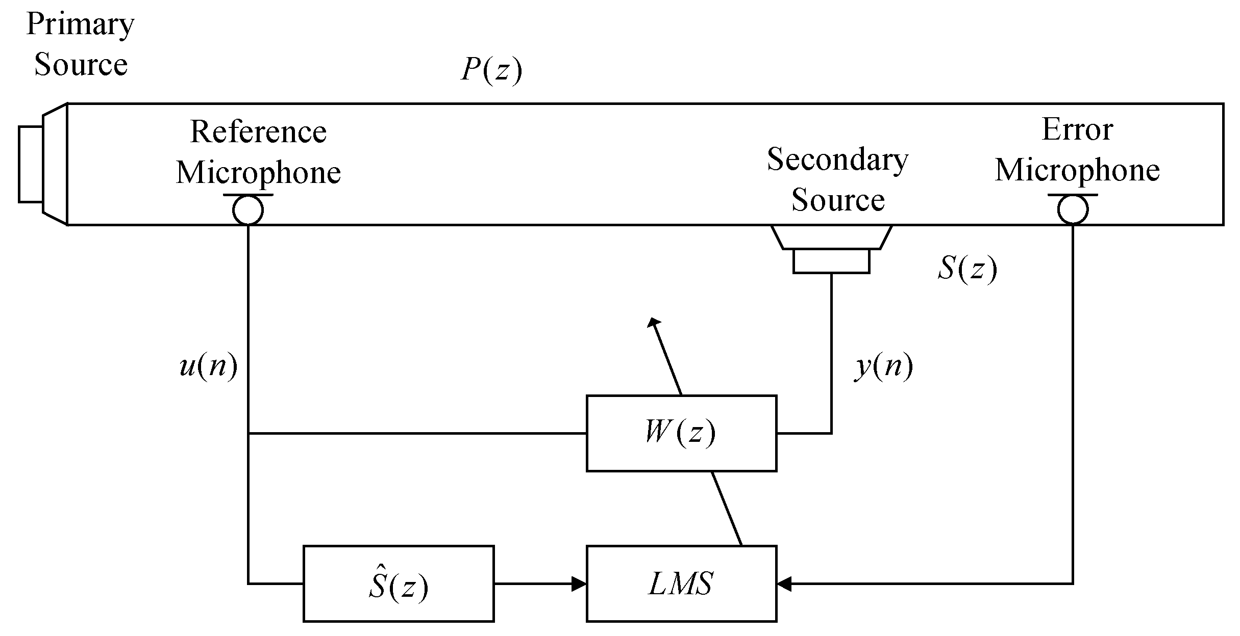
2.1. Linear Feedforward ANC System
2.2. Nonlinear Feedforward ANC System
3. Proposed Algorithm
3.1. DVMFXLMS
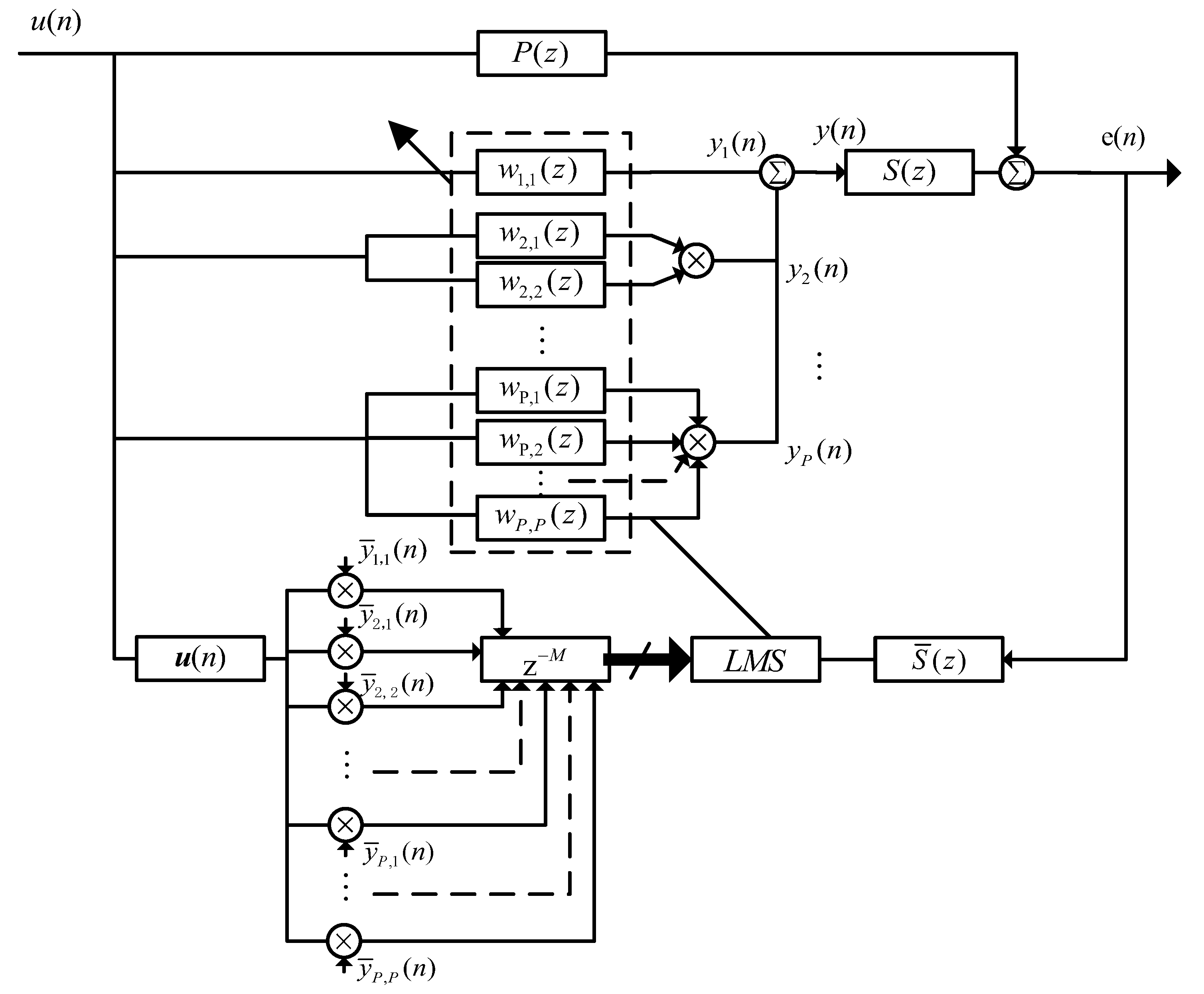
3.2. DVMFELMS
| Algorithm 1 Pseudo code of the proposed DVMFELMS algorithm. |
| Input:L, M, P, ,reference signals , desired signals , secondary path , adjoint virtual secondary path |
| Initialization: |
|
| Iteration: |
|
| Output: error signals , output signals , and filter coefficients |
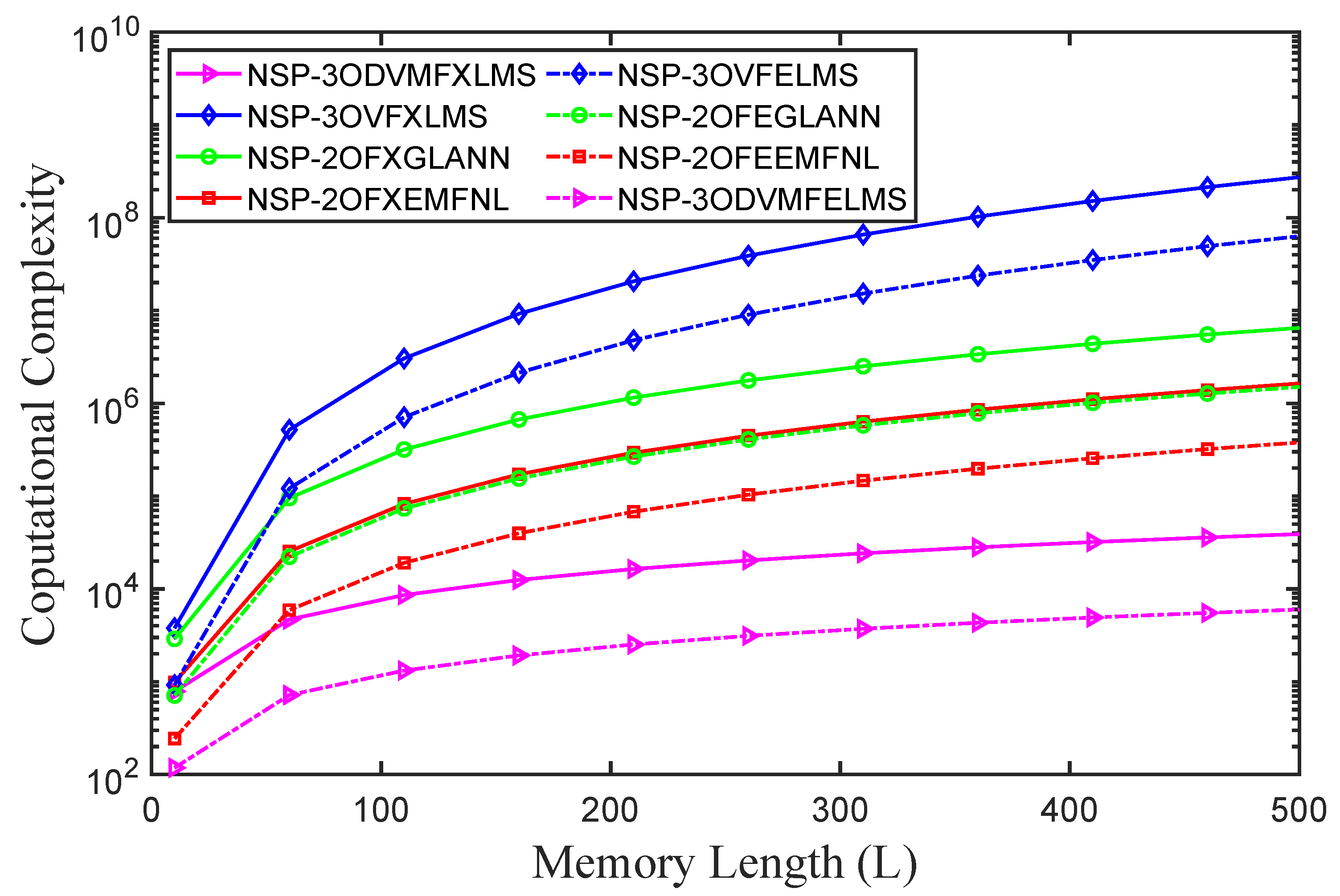
4. Computational Complexity
5. Performance Evaluation
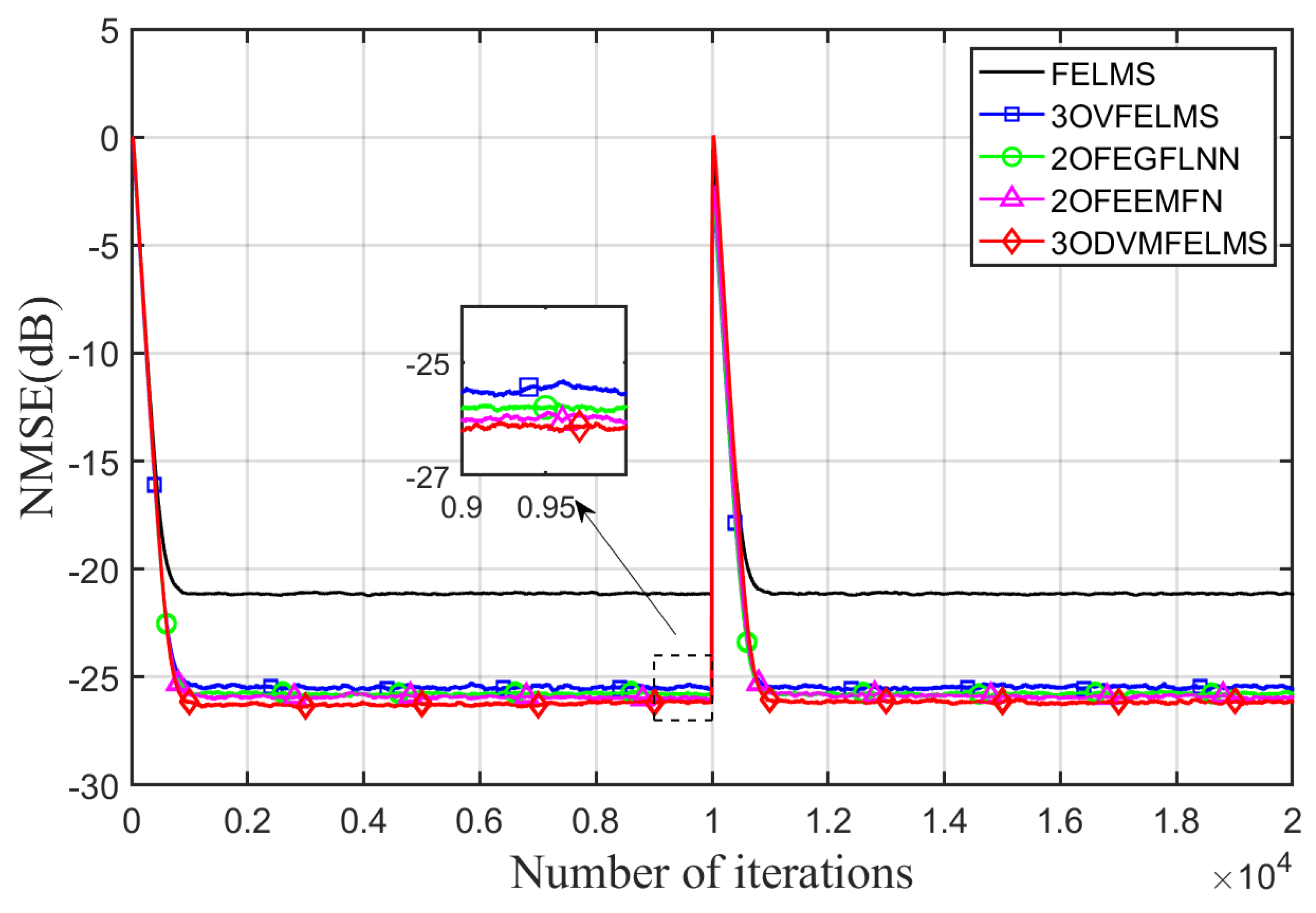
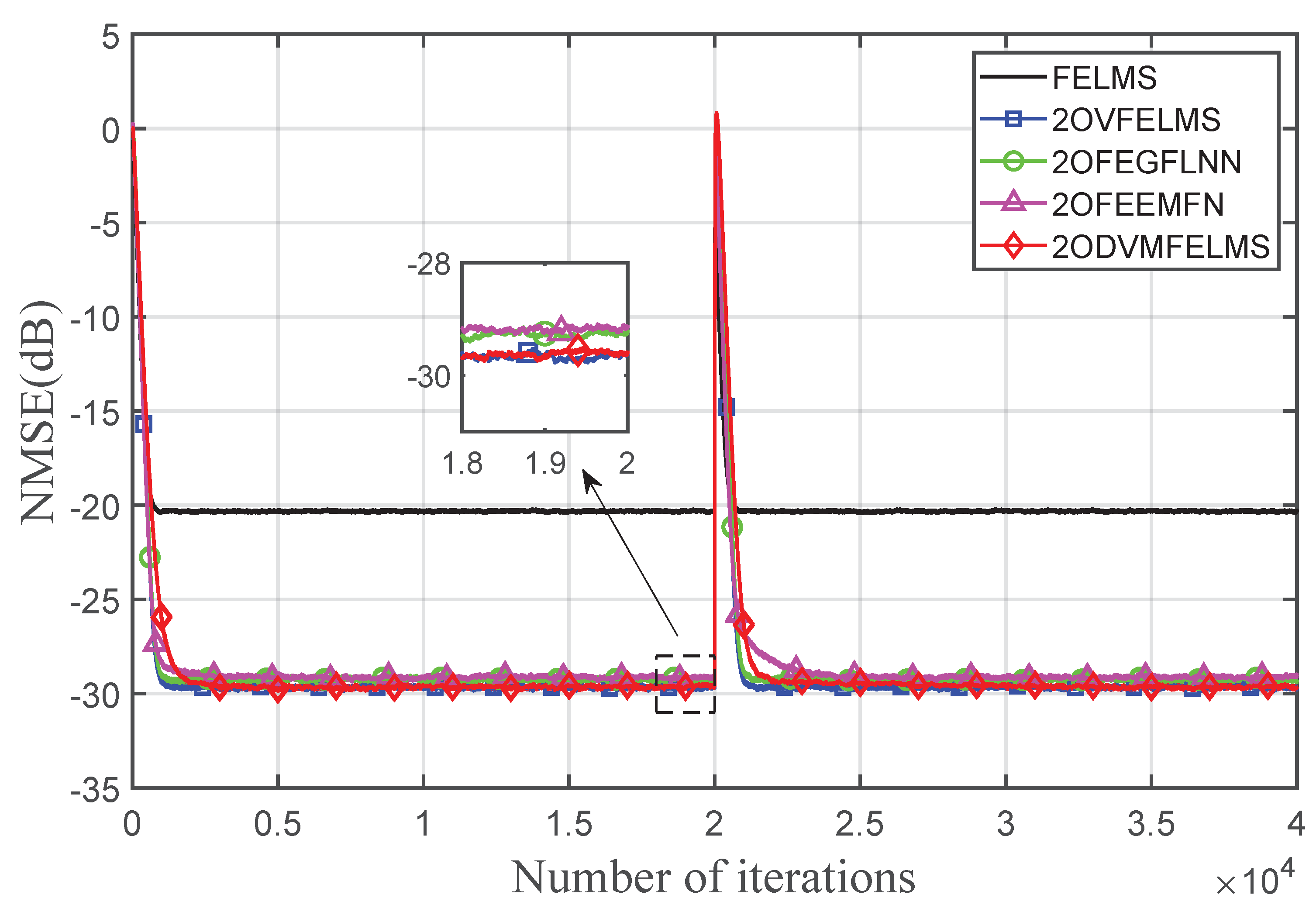
5.1. Simulation with Nonlinear Primary Path
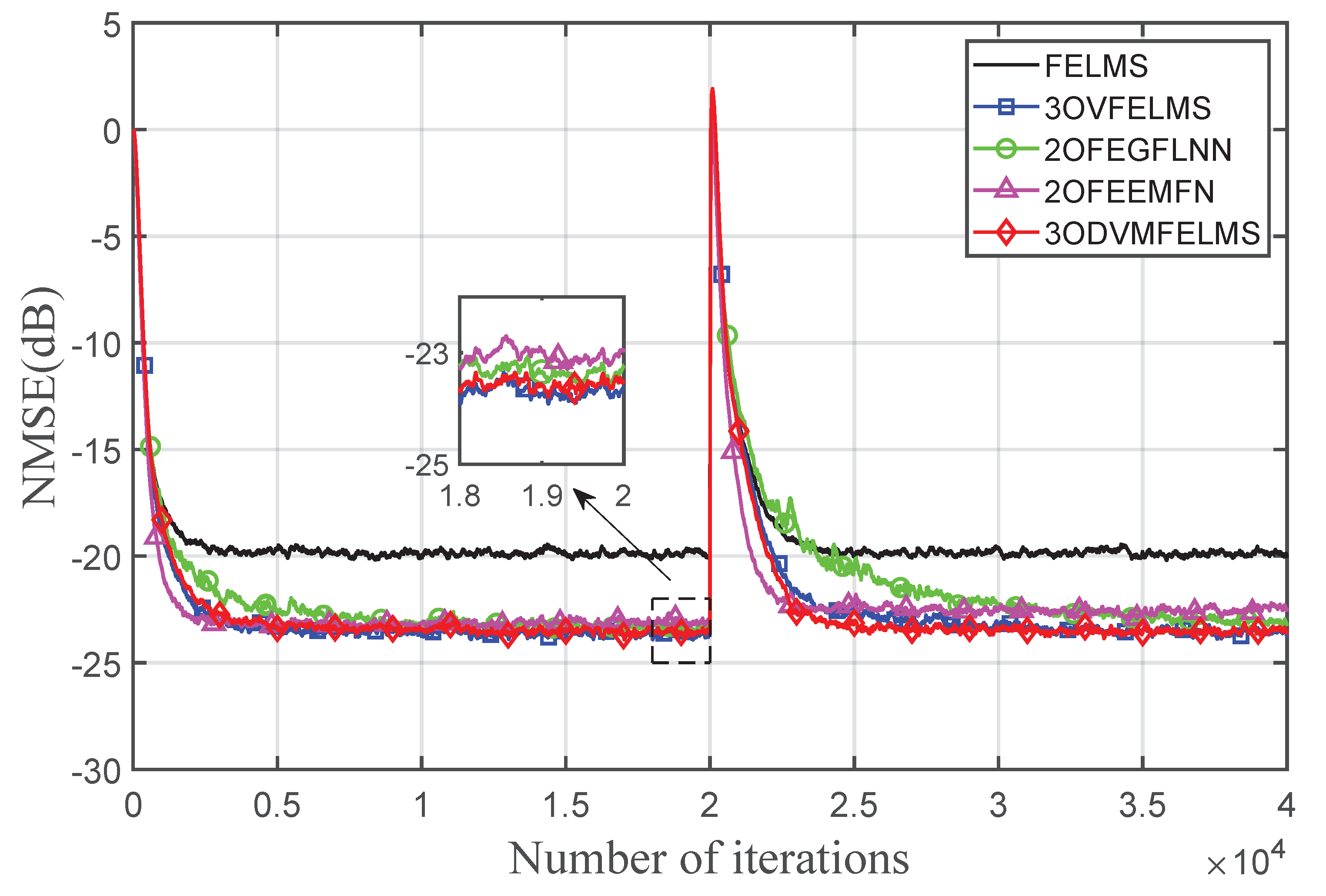
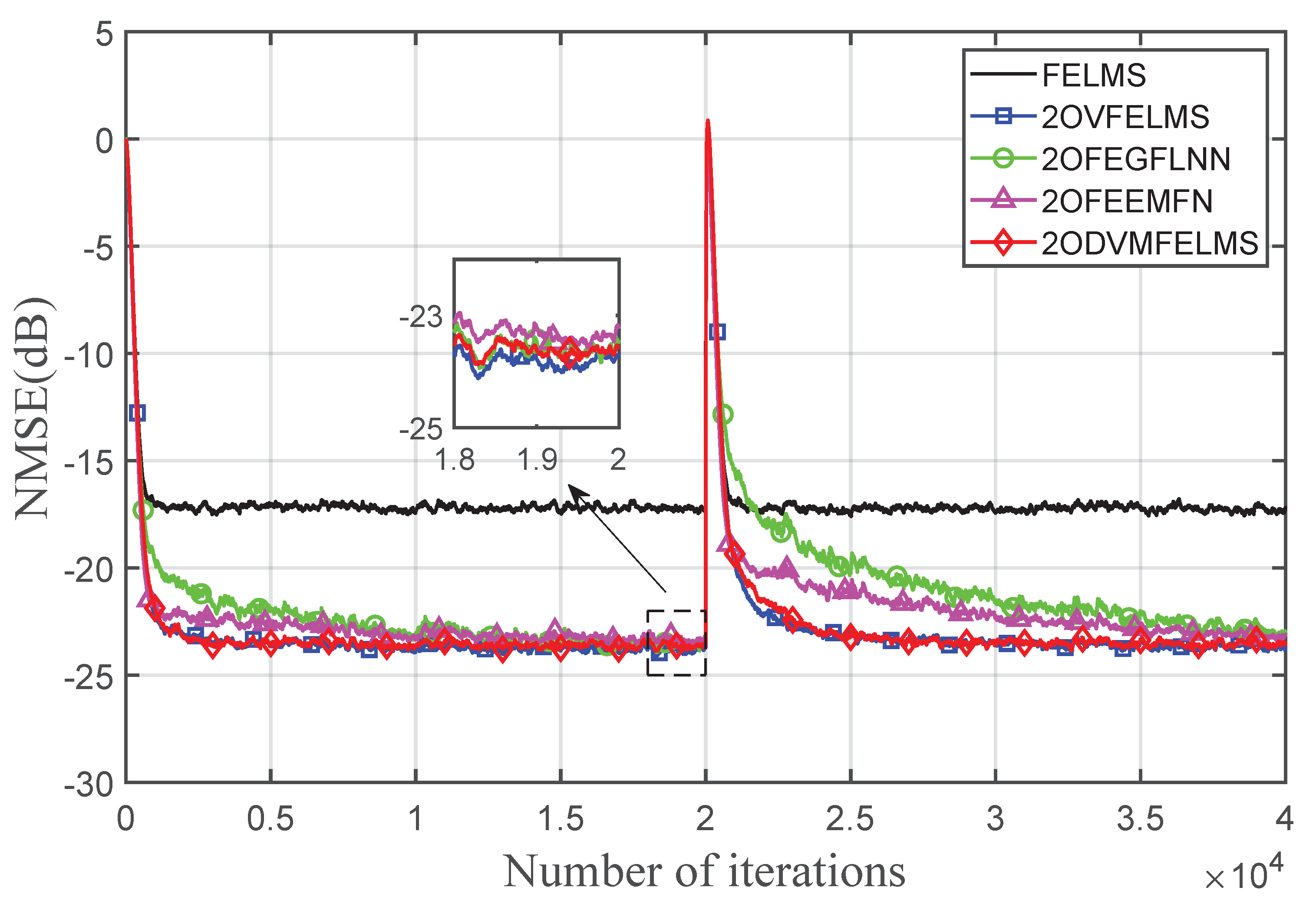
5.2. Simulation with Nonlinear Primary Path and Nonlinear Secondary Path
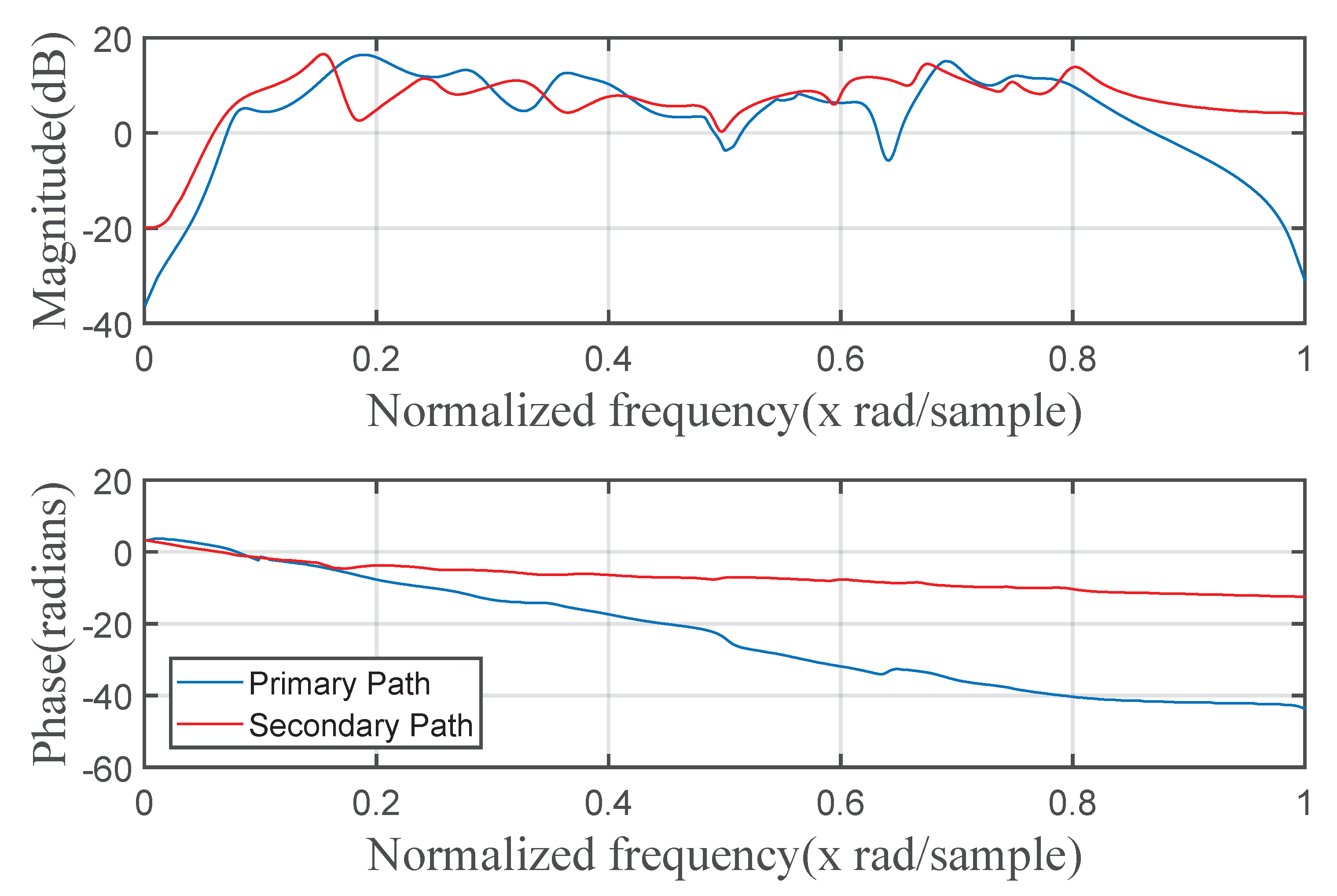
5.3. Simulation with Measured Primary Path and Secondary Path
6. Conclusions
Author Contributions
Funding
Institutional Review Board Statement
Informed Consent Statement
Data Availability Statement
Conflicts of Interest
Abbreviations
| FXLMS | Filtered-Reference Least Mean Square |
| FELMS | Filtered-Error Least Mean Square |
| FIR | Finite Impulse Response |
| IIR | Infinite Impulse Response |
| NANC | Nonlinear Active Noise Control |
| LSP | Linear Secondary Path |
| NSP | Nonlinear Secondary Path |
| FLNN | Functional Link Neural Network |
| GFLNN | Generalized Functional Link Neural Network |
| EFLNN | Exponential Functional Link Neural Network |
| EMFN | Even Mirror Fourier Nonlinear |
| LeNN | Legendre Neural Network |
| VFXLMS | Volterra Filtered-Reference Least Mean Square |
| VFELMS | Volterra Filtered-Error Least Mean Square |
| DVMFXLMS | Volterra Filtered-Reference Least Mean Square Based on Decomposable Volterra Model |
| DVMFELMS | Volterra Filtered-Error Least Mean Square Based on Decomposable Volterra Model |
| FXGFLNN | Filtered-Reference Functional Link Neural Network |
| FEGFLNN | Filtered-Error Functional Link Neural Network |
| FXEMFNL | Filtered-Reference Even Mirror Fourier Nonlinear Filter with a Linear Part |
| FEEMFNL | Filtered-Error Even Mirror Fourier Nonlinear Filter with a Linear Part |
| NMSE | Normalized Mean Square Error |
| SNR | Signal-to-Noise Ratio |
References
- Elliott, S.J. Signal Processing for Active Control; Academic: New York, NY, USA, 2001. [Google Scholar]
- Hansen, C.; Snyder, S.; Qiu, X.; Brooks, L.; Moreau, D. Active Control of Noise and Vibration; CRC Press: Boca Raton, FL, USA, 2012. [Google Scholar]
- Kuo, S.M.; Morgan, D.R. Active noise control: A tutorial review. Proc. IEEE 1999, 87, 943–973. [Google Scholar] [CrossRef] [Green Version]
- Cheer, J.; Elliott, S.J. Multichannel control systems for the attenuation of interior road noise in vehicles. Mech. Syst. Signal Process. 2015, 60–61, 753–769. [Google Scholar] [CrossRef] [Green Version]
- Kajikawa, Y.; Gan, W.S.; Kuo, S.M. Recent advances on active noise control: Open issues and innovative applications. APSIPA Trans. Signal Inf. Process. 2012, e3, 753–769. [Google Scholar] [CrossRef] [Green Version]
- Han, R.; Wu, M.; Gong, C.; Jia, S.; Han, T.; Sun, H.; Yang, J. Combination of robust algorithm and head-tracking for a feedforward active headrest. Appl. Sci. 2019, 9, 1760. [Google Scholar] [CrossRef] [Green Version]
- Rafaely, B. Zones of quiet in a broadband diffuse sound field. J. Acoust. Soc. Am. 2001, 110, 296–302. [Google Scholar] [CrossRef] [Green Version]
- Elliott, S.J.; Cheer, J. Modeling local active sound control with remote sensors in spatially random pressure fields. J. Acoust. Soc. Am. 2015, 137, 1936–1946. [Google Scholar] [CrossRef] [PubMed] [Green Version]
- Rafaely, B.; Elliott, S.J. A computationally efficient frequency-domain LMS algorithm with constraints on the adaptive filter. IEEE Trans. Signal Process. 2000, 48, 1649–1655. [Google Scholar] [CrossRef]
- Zhang, G.; Tao, J.; Qiu, X.; Burnett, I. Decentralized two-channel active noise control for single frequency by shaping matrix eigenvalues. IEEE/ACM Trans. Audio Speech Lang. Process. 2019, 27, 44–52. [Google Scholar] [CrossRef]
- Tan, L.; Jiang, J. Adaptive volterra filters for active control of nonlinear noise processes. IEEE Trans. Signal Process. 2001, 49, 1667–1676. [Google Scholar] [CrossRef]
- Zhu, L.; Yang, T.; Pan, J. Design of nonlinear active noise control earmuffs for excessively high noise level. J. Acoust. Soc. Am. 2019, 146, 1547–1555. [Google Scholar] [CrossRef] [PubMed]
- George, N.V.; Panda, G. Advances in active noise control: A survey, with emphasis on recent nonlinear techniques. Signal Process. 2013, 93, 363–377. [Google Scholar] [CrossRef]
- Lu, L.; Yin, K.L.; de Lamare, R.C.; Zheng, Z.; Yu, Y.; Yang, X.; Chen, B. A survey on active noise control in the past decade–part II: Nonlinear systems. Signal Process. 2020, 181, 10729. [Google Scholar]
- Snyder, S.D.; Tanaka, N. Active control of vibration using a neural network. IEEE Trans. Neural Netw. 1995, 6, 819–828. [Google Scholar] [CrossRef]
- Zhou, Y.L.; Zhang, Q.Z.; Li, X.D.; Gan, W.S. Analysis and DSP implementation of an ANC system using a filtered-error neural network. J. Sound Vib. 2005, 285, 1–25. [Google Scholar] [CrossRef]
- Sicuranza, G.L.; Carini, A. Filtered-x affine projection algorithm for multichannel active noise control using second-order volterra filters. IEEE Signal Process. Lett. 2004, 11, 853–857. [Google Scholar] [CrossRef]
- Das, D.P.; Panda, G. Active mitigation of nonlinear noise processes using a novel filtered-s LMS algorithm. IEEE/ACM Trans. Audio Speech Lang. Process. 2004, 12, 313–322. [Google Scholar] [CrossRef]
- Sicuranza, G.; Carini, A. A generalized FLANN filter for nonlinear active noise control. IEEE/ACM Trans. Audio Speech Lang. Process. 2011, 19, 2412–2417. [Google Scholar] [CrossRef]
- Patel, V.; Gandhi, V.; Heda, S.; George, N.V. Design of adaptive exponential functional link network-based nonlinear filters. IEEE Trans. Circuits Syst. I Reg. Pap. 2016, 63, 1434–1442. [Google Scholar] [CrossRef]
- Carini, A.; Sicuranza, G.L. Even mirror fourier nonlinear filters. In Proceedings of the 2013 IEEE International Conference on Acoustics, Speech and Signal Processing, Vancouver, BC, Canada, 26–31 May 2013; pp. 5608–5612. [Google Scholar]
- Carini, A.; Cecchi, S.; Romoli, L.; Sicuranza, G.L. Legendre nonlinear filters. Signal Process. 2015, 109, 84–94. [Google Scholar] [CrossRef]
- Carini, A.; Sicuranza, G.L. A study about chebyshev nonlinear filters. Signal Process. 2016, 122, 24–32. [Google Scholar] [CrossRef]
- Chen, B.; Yu, S.; Yu, Y.; Guo, R. Nonlinear active noise control system based on correlated EMD and chebyshev filter. Mech. Syst. Signal Process. 2019, 130, 74–86. [Google Scholar] [CrossRef]
- George, N.V.; Gonzalez, A. Convex combination of nonlinear adaptive filters for active noise control. Appl. Acoust. 2014, 76, 157–161. [Google Scholar] [CrossRef]
- Zhao, H.; Zeng, X.; He, Z.; Yu, S.; Chen, B. Improved functional link artificial neural network via convex combination for nonlinear active noise control. Appl. Soft Comput. 2016, 42, 351–359. [Google Scholar] [CrossRef] [Green Version]
- Zhou, D.; Debrunner, V. Efficient adaptive nonlinear filters for nonlinear active noise control. IEEE Trans. Circuits Syst. I Reg. Pap. 2007, 54, 669–681. [Google Scholar] [CrossRef]
- Kuo, S.M.; Wu, H.T. Nonlinear adaptive bilinear filters for active noise control systems. IEEE Trans. Circuits Syst. I Reg. Pap. 2005, 52, 617–624. [Google Scholar] [CrossRef]
- Tan, L.; Dong, C.; Du, S. On implementation of adaptive bilinear filters for nonlinear active noise control. Appl. Acoust. 2016, 106, 122–128. [Google Scholar] [CrossRef]
- Zhao, H.; Zeng, X.; He, Z.; Li, T. Adaptive RSOV filter using the felms algorithm for nonlinear active noise control systems. Mech. Syst. Signal Process. 2013, 34, 378–392. [Google Scholar] [CrossRef]
- Carini, A.; Sicuranza, G.L. Recursive even mirror fourier nonlinear filters and simplified structures. IEEE Trans. Signal Process. 2014, 62, 6534–6544. [Google Scholar] [CrossRef]
- Guo, X.; Jiang, J.; Tan, L.; Du, S. Improved adaptive recursive even mirror fourier nonlinear filter for nonlinear active noise control. Appl. Acoust. 2018, 146, 310–319. [Google Scholar] [CrossRef]
- Le, D.C.; Zhang, J.; Pang, Y. A bilinear functional link artificial neural network filter for nonlinear active noise control and its stability condition. Appl. Acoust. 2018, 132, 19–25. [Google Scholar] [CrossRef]
- Guo, X.; Jiang, J.; Chen, J.; Du, S.; Tan, L. Bibo-stable implementation of adaptive function expansion bilinear filter for nonlinear active noise control. Appl. Acoust. 2020, 168, 107407. [Google Scholar] [CrossRef]
- Carini, A.; Sicuranza, G.L. Bibo-stable recursive functional link polynomial filters. IEEE Trans. Signal Process. 2017, 65, 1595–1606. [Google Scholar] [CrossRef]
- Fermo, A.; Carini, A.; Sicuranza, G.L. Low-complexity nonlinear adaptive filters for acoustic echo cancellation in GSM handset receivers. Eur. Trans. Telecommun. 2003, 14, 161–169. [Google Scholar] [CrossRef]
- Paleologu, C.; Benesty, J.; Ciochină, S. Linear system identification based on a kronecker product decomposition. IEEE/ACM Trans. Audio Speech Lang. Process. 2018, 26, 1793–1808. [Google Scholar] [CrossRef]
- Pinheiro, F.C.; Lopes, C.G. A low-complexity nonlinear least mean squares filter based on a decomposable volterra model. IEEE Trans. Signal Process. 2019, 67, 5463–5478. [Google Scholar] [CrossRef]
- Guo, X.; Li, Y.; Jiang, J.; Dong, C.; Du, S.; Tan, L. Sparse modeling of nonlinear secondary path for nonlinear active noise control. IEEE Trans. Instrum. Meas. 2018, 67, 482–496. [Google Scholar] [CrossRef]
- Miyagi, S.; Sakai, H. Performance comparison between the filtered-error LMS and the filtered-x LMS algorithms ANC. In Proceedings of the 2001 IEEE International Symposium on Circuits and Systems, Sydney, NSW, Australia, 6–9 May 2001; pp. 661–664. [Google Scholar]


| Algorithm | VFXLMS | FXGFLNN | 2OFXEMFNL | DVMFXLMS |
|---|---|---|---|---|
| Inputs signal | 1 | |||
| Output signal | P | |||
| Filtered signal | ||||
| Weight update | ||||
| Total |
| Algorithm | VFELMS | FEGFLNN | 2OFEEMFNL | DVMFELMS |
|---|---|---|---|---|
| Inputs signal | 1 | |||
| Output signal | P | |||
| Filtered signal | M | M | M | M |
| Weight update | ||||
| Total |
Publisher’s Note: MDPI stays neutral with regard to jurisdictional claims in published maps and institutional affiliations. |
© 2021 by the authors. Licensee MDPI, Basel, Switzerland. This article is an open access article distributed under the terms and conditions of the Creative Commons Attribution (CC BY) license (https://creativecommons.org/licenses/by/4.0/).
Share and Cite
Zhang, J.; Zheng, C.; Zhang, F.; Li, X. A Low-Complexity Volterra Filtered-Error LMS Algorithm with a Kronecker Product Decomposition. Appl. Sci. 2021, 11, 9637. https://doi.org/10.3390/app11209637
Zhang J, Zheng C, Zhang F, Li X. A Low-Complexity Volterra Filtered-Error LMS Algorithm with a Kronecker Product Decomposition. Applied Sciences. 2021; 11(20):9637. https://doi.org/10.3390/app11209637
Chicago/Turabian StyleZhang, Jinhui, Chengshi Zheng, Fangjie Zhang, and Xiaodong Li. 2021. "A Low-Complexity Volterra Filtered-Error LMS Algorithm with a Kronecker Product Decomposition" Applied Sciences 11, no. 20: 9637. https://doi.org/10.3390/app11209637
APA StyleZhang, J., Zheng, C., Zhang, F., & Li, X. (2021). A Low-Complexity Volterra Filtered-Error LMS Algorithm with a Kronecker Product Decomposition. Applied Sciences, 11(20), 9637. https://doi.org/10.3390/app11209637