Concept Drift Adaptation with Incremental–Decremental SVM

Abstract

Data classification in streams where the underlying distribution changes over time is known to be difficult. This problem—known as concept drift detection—involves two aspects: (i) detecting the concept drift and (ii) adapting the classifier. Online training only considers the most recent samples; they form the so-called shifting window. Dynamic adaptation to concept drift is performed by varying the width of the window. Defining an online Support Vector Machine (SVM) classifier able to cope with concept drift by dynamically changing the window size and avoiding retraining from scratch is currently an open problem. We introduce the Adaptive Incremental–Decremental SVM (AIDSVM), a model that adjusts the shifting window width using the Hoeffding statistical test. We evaluate AIDSVM performance on both synthetic and real-world drift datasets. Experiments show a significant accuracy improvement when encountering concept drift, compared with similar drift detection models defined in the literature. The AIDSVM is efficient, since it is not retrained from scratch after the shifting window slides.

1. Introduction

An important class of Machine Learning (ML) problems involves dealing with data that have to be classified on arrival. Usually, in these situations, historical data become less relevant for the ML task. Climate change forecasting is such an example. In the past, elaborate models have predicted how carbon emissions impact the warming of the environment quite well. However, given accelerated emission rates, the trends determined from past data have changed [1]. Typically, for these problems, the underlying distribution changes in time. There are many ML models that can approximate a stationary distribution when the number of samples increases to infinity [2]. A classifier that considers its entire history cannot be employed, since it will have poor generalization results, not to mention the technical difficulties raised by keeping all data. This pattern of evolution—for which intrinsic distribution of the data is not stationary—is called concept drift. As data evolve, it may be because of either noise or change; the distinction between them is made via persistence [3]. The concept drift models must combine robustness to noise or outliers with sensitivity to the concept drift [2].

Methods for coping with concept drift are presented in several comprehensive overviews [4,5,6]. An important topic is the embedding of drift detection into the learning algorithm. According to Farid et al. [7], there are three main approaches: instance-based (window-based), weight-based, and ensemble of classifiers. Window-based approaches usually adjust the window size considering the classification accuracy rate, while weight-based approaches discard past samples according to a computed importance. More recent studies [8,9] divide stream mining in the presence of concept drift into active (trigger-based) and passive (evolving) approaches. The active approaches update the model whenever a concept drift is detected, whereas the passive ones learn continuously, regardless of the drift. It is not sufficient to detect the concept drift; one would have to adapt the current model to the observed drift [6]. Some approaches retrain from scratch; they use distance-based classifiers, such as k-NNs or decision trees, for which they define removal strategies. Other approaches use an ensemble of models and discard the obsolete ones. Most of the works only report the overall accuracy. However, at the drift point, the performance of a model retrained from scratch drops, and it is followed by a slow recovery. This aspect is seldom presented, even if recovery after drift is important, as discussed by Raab et al. [10].

SVM is known to be one of the most reliable ML models for non-linearly separable input spaces. In current research trends, there are applications that inherently operate under concept drift. An SVM has been applied recently in news classification [11]. Soil temperatures were predicted by the use of a hybrid SVM whose parameters were tuned via firefly optimization [12]. This problem presents inherent seasonality in both input features and predicted outcome. A similar problem is that of land cover classification, approached most recently in [13]. This study is based on satellite imagery; the main source of data is the multi-temporal data acquired by the Sentinel-2 satellite. Drift is inherently present in this data, due to their temporal nature. Another study that employs SVM classification is one predicting COVID-19 incidence into three risk categories, based on features such as number of deaths, mobility, bed occupancy or number of patients in the ICU [14]. As health systems and the population adapts over time, these features may inherently be exposed to concept drift. The study concludes that between the ConvLSTM and SVM, the former performed better; this is not surprising, because a classic SVM is not designed for concept drift. An SVM is also used in hybrid approaches in regression problems, such as predicting the lead time needed for shipyards to arrange production plans [15], or modelling pan evaporation [16], phenomena that could also present drift, given their temporal nature.

Some SVM models were especially adapted for concept drift handling [17,18,19]. However, adapting the window to the concept drift requires classifier retraining on the new window, which is computationally inefficient. The SVM models in [17,18,19] do not consider the presence of concept drift and assume stationary conditions for the input data. Defining an online SVM classifier able to cope with concept drift by dynamically changing the window size and avoiding retraining from scratch is currently an open problem. We believe that, considering the drift, the accuracy obtained by the SVM model has the potential to improve.

The ability of the incremental–decremental SVM model to naturally adapt to concept drift, combined with the power of the Hoeffding test (Hoeffding inequality theorem [20]) used for determining the obsolescence of past samples, gave us the raw inspiration for our work.

Our contribution is the introduction of the Adaptive Incremental–Decremental SVM (AIDSVM) algorithm, a generalization of the incremental–decremental SVM, capable of dynamically detecting the concept drift and adjusting the width of the shifting window accordingly. To our knowledge, our model is the first incremental SVM classifier using dynamic adaptation of the shifting window. According to our experiments, it has the same or better accuracy compared with common drift-aware classifiers on some of the most common synthetic and real-world datasets. Experimental evidence shows that AIDSVM-detected drift positions are close to the theoretical drift points. We provide the source code of our algorithm on Github as a Python implementation (https://github.com/hash2100/aidsvm, accessed on 2 October 2021).

The rest of the article is structured as follows. We present related work and the state of the art in concept drift with adaptive windows in Section 2. To make the paper self-contained, Section 3 summarizes notations and previous results we use in our approach: the ADWIN principle of detecting concept drift based on the Hoeffding bound and the incremental–decremental SVM. Section 4 introduces the AIDSVM algorithm. Experimental results on synthetic and real datasets are described in Section 5, where we compare our method with current approaches in concept drift. Section 6 summarizes the main achievements of our work and discusses further possible extensions.

2. Related Work: Concept Drift with Adaptive Shifting Windows

In this section, we list some of the most recent concept drift models based on adaptive windows, with a focus on SVM approaches.

Several models addressing concept drift on adaptive windows were proposed in recent years. Detailed overviews are given by the work of Iwashita et al. [5], Lu et al. [6], as well as Gemaque et al. [21]. The Learn++.NSE algorithm [22,23] and its fast version  [24] generate a new classifier for each received batch of data, and add the classifier to an existing ensemble. The classifiers are later combined using dynamically weighted majority voting, based on the classifier’s age. In [25], the adaptive random forest algorithm, used for the classification of evolving data streams, combines batch algorithm traits with dynamic update methods.

One of the seminal papers in this field is the Drift Detection Method (DDM) described in [26]. It uses the classification error as evidence of concept drift. The classification error decreases as the model learns the newer samples. The model establishes a warning level and a drift level. When the classification error increases over the warning level, newer samples are introduced into a special window. Once the error increases over the drift level, a new model is created, starting from the samples from the special window. A later extension, the Early Drift Detection Method (EDDM) [27], uses the distance between two consecutive errors and its standard deviation instead of the simple error rate used in the DDM. It also follows the same principle of comparing the error rate against warning and drift thresholds. Both methods are designed to operate regardless of the incremental learner used.

The Fast Hoeffding Drift Detection Method (FHDDM) [28] detects the drift point using a constant-size sliding window. It detects a drift if a significant variation is observed between the current and the maximum accuracy. The accuracy difference threshold is determined using Hoeffding’s inequality theorem:

$$\begin{array}{c}\hfill Pr\left(\right|\overline{X}-E\left[\overline{X}\right|\ge {ϵ}_H])\le \delta ,\mathrm{where}{ϵ}_H=\sqrt{\frac{1}{2n}ln\frac{2}{\delta }}\end{array}$$

The FHDDM method is extended by maintaining windows of different sizes in the Stacked Fast Hoeffding Drift Detection Method (FHDDMS) [29]. This is employed to reduce detection delays. Extensive treatment of these two methods is shown in [30,31].

A very recent approach using the error rate is the Accurate Concept Drift Detection Method (ACDDM) [32]. The author analyzes the consistency of prequential error rate using Hoeffding’s inequality. At each step, the difference between the current error rate and the minimum error date is determined. This is compared against the threshold given by the Hoeffding inequality for a desired confidence level. The drift is detected when the error rate difference is greater than the computed deviation:

$$\begin{array}{c}\hfill ϵ\le \sqrt{\frac{1}{2n}ln\frac{1}{\delta }}\end{array}$$

The ACDDM is evaluated using the Very Fast Decision Tree learning algorithm ([32], Section 3).

Recently, SVMs were also used to address concept drift. ZareMoodi et al. [33] proposed an SVM classification model with a learned label space that evolves in time, where novel classes may emerge or old classes may disappear. For the modelling of intricate-shape class boundaries, they used support-vector-based data description methods. Yalcin et al. [34] used SVMs in an ensemble-based incremental learning algorithm to model the changing environments. Learning windows of variable length also appear in the papers of Klinkenberg et al. [17] and Klinkenberg [18]. Klinkenberg’s methods use a variable width window, which is adjusted by the estimation of classification generalization error. At each time step, the algorithm builds several SVM models with various window sizes, then it selects the one that minimizes the error estimate. The appropriate window size is automatically computed, and so is the selection of samples and their weights. While the methods used by Klinkenberg et al. can be used online in applications, they are not incremental and the SVMs must be retrained. Another approach proposes an adaptive dynamic ensemble of SVMs which are trained on multiple subsets of the initial dataset [19]. The most recent heuristic approach splits the stream into data blocks of the same size, and uses the next block to assess the performance of the model trained on the current block [35].

3. Background: The Adaptive Window Model for Drift Detection and the Incremental–Decremental SVM

To make the paper self-contained, we summarize in the following two techniques incorporated in the AIDSVM method: the statistical test used for concept drift detection, and the incremental–decremental SVM procedure used to discard the obsolete part of the window.

3.1. Concept Drift with Adaptive Window

We use the ADWIN adapting window strategy to cope with concept drift. Details can be found in the original paper [20].

During learning, past data, up to the current sample, are stored in a fixed-size window. For every sample $x_i$ in the window characterized by its class $y_i$, the trained model predicts class $\widehat{y_i}$; we compute the sample error $e_i$ which is 0 if $y_i=\widehat{y_i}$ or 1 if the predicted label is wrong. Given a set of samples, the prediction error $e_i$ is a random variable that follows a Bernoulli distribution. The sum of these errors, for a set of samples, is a random variable following a binomial distribution. If the width of the window is n, where $x_i$ ($i=1,\cdots ,n$) are the window samples, then the model error rate is the probability $p_i$ of observing 1 in the sequence of $e_j$ errors ($j=1,\cdots ,i$). Each $p_i$ is drawn from a distribution $D_i$. In the ideal case of no concept drift, all $D_i$ distributions are identical. With concept drift, the distribution changes, as the error rate is expected to increase.

The ADWIN strategy successively splits the current window of n elements into two “large enough” sub-windows. If these sub-windows show “different enough” averages of their sample error, then the expected values corresponding to the two binomial distributions are different. By incrementing the i value, the approach constructs all possible cuts of the current window into two adjacent splits ($W_0$, $W_1$), where $W_0$ has $n_0$ samples $x_1,x_2,\cdots ,x_i$ and $W_1$ has $n_1$ samples $x_{i+1},\cdots ,x_n$. We have $n=n_0+n_1$. As cuts are constructed, they are evaluated against the following Hoeffding test:

$$Pr\left(\right|{\mu }_0-{\mu }_1|\ge {ϵ}_{cut})\le \frac{\delta }{n}$$

(1)

where ${\mu }_0$ and ${\mu }_1$ are the averages for the error values in $W_0$ and $W_1$, and $\delta \in (0,1)$ is the required global error. The scaling $\frac{\delta }{n}$ is required by the Bonferroni correction, since we perform multiple hypothesis testing by repeatedly splitting the samples. The statistical test checks whether the observed averages differ by more than a threshold ${ϵ}_{cut}$, which is dependent on the window split size.

The null hypothesis $H_0$ assumes that the mean $\mu$ has remained constant along all the sufficient “large enough” cuts performed on the sliding window W. Parameter $\delta$ tunes the test’s confidence; for example, a 95% confidence level is assimilated to $\delta =0.05$. The statistical test for observing different distributions in $W_0$ and $W_1$ checks whether the observed averages in both sub-windows differ by more than the threshold ${ϵ}_{cut}$. Given a specified confidence parameter $\delta$, it was shown in [20] that the maximum acceptable difference ${ϵ}_{cut}$ is:

$${ϵ}_{cut}=\sqrt{\frac{1}{2m}·ln\frac{4}{{\delta }^{\prime }}}$$

(2)

where:

$$\begin{array}{cc}\hfill m=\frac{1}{1/n_0+1/n_1}(\mathrm{the}\mathrm{harmonic}\mathrm{mean}\mathrm{of}{n}_0\mathrm{and}{n}_1),& {\delta }^{\prime }=\frac{\delta }{n}\end{array}$$

(3)

However, this approach is too conservative. Based on the Hoeffding bound, it overestimates the probability of large deviations for small variance distributions, assuming the variance is ${\sigma }^2=0.25$, which is the worst-case scenario. A more appropriate test used in [20] also takes the window variance into consideration:

$$\begin{array}{c}\hfill {ϵ}_{cut\_adjusted}=\sqrt{\frac{2}{m}·{\sigma }_W^2·ln\frac{2}{{\delta }^{\prime }}}+\frac{2}{3m}ln\frac{2}{{\delta }^{\prime }}\end{array}$$

(4)

In Equation (4), the square root term actually adjusts the ${ϵ}_{cut}$ term relative to the standard deviation, whereas the additional term guards against the cases where the window sizes are too small.

An exemplification of these criteria is given in Figure 1. We considered a window of 1000 simulated samples. For all samples $x_i$ inside the sliding window, we constructed the error $e_i$ using several simulated Bernoulli distributions. Afterwards, we computed the average error difference for each window split. A reference classifier with 85% accuracy, with no drift, is simulated with a Bernoulli distribution of p = 0.15. We simulated 20 such distributions. For drift simulation, we created 20 mixed distributions by concatenating the first 700 samples from a Bernoulli distribution with p = 0.15, with the last 300 samples from another Bernoulli distribution with p = 0.4. Thus, we simulated a sudden drop in the classifier’s accuracy from 85% to 60%. Then, we obtained the test margins ${ϵ}_{cut}$ and ${ϵ}_{cut\_adjusted}$ from Equations (2) and (4) by successive splits of $W_0$ and $W_1$ for the shifting window, imposing a limit of at least 41 samples (for statistical relevance). In Figure 1, it can be seen that the two margins, ${ϵ}_{cut}$ and ${ϵ}_{cut\_adjusted}$, are somewhat similar. However, the adjusted threshold (${ϵ}_{cut\_adjusted}$) is more resilient to false positives on smaller partitions, and more conservative on larger ones.

3.2. Kuhn–Tucker Conditions and Vector Migration in Incremental–Decremental SVMs

Among the SVM models suitable for adapting to drifting environments, the incremental SVM learning algorithm of Cauwenberghs and Poggio [36] (later extended in [37]) is well equipped for handling non-linearly separable input spaces. By design, it is also able to non-destructively forget samples, adapting its statistical model to the remaining data samples. Retraining from scratch is thus avoided, and the model can learn/unlearn much faster than a traditional SVM. An efficient implementation for individual learning of the CP algorithm was analyzed by Laskov [38], along with a similar algorithm for one-class learning. Practical implementation issues of the CP algorithm were discussed in [39,40]. The algorithm was also adapted for regression [41,42,43]. The incremental approach was revisited more recently in [44], where a linear exponential cost-sensitive incremental SVM was defined. In the following, Equations (5)–(14) are taken from [39]. Our AIDSVM method is based on the CP algorithm. Therefore, we briefly review the theoretical framework, with emphasis on the Kuhn–Tucker conditions and exact vector migration relations, which were previously presented in [39] with full details.

For a set of samples $x_i$ with associated labels $y_i\in \{-1,+1\}$ ($i=1,\cdots ,N$), a linear SVM computes the separation hyperplane as a linear combination of the input samples given by the function $g\left(x\right)=w^{T}x+b$, where the predicted label is given by ${\widehat{y}}_i=sign\left(g\left(x_i\right)\right)$.

The optimal hyperplane is determined by the following optimization problem:

$$\begin{array}{cc}\hfill & \underset{w}{min}\frac{1}{2}{\parallel w\parallel }^2+C\sum _{i=1}^N{\xi }_i\hfill \end{array}$$

(5)

$$\begin{array}{cc}\hfill & \mathrm{subject}\mathrm{to}{y}_i(w^T{x}_i+b)\ge 1-{\xi }_i,{\xi }_i\ge 0,i=1,\cdots ,N\hfill \end{array}$$

(6)

where C is the regularization constant tuning the constraints strength. We define the penalty function $h\left(x_i\right)$ for data samples $x_i$ as:

$$\begin{array}{c}\hfill h\left(x_i\right)=y_{i}g\left(x_i\right)-1=y_i(w^T{x}_i+b)-1\end{array}$$

(7)

If $x_i$ is correctly classified, $h\left(x_i\right)$ would be positive; the variable associated with the constraint, ${\xi }_i$, is zero in this case. Otherwise, if incorrectly classified, or on the right side of the hyperplane, but at a smaller distance than the minimum margin $\frac{1}{2}\parallel w\parallel$, the value $h\left(x_i\right)$ becomes negative.

If sample $x_i$ is not classified correctly within a sufficient margin distance, $h\left(x_i\right)<0$ and ${\xi }_i>0$. However, Equation (5) enforces small ${\xi }_i$ penalties. The C regularization parameter tunes the trade-off between margin increase and correct classification.

Solving the constraint optimization problem makes use of the Kuhn–Tucker (KT) conditions; two of them are relevant for the incremental–decremental approach:

$$\begin{array}{ccc}\hfill & {\lambda }_i[h\left(x_i\right)+{\xi }_i]=0\hfill & \hfill i=1,\cdots ,N\end{array}$$

(8)

$$\begin{array}{ccc}\hfill & h\left(x_i\right)+{\xi }_i\ge 0\hfill & \hfill i=1,\cdots ,N\end{array}$$

(9)

Applying the KT conditions also determines the separation hyperplane to be computed as $g\left(x_i\right)={\sum }_{j=1}^N{\lambda }_j{y}_j{x}_j^T{x}_i+b$. Condition (8) is the complementary slackness condition. If ${\lambda }_i=0$, then the vector is not part of the solution at all. If non-zero, then (9) must be true, and $x_i$ will be part of the solution. When ${\xi }_i=0$ and $h\left(x_i\right)=0$, sample $x_i$ will be considered a support vector.

The penalty $h\left(x_i\right)$ can be:

$$\begin{array}{c}\hfill h\left(x_i\right)\left\{\begin{array}{cc}>0,\hfill & {\lambda }_i=0\mathrm{and}{\xi }_i=0\hfill \\ =0,\hfill & 0<{\lambda }_i<C,\hfill \\ \hfill & h\left(x_i\right)+{\xi }_i=0\mathrm{with}{\xi }_i=0\hfill \\ <0,\hfill & {\lambda }_i=C,\hfill \\ \hfill & h\left(x_i\right)+{\xi }_i=0\mathrm{with}{\xi }_i>0\hfill \end{array}\right.\end{array}$$

(10)

Based on these conditions, a vector $x_i$ could belong to one of the following sets: (i) support vectors, where $h\left(x_i\right)=0$ and $0<{\lambda }_i<C$, defining the hyperplane, (ii) error vectors, where $h\left(x_i\right)<0$ and ${\lambda }_i=C$, vectors situated on the wrong side of the separation hyperplane (or in the separation region), and (iii) rest vectors, where $h\left(x_i\right)>0$ and ${\lambda }_i=0$, vectors situated on the correct side of the separation hyperplane.

We map the input to a multi-dimensional space characterized by a kernel $K(·,·)$ and use the notation:

$$\begin{array}{c}\hfill Q_{ij}=y_i{y}_{j}K(x_i,x_j)\end{array}$$

(11)

We generalize the penalty function to $h\left(x_i\right)={\sum }_j{\lambda }_j{Q}_{ij}+b{y}_i-1$.

Incremental–decremental training comes down to varying the ${\lambda }_i$ parameters so that the KT conditions are always fulfilled. These variations determine vector migrations between the previously mentioned sets of vectors. The variations are defined by:

$$\begin{array}{cc}\hfill & \left[\begin{array}{c}\Delta b\\ \Delta {\lambda }_s\end{array}\right]=\underset{{\beta }_s}{\underbrace{-{\left[\begin{array}{cc}0& y_s\\ y_s& Q_{ss}\end{array}\right]}^{-1}\left[\begin{array}{c}{y}_c\\ Q_{sc}\end{array}\right]}}\Delta {\lambda }_c\hfill \end{array}$$

(12)

$$\begin{array}{cc}\hfill & \left[\begin{array}{c}\Delta h_r\\ \Delta h_c\end{array}\right]=\underset{{\gamma }_s}{\underbrace{\left\{\left[\begin{array}{cc}{y}_r& Q_{rs}\\ y_c& Q_{cs}\end{array}\right]{\beta }_s+\left[\begin{array}{c}{Q}_{rc}\\ Q_{cc}\end{array}\right]\right\}}}\Delta {\lambda }_c\hfill \end{array}$$

(13)

where the ‘s’ index stands for support and the ‘r’ is used for both error or rest vector sets. By computing the exact increments of $\Delta {\lambda }_s$, we carefully trace vectors’ migrations among the sets, thus performing the learning/unlearning (which are symmetrical procedures). Considering the first relation, $\Delta {\lambda }_s={\beta }_s\Delta {\lambda }_c$, where ${\beta }_s$ is the s-th component of vector $\beta$, we find that $-{\lambda }_s\le \Delta {\lambda }_s\le C-{\lambda }_s$, and further that $-{\lambda }_s\le {\beta }_s\Delta {\lambda }_c\le C-{\lambda }_s$; this means, for the incremental case, that:

$$\begin{array}{c}\hfill \Delta {\lambda }_c=min\left\{\frac{C-{\lambda }_s}{{\beta }_s},-\frac{{\lambda }_s}{{\beta }_s}\right\}\end{array}$$

(14)

Equation (14) is for support vectors only; a similar equation can be written for the rest vectors. The entire discussion has already been provided in detail in [39].

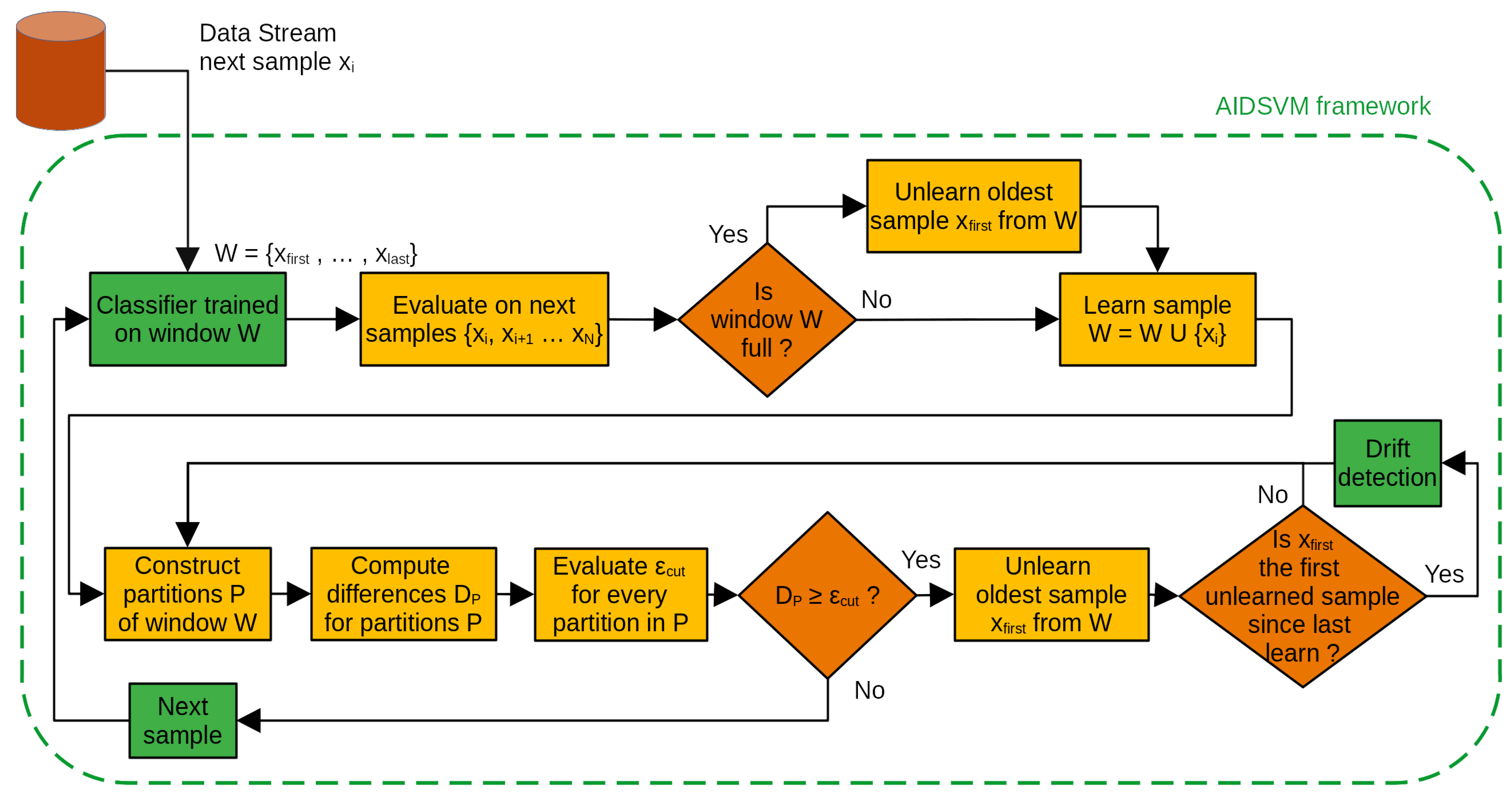
4. Adaptive-Window Incremental–Decremental SVM (AIDSVM)

We are now ready to introduce the AIDSVM algorithm, which is a generalization of the CP algorithm for concept drift, using an adaptive shifting window.

Using the classification terminology [7,8,9], AIDSVM is a window-based active approach. It uses a window of the most recent samples to construct the classifier, and reacts to the concept drift by discarding the oldest samples from the window, until the Hoeffding condition (1) is met.

The AIDSVM method is presented in Algorithm 1. A high-level diagram is also shown in Figure 2. The algorithm starts with an empty window; the samples are added progressively as they arrive. The window should have a minimum length, such that the statistical test could always be performed on a relevant number of samples. Below this minimum, the drift detection is not employed. For every sample added, several tests are performed on the current window. The window is partitioned into two splits, $W_0$ and $W_1$. As the partition moves, the length of split $W_0$ increases, and the length of split $W_1$ decreases. For a window width of n data vectors, where we keep at least m elements in the split, there are exactly $n-m-1$ possibilities of constructing the $W_0$ and $W_1$ window splits.

Algorithm 1 Concept drift AIDSVM learning and unlearning

procedureAdaptiveShiftingWindow(data_stream)     ▹ the data stream is considered continuous     choose C, ${ϵ}_{cut}$     choose $min\_window\_size$ and $max\_window\_size$,    with $min\_window\_size<max\_window\_size$     set initial solutions using $(x_1,y_1)$ and $(x_2,y_2)$     ▹ window initialized with empty list     $W\leftarrow ⌀$     while incoming data samples exist do          $(x_k,y_k)\leftarrow$ next incoming sample          extend kernel with $(x_k,y_k)$          collect statistics for next vector $x_k$          append vector $x_k$ to window W          Learn($x_k$)          if size(W) <$min\_window\_size$ then              continue          for $i\leftarrow min\_window\_size$to size(W) - $min\_window\_size$ do             $W_0\leftarrow$$x_1\cdots x_i$             $W_1\leftarrow$$x_{i+1}\cdots x_{\mathrm{size}\left(W\right)}$             ${\mu }_0,{\mu }_1\leftarrow \mathrm{mean}\left(W_0\right),\mathrm{mean}\left(W_1\right)$             if$|{\mu }_0-{\mu }_1|\ge {ϵ}_{cut\_adjusted}$              Unlearn(all $x_j\in W_0$)              continue          if size($window$) >$window\_size$ then             Unlearn(first $x_i\in W$)             ▹ remove first sample from window W          procedure Learn($x_c$)     while sample $x_c$ not yet learned do         $Q\leftarrow$ compute_Q(kernel, y) with Equation (11)         ${\beta }_s\leftarrow$ compute_beta(Q, y) with Equation (12)         ${\gamma }_s\leftarrow$ compute_gamma(Q, y, ${\beta }_s$) with Equation (13)         $\Delta l_s,\Delta l_r\leftarrow$ compute_limits_for_support_and_rest_vectors($x_c$, C) with Equation (14)         update all ${\lambda }_s$, ${\lambda }_c$ using $\Delta l_s$, $\Delta l_r$, C, ${\beta }_s$ and ${\gamma }_s$         ▹ at least one vector will migrate         reassign_vectors_in_sets()      procedure Unlearn($x_c$)     while $x_c$ not yet unlearned do         if $x_c$ removal leaves its class unrepresented then            return         $Q\leftarrow$ compute_Q(kernel, y) with Equation (11)         ${\beta }_s\leftarrow$ compute_beta(Q, y) with Equation (12)         ${\gamma }_s\leftarrow$ compute_gamma(Q, y, ${\beta }_s$) with Equation (13)         $\Delta l_s,\Delta l_r\leftarrow$ compute_limits_for_support_and_rest_vectors($x_c$, C) with Equation (14)         update all ${\lambda }_s$, ${\lambda }_c$ using $\Delta l_s$, $\Delta l_r$, C, ${\beta }_s$ and ${\gamma }_s$         ▹ at least one vector will migrate         reassign_vectors_in_sets()

The SVM classifier, trained on the entire window W, is evaluated on every sample $x_i\in W$. The estimated class $\widehat{y_i}$ is compared against the true class label $y_i$. For every pair of window splits $W_0$ and $W_1$, we compute the mean of the sample error $e_i=\left\{y_i\mathrm{different}\mathrm{from}{\widehat{y}}_i\right\}$, and then the difference of those means. This difference is compared to the dynamic threshold ${ϵ}_{cut\_adjusted}$ given by Equation (4). In the ideal case, the difference is close to zero (for a window without concept drift). Once the difference becomes greater than the computed threshold, all samples from the first split $W_0$ are unlearned by the decremental SVM procedure, and training is resumed.

The algorithm does not apply the statistical test if the current shifting window has fewer samples than $min\_window\_size$; this is taken as a measure of precaution. Conversely, the upper size of the shifting window is also limited. In addition, the SVM does not remove a vector that is the only remaining representative of its class.

Let us analyze the computational complexity of this algorithm. We consider N to be the width of the shifting window. The AdaptiveShiftingWindow procedure (Algorithm 1) calls the Learn/Unlearn procedures. Both procedures follow the following steps:

1.

Perform an O(1) test to check if the associated ${\lambda }_c$ is within the allowed limits, $0\le {\lambda }_c\le C$, while testing whether the penalty $h_c$ has either reached zero (due to $x_c$ migrating to support set) or a positive or negative value (due to migration to the rest/error sets);

2.

Computation of Q is in $O\left(N^3\right)$;

3.

Computation of ${\beta }_s$, given by Equation (11), is based on matrix inversion, so it is in $O\left(nS{V}^3\right)$, where $nSV\le N$ is the number of support vectors;

4.

Computation of ${\gamma }_s$ is in $O\left(nS{V}^2\right)$ as given by Equation (12);

5.

Procedure compute_limits_for_support_and_rest_vectors() is in $O\left(N^2\right)$, computation of the maximum/minimum for $\Delta \lambda$ values associated to support vectors is in $O\left(nSV\right)$, and for the rest vectors we have to compute the penalties h, which is $O\left(N^2\right)$;

6.

Procedure reassign_vectors_in_sets() has linear time.

The inner loop of the Learn/Unlearn procedures is in $O\left(N^3\right)$. This is dominant over the construction of the window splits, which is in $O\left(N^2\right)$. The Unlearn procedure is called within the for loop, and theoretically we could have $O\left(N^4\right)$. However, in practice, we observed that discarding the entire $W_0$ is sufficient to reinitialize the model, and any further drops do not occur. We can conclude that, for most cases, execution time is in $O\left(N^3\right)$.

5. Experiments

We experimentally compared the performance of AIDSVM to the ones of FHDDM, FHDDMS, DDM, EDDM and ADWIN, which were introduced in Section 2 and Section 3.1. For these drift detectors, two algorithms were employed, namely Naive Bayes (NB) and Hoeffding Trees (HT) [28]. We used the implementations provided by the Tornado framework (sources can be found on-line [45]).

We also compared the performance of AIDSVM against the classic SVM (https://scikit-learn.org/stable/modules/generated/sklearn.svm.SVC.html, accessed on 2 October 2021) (C-SVM). This is actually a SVM trained on a fixed size window. When a sample arrives, the earliest one is discarded to make room for the new one, and the SVM is retrained from scratch based on the updated window.

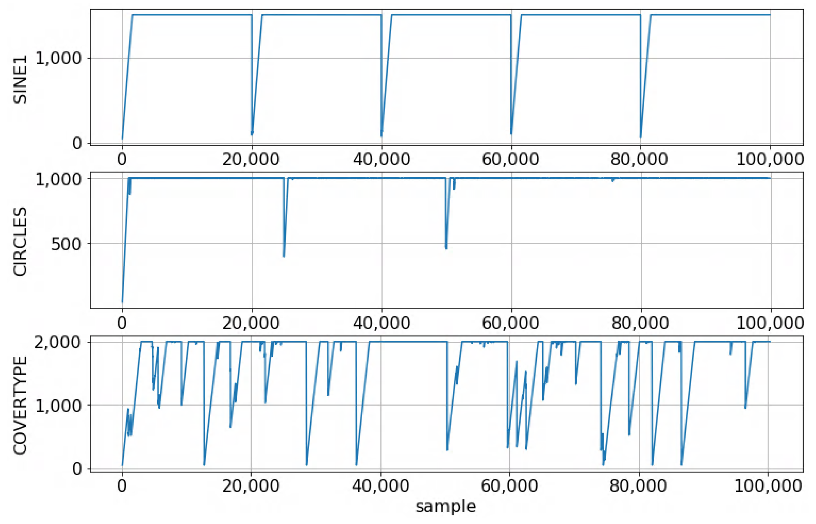
5.1. SINE1 Dataset

Following [28,30,46], we used the SINE1 synthetic dataset (https://github.com/alipsgh, accessed on 2 October 2021), with two classes, 100,000 samples, and abrupt concept drift [31]. Additionally, 10% noise was added to the data. The rationale, as given by [46], is to assess also the robustness of the drift detection classifier in the presence of noise. The dataset has only two attributes, $(x_a,x_b)$, uniformly distributed in $[0,1]$. A point with $x_b<sin\left(x_a\right)$ is classified as belonging to one class, with the rest belong to the other class. At every 20,000 instances, an abrupt drift occurs: the classification is reversed. This presents the advantage that we know exactly where drift occurs and as such, we can evaluate the sensibility of our classifier.

5.2. CIRCLES Dataset

Another dataset used frequently in the literature is the CIRCLES dataset [20,27,31,47]. It is a set with gradual drift; two attributes x and y are uniformly distributed in the interval $[0,1]$. The circle function is ${(x=x_c)}^2+{(y-y_c)}^2=r_c^2$, where $x_c$ and $y_c$ define the circle center and $r_c$ is its radius. Positive instances are inside the circle, whereas the exterior ones are labelled as negative. Concept drift happens when the classification function (the circle parameters) changes; this happens every 25,000 samples.

5.3. COVERTYPE Dataset

The Forest Covertype dataset [48] is often applied in the data stream mining literature [20,27,31,47]. It describes the forest coverage type for 30 × 30 meter cells, provided by the US Forest Service (USFS) Region 2 Resource Information System. There are 581,012 instances and 54 attributes, not counting the class type. Out of these, only 10 are continuous, so the rest of them (such as wilderness area and soil type) are nominal. The set defines seven classes; we only used two classes, the most represented, with a total of 495,141 data samples. The classes are equally balanced: 211,840 in class 1 vs. 283,301 in class 2. The dataset was already normalized [49]. For the SVM to work properly in case of small windows, we detected the sets of temporally consecutive data samples belonging to the same class. We observed that, apart from a set of 5692 consecutive elements of the same class, which was skipped, all other such sequences had less than 300 elements. For those, we switched the middle element with the most recent element of a different class, to ensure that we have no sequences longer than 150 samples from the same class. This is similar with SVM keeping its most recent sample of the opposite class, in the definition of the hyperplane.

Concept drift in the COVERTYPE case may appear as a result of change in the forest cover type [31]. There is no hard evidence of concept drift in this case; we do not know whether concept drift does occur, and in that case, what is its position within the data stream [31,47,50]. Thus we cannot compare against a baseline; only comparison among employed methods is possible.

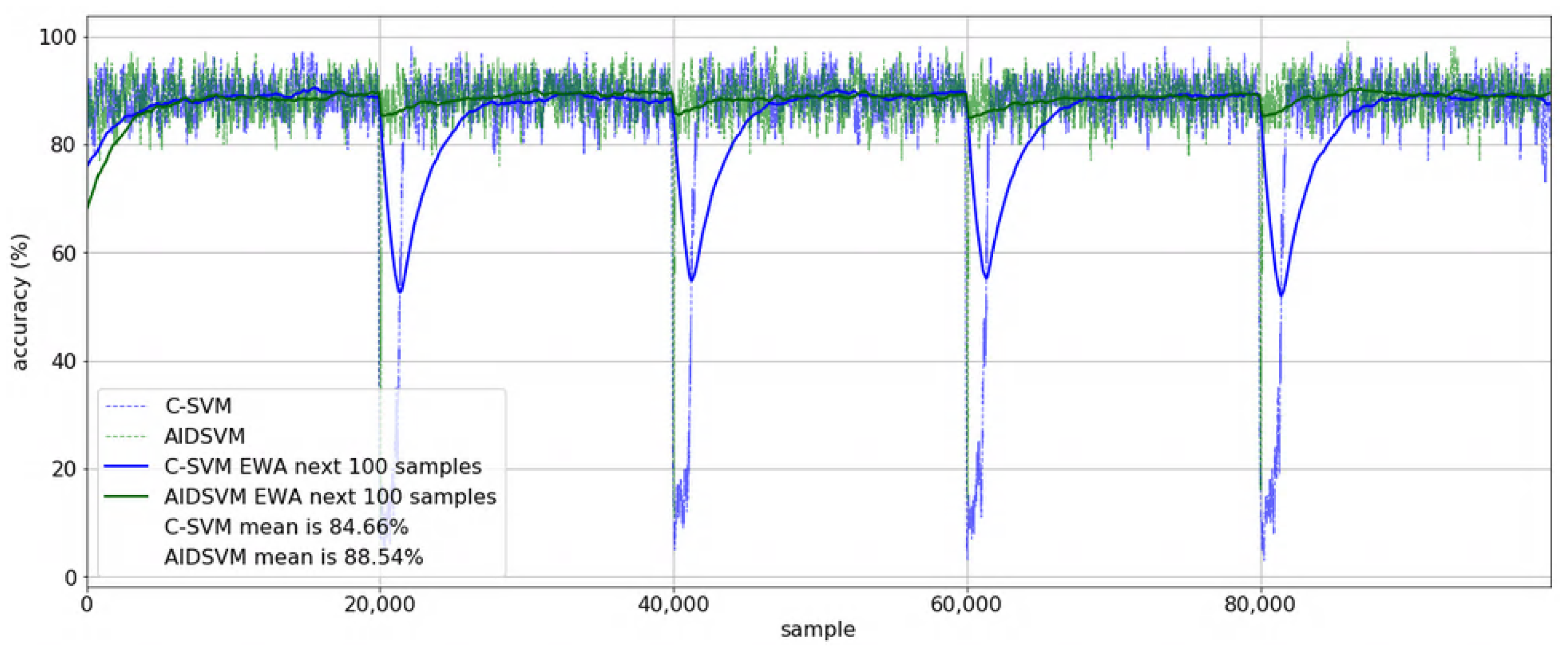
5.4. Performance Comparison

We evaluated the performance on these three datasets, for two classifiers with five drift detection methods from the Tornado framework [45] (thus a total of 10 models), against AIDSVM and C-SVM. For AIDSVM, different parameters were used, and they are dataset dependent. They are shown in

Table 1. C-SVM and AIDSVM parameters used for each data set.

Dataset	Window Size	$\mathit{\gamma }$ (gamma)	C
SINE1	1500	6.008484	10
CIRCLES	1000	7.797753	1
COVERTYPE	2000	0.241477	100

, where the window size for AIDSVM is the maximum allowed.

The window size was chosen as a sufficiently large number, that provided best accuracy results when the model was trained from the beginning of the stream and tested on the next 100 samples. The $\gamma$ parameter was computed as $\gamma =1/(N·{\sigma }^2)$, where N is the dataset size and ${\sigma }^2$ the variance for all of the features. These were previously rescaled to fit in the [0, 1] interval. The C parameter was determined by the incremental training process, sufficiently large so that the initial support vector set would not become empty. As we wanted a confidence level of 95% in the Hoeffding inequality (1), we chose $\delta =0.05$.

The accuracies for the realized experiments are presented in

Table 2. Accuracy comparison between AIDSVM and other concept drift detectors, on given datasets. C-SVM was also evaluated, although its window size is not variable.

Method on Dataset	SINE1	CIRCLES	COVERTYPE
NB+FHDDM	85.32%	86.24%	87.94%
NB+FHDDMS	85.35%	86.26%	87.05%
NB+DDM	85.06%	86.06%	88.43%
NB+EDDM	82.50%	84.81%	84.92%
NB+ADWIN	84.72%	86.20%	86.78%
HT+FHDDM	86.37%	87.16%	89.16%
HT+FHDDMS	86.36%	87.19%	87.58%
HT+DDM	86.09%	86.97%	89.90%
HT+EDDM	83.69%	85.21%	84.98%
HT+ADWIN	84.09%	86.74%	87.02%
C-SVM	84.83%	87.17%	91.79%
AIDSVM	88.68%	87.22%	92.17%

. On the SINE1 dataset, the most accurate classic drift detection model is HT+FHDDM, with 86.37%. The C-SVM performance is only 84.83%; because C-SVM is not suited for abrupt drift, this poor accuracy is somehow expected. The AIDSVM model was the best performer, with 88.68%, indicating good adaptability to abrupt drift. On the CIRCLES dataset, however, it can be seen that the best models seem to be on par—HT+FHDDM with 87.16%, HT+FHDDMS with 87.19%, C-SVM with 87.17% and AIDSVM with 87.22%. Being a dataset with gradual concept drift, C-SVM is expected to behave well, and this is supported by the experiment. For the COVERTYPE dataset, the best classic model seems to be the HT+DDM, achieving 89.90%. C-SVM performance of 91.79% suggests that this dataset seems to also be a gradual drift dataset; however, better performance of AIDSVM of 92.17% indicates a rather rapid drift.

We made a time comparison between C-SVM and AIDSVM in

Table 3. Running time comparison between C-SVM and AIDSVM, in milliseconds per training sample. Training was carried out on 5000 samples with a window size of 1000, for all datasets.

Method on Dataset	SINE1	CIRCLES	COVERTYPE
C-SVM	154 ± 12	115 ± 8	119 ± 11
AIDSVM	117 ± 7	75 ± 9	73 ± 6

. We recorded the mean time and standard deviation, in milliseconds, after training on the same 1000 sample window size, on an Intel Core i5-8400 CPU with 16 GB RAM. We observed the advantage of AIDSVM without retraining from scratch.

Figure 3 shows the window size dynamics for the three datasets, trained on the AIDSVM classifier. For SINE1, we can clearly observe the sudden drift changes; the window becomes almost empty. For the CIRCLES dataset, drift change is still visible at samples 25,000, 50,000, and only a little bit at 75,000. We explain this by considering the gradual drift employed by the dataset and by the fact that using a shifting window is inherently a way to cope with drift. In case of the COVERTYPE dataset, the drift here looks more like a combination of gradual and abrupt drifts; this is also supported by the point-to-point comparison among the drift methods contained in

Table 4. Drift points detected by the compared models. Drift is detected the same regions, mostly observed for the SINE1 and CIRCLES datasets. Here, we have only shown the first five detections. The presence of ellipsis shows that the sequence is longer. Clear concept drift is seen in SINE1 around theoretical positions 20,000, 40,000 and 60,000, and for CIRCLES at positions 25,000, 50,000 and 75,000. COVERTYPE dataset seems to have a mixture of abrupt and gradual concept drift.

Drifts Signalled	SINE1	CIRCLES	COVERTYPE
NB+FHDDM	20,048, 40,043, 60,048, 80,047	25,061, 50,063, 75,104	803, 1761, 2689, 3149, 3587 ...
NB+FHDDMS	20,033, 40,035, 60,047, 80,037	25,061, 50,023, 75,104	803, 1607, 2009, 2644, 3129 ...
NB+DDM	20,156, 40,138, 60,106, 80,171	25,339, 50,240, 75,676	839, 2105, 2717, 3149, 3588 ...
NB+EDDM	93, 21,121, 40,949, 61,038, 61,165 ...	110, 260, 31,163, 50,397, 50,629 ...	116, 280, 364, 553, 703 ...
NB+ADWIN	20,065, 26,178, 27,775, 29,924, 40,069 ...	9537, 25,090, 27,843, 50,052, 75,205 ...	1025, 2818, 3747, 4772, 5637 ...
HT+FHDDM	20,054, 40,052, 41,756, 60,052, 80,051	25,061, 50,063, 75,066	816, 1673, 2031, 2700, 3146 ...
HT+FHDDMS	20,036, 40,042, 41,765, 60,047, 80,038	25,061, 50,023, 75,066	816, 1607, 2009, 2706, 3123 ...
HT+DDM	20,150, 40,144, 60,154, 80,164	25,304, 50,297, 75,559	853, 1924, 51,532, 51,741, 51,775 ...
HT+EDDM	93, 20,899, 40,873, 60,951, 61,224 ...	110, 260, 27,840, 31,500, 31,930 ...	116, 280, 364, 553, 703 ...
HT+ADWIN	2877, 4770, 6435, 8260, 12,869 ...	1985, 5506, 25,091, 28,420, 50,053 ...	993, 2786, 4675, 5636, 5797 ...
AIDSVM	20,036, 40,041, 60,044, 80,038	25,055, 25,069, 50,023, 50,030, 50,037, 75,668 ...	990, 996, 1006, 4715, 4751 ...

.

5.5. Qualitative Discussion

We represented the instant accuracy of the classifier (given in Figure 4). This was computed as a mean on the next 100 samples. The C-SVM instant accuracy falls at concept drift and slowly recovers, whereas the AIDSVM accuracy recovers faster. We also computed the Exponentially Weighted Average at sample t, computed as $V_t=\beta V_{t-1}+(1-\beta )A_t$, where $A_t$ is the accuracy at sample t. $\beta$ is chosen to be 0.9995, equivalent to a weighted average for about the last 2000 samples. One can see that the simple C-SVM EWA drops by about 20%, whereas the AIDSVM EWA drop is below 5%. The last metric, the mean accuracy, shows that, compared with the C-SVM, the AIDSVM mean accuracy gain is about 4%; interestingly, our mean accuracy of 88.54% is slightly better than Diversity Measure as a Drift Detection Method in a semi-supervised environment (DMDDM-S, 87.2%) presented in the most recent work of Mahdi [46], on the same SINE1 dataset.

6. Conclusions

We introduced AIDSVM, an incremental–decremental SVM concept drift model with adaptive shifting window. It presents two important advantages: (i) better accuracy, because irrelevant samples are discarded at the appropriate moment based on the Hoeffding test, and (ii) it is faster than a classic SVM since no retraining is needed—the model is adapted on-the-run. The results of the experiments on three frequently used datasets indicate a better adjustment of the AIDSVM model compared to other drift-detection methods.

Experimental evaluation indicated that AIDSVM copes better with concept drift, and in general it has similar or better accuracy results compared to classical concept drift detectors. However, the construction of the incremental solution is generally slower; this makes AIDSVM well suited for data streams with moderate throughput, where good accuracy is required in the presence of concept drift. To the best of our knowledge, our implementation is the first online SVM classifier that copes with concept drift using dynamic adaptation of the shifting window by avoiding retrain from scratch.

A further improvement to the current AIDSVM implementation would be to speed up the unlearning process. This can be carried out in two stages. First, one would determine how many samples from the beginning of the window have to be removed. This is achieved by testing the Hoeffding condition (1) on sub-windows formed by successively removing the oldest sample. Second, after finding out which samples must be removed, one would have to decrease all ${\lambda }_c$ characteristic values for those vectors in a uniform way, and a similar relation to Equation (13) must be derived.

AIDSVM could be modified to support regression problems; the incremental–decremental SVM for regression was previously approached in [41,42,43]. A natural direction would also be to extend AIDSVM to multiple classes, where an ensemble of incremental SVMs with adaptive windows could be trained in parallel.

References

- Voosen, P. New climate models predict a warming surge. Science 2019, 364, 222–223. [Google Scholar] [CrossRef]
- Gama, J. Knowledge Discovery from Data Streams, 1st ed.; Chapman & Hall/CRC: Boca Raton, FL, USA, 2010. [Google Scholar]
- Lazarescu, M.M.; Venkatesh, S.; Bui, H.H. Using multiple windows to track concept drift. Intell. Data Anal. 2004, 8, 29–59. [Google Scholar] [CrossRef]
- Gama, J.; Žliobaitė, I.; Bifet, A.; Pechenizkiy, M.; Bouchachia, A. A survey on concept drift adaptation. ACM Comput. Surv. (CSUR) 2014, 46, 1–37. [Google Scholar] [CrossRef]
- Iwashita, A.S.; Papa, J.P. An overview on concept drift learning. IEEE Access 2019, 7, 1532–1547. [Google Scholar] [CrossRef]
- Lu, J.; Liu, A.; Dong, F.; Gu, F.; Gama, J.; Zhang, G. Learning under concept drift: A review. IEEE Trans. Knowl. Data Eng. 2019, 31, 2346–2363. [Google Scholar] [CrossRef]
- Farid, D.M.; Zhang, L.; Hossain, A.; Rahman, C.M.; Strachan, R.; Sexton, G.; Dahal, K. An adaptive ensemble classifier for mining concept drifting data streams. Expert Syst. Appl. 2013, 40, 5895–5906. [Google Scholar] [CrossRef]
- Ditzler, G.; Roveri, M.; Alippi, C.; Polikar, R. Learning in nonstationary environments: A survey. IEEE Comput. Intell. Mag. 2015, 10, 12–25. [Google Scholar] [CrossRef]
- Alippi, C.; Qi, W.; Roveri, M. Learning in nonstationary environments: A hybrid approach. In Proceedings of the International Conference on Artificial Intelligence and Soft Computing, Zakopane, Poland, 11–15 June 2017; pp. 703–714. [Google Scholar]
- Raab, C.; Heusinger, M.; Schleif, F.M. Reactive Soft Prototype Computing for Concept Drift Streams. Neurocomputing 2020, 416, 340–351. [Google Scholar] [CrossRef]
- Saigal, P.; Khanna, V. Multi-category news classification using Support Vector Machine based classifiers. SN Appl. Sci. 2020, 2, 458. [Google Scholar] [CrossRef]
- Shamshirband, S.; Esmaeilbeiki, F.; Zarehaghi, D.; Neyshabouri, M.; Samadianfard, S.; Ghorbani, M.A.; Mosavi, A.; Nabipour, N.; Chau, K. Comparative analysis of hybrid models of firefly optimization algorithm with support vector machines and multilayer perceptron for predicting soil temperature at different depths. Eng. Appl. Comput. Fluid Mech. 2020, 14, 939–953. [Google Scholar] [CrossRef]
- Dabija, A.; Kluczek, M.; Zagajewski, B.; Raczko, E.; Kycko, M.; Al-Sulttani, A.H.; Tardà, A.; Pineda, L.; Corbera, J. Comparison of Support Vector Machines and Random Forests for Corine Land Cover Mapping. Remote Sens. 2021, 13, 777. [Google Scholar] [CrossRef]
- Flores, C.; Taramasco, C.; Lagos, M.E.; Rimassa, C.; Figueroa, R.A. Feature-Based Analysis for Time-Series Classification of COVID-19 Incidence in Chile: A Case Study. Appl. Sci. 2021, 11, 7080. [Google Scholar] [CrossRef]
- Zhu, H.; Woo, J.H. Hybrid NHPSO-JTVAC-SVM Model to Predict Production Lead Time. Appl. Sci. 2021, 11, 6369. [Google Scholar] [CrossRef]
- Shabani, S.; Samadianfard, S.; Sattari, M.T.; Mosavi, A.; Shamshirband, S.; Kmet, T.; Várkonyi-Kóczy, A.R. Modeling Pan Evaporation Using Gaussian Process Regression K-Nearest Neighbors Random Forest and Support Vector Machines. Comparative Analysis. Atmosphere 2020, 11, 66. [Google Scholar] [CrossRef]
- Klinkenberg, R.; Joachims, T. Detecting concept drift with support vector machines. In Proceedings of the Seventeenth International Conference on Machine Learning (ICML ’00), Stanford, CA, USA, 29 June–2 July 2000; ICML: San Diego, CA, USA, 2000; pp. 487–494. [Google Scholar]
- Klinkenberg, R. Learning drifting concepts: Example selection vs. example weighting. Intell. Data Anal. 2004, 8, 281–300. [Google Scholar] [CrossRef]
- Sun, J.; Li, H.; Adeli, H. Concept Drift-Oriented Adaptive and Dynamic Support Vector Machine Ensemble With Time Window in Corporate Financial Risk Prediction. IEEE Trans. Syst. Man Cybern. Syst. 2013, 43, 801–813. [Google Scholar] [CrossRef]
- Bifet, A.; Gavaldà, R. Learning from time-changing data with adaptive windowing. In Proceedings of the Seventh SIAM International Conference on Data Mining (SDM’07), Minneapolis, MN, USA, 26–28 April 2007; Volume 7, p. 6. [Google Scholar]
- Gemaque, R.N.; Costa, A.F.J.; Giusti, R.; dos Santos, E.M. An overview of unsupervised drift detection methods. WIREs Data Min. Knowl. Discov. 2020, 6, e1381. [Google Scholar] [CrossRef]
- Elwell, R.; Polikar, R. Incremental learning in nonstationary environments with controlled forgetting. In Proceedings of the 2009 International Joint Conference on Neural Networks, Atlanta, GA, USA, 14–19 June 2009; pp. 771–778. [Google Scholar]
- Elwell, R.; Polikar, R. Incremental learning of concept drift in nonstationary environments. IEEE Trans. Neural Netw. 2011, 22, 1517–1531. [Google Scholar] [CrossRef] [PubMed]
- Shen, Y.; Zhu, Y.; Du, J.; Chen, Y. A Fast Learn++.NSE classification algorithm based on weighted moving average. Filomat 2018, 32, 1737–1745. [Google Scholar] [CrossRef]
- Gomes, H.M.; Bifet, A.; Read, J.; Barddal, J.P.; Enembreck, F.; Pfharinger, B.; Holmes, G.; Abdessalem, T. Adaptive random forests for evolving data stream classification. Mach. Learn. 2017, 106, 1469–1495. [Google Scholar] [CrossRef]
- Gama, J.; Medas, P.; Castillo, G.; Rodrigues, P.P. Learning with drift detection. In Proceedings of the 17th Brazilian Symposium on Artificial Intelligence (SBIA 2004), Sao Luis, Maranhao, Brazil, 29 September–1 October 2004. [Google Scholar]
- Baena-Garcıa, M.; del Campo-Ávila, J.; Fidalgo, R.; Bifet, A.; Gavalda, R.; Morales-Bueno, R. Early drift detection method. In Proceedings of the Fourth International Workshop on Knowledge Discovery from Data Streams, San Francisco, CA, USA; 2006; Volume 6, pp. 77–86. [Google Scholar]
- Pesaranghader, A.; Viktor, H.L. Fast Hoeffding drift detection method for evolving data streams. In Proceedings of the Joint European Conference on Machine Learning and Knowledge Discovery in Databases, Riva del Garda, Italy, 19–23 September 2016; pp. 96–111. [Google Scholar]
- Pesaranghader, A.; Viktor, H.L.; Paquet, E. A framework for classification in data streams using multi-strategy learning. In International Conference on Discovery Science; Springer: Cham, Switzerland, 2016; pp. 341–355. [Google Scholar] [CrossRef]
- Pesaranghader, A.; Viktor, H.; Paquet, E. Reservoir of diverse adaptive learners and stacking fast Hoeffding drift detection methods for evolving data streams. Mach. Learn. J. 2018, 107, 1711–1743. [Google Scholar] [CrossRef]
- Pesaranghader, A. A Reservoir of Adaptive Algorithms for Online Learning from Evolving Data Streams. Ph.D. Dissertation, University of Ottawa, Ottawa, ON, Canada, 2018. [Google Scholar] [CrossRef]
- Yan, M.M.W. Accurate detecting concept drift in evolving data streams. ICT Express 2020, 6, 332–338. [Google Scholar] [CrossRef]
- ZareMoodi, P.; Siahroudi, S.K.; Beigy, H. A support vector based approach for classification beyond the learned label space in data streams. In Proceedings of the 31st Annual ACM Symposium on Applied Computing (SAC ’16), Pisa Italy, 4–8 April 2016; Association for Computing Machinery: New York, NY, USA, 2016; pp. 910–915. [Google Scholar]
- Yalcin, A.; Erdem, Z.; Gurgen, F. Ensemble based incremental SVM classifiers for changing environments. In Proceedings of the 2007 22nd International Symposium on Computer and Information Sciences, Ankara, Turkey, 7–9 November 2007; pp. 1–5. [Google Scholar]
- Altendeitering, M.; Dübler, S. Scalable Detection of Concept Drift: A Learning Technique Based on Support Vector Machines. In Proceedings of the 30th International Conference on Flexible Automation and Intelligent Manufacturing (FAIM2021), Athens, Greece, 15–18 June 2021; Volume 51, pp. 400–407. [Google Scholar]
- Cauwenberghs, G.; Poggio, T. Incremental and decremental support vector machine learning. In Proceedings of the 13th International Conference on Neural Information Processing Systems (NIPS’00), Denver, CO, USA, 1 January 2000; MIT Press: Cambridge, MA, USA; 2000; pp. 388–394. [Google Scholar]
- Diehl, C.P.; Cauwenberghs, G. SVM incremental learning, adaptation and optimization. In Proceedings of the International Joint Conference on Neural Networks, Portland, OR, USA, 20–24 July 2003; Volume 4, pp. 2685–2690. [Google Scholar]
- Laskov, P.; Gehl, C.; Krüger, S.; Mxuxller, K. Incremental support vector learning: Analysis, implementation and applications. J. Mach. Learn. Res. 2006, 7, 1909–1936. [Google Scholar]
- Gâlmeanu, H.; Andonie, R. Implementation issues of an incremental and decremental SVM. In Proceedings of the 18th International Conference on Artificial Neural Networks (ICANN ’08), Prague, Czech Republic, 3–6 September 2008; Part I; Springer: Berlin/Heidelberg, Germany, 2008; pp. 325–335. [Google Scholar]
- Gâlmeanu, H.; Andonie, R. A multi-class incremental and decremental SVM approach using adaptive directed acyclic graphs. In Proceedings of the 2009 International Conference on Adaptive and Intelligent Systems, Klagenfurt, Austria, 24–26 September 2009; pp. 114–119. [Google Scholar]
- Martin, M. On-line support vector machine regression. In Machine Learning: ECML 2002; Elomaa, T., Mannila, H., Toivonen, H., Eds.; Springer: Berlin/Heidelberg, Germany, 2002; pp. 282–294. [Google Scholar]
- Ma, J.; Theiler, J.; Perkins, S. Accurate on-line support vector regression. Neural Comput. 2003, 15, 2683–2703. [Google Scholar] [CrossRef]
- Gâlmeanu, H.; Sasu, L.M.; Andonie, R. Incremental and decremental SVM for regression. Int. J. Comput. Commun. Control 2016, 11, 755–775. [Google Scholar] [CrossRef]
- Ma, Y.; Zhao, K.; Wang, Q.; Tian, Y. Incremental cost-sensitive Support Vector Machine with linear-exponential loss. IEEE Access 2020, 8, 149899–149914. [Google Scholar] [CrossRef]
- Pesaranghader, A. The Tornado Framework for Data Stream Mining (Python Implementation). Available online: https://github.com/alipsgh/tornado (accessed on 3 October 2021).
- Mahdi, O.A.; Pardede, E.; Ali, N.; Cao, J. Fast Reaction to Sudden Concept Drift in the Absence of Class Labels. Appl. Sci. 2020, 10, 606. [Google Scholar] [CrossRef]
- Huang, D.T.J.; Koh, Y.S.; Dobbie, G.; Bifet, A. Drift detection using stream volatility. In Joint European Conference on Machine Learning and Knowledge Discovery in Databases; Springer: Berlin/Heidelberg, Germany, 2015; pp. 417–432. [Google Scholar]
- Blackard, J.A.; Dean, D.J. Comparative accuracies of artificial neural networks and discriminant analysis in predicting forest cover types from cartographic variables. Comput. Electron. Agric. 2000, 24, 131–151. [Google Scholar] [CrossRef]
- Centre for Open Software Innovation, The University of Waikato. Datasets—MOA. 2019. Available online: https://moa.cms.waikato.ac.nz/datasets/ (accessed on 1 May 2020).
- Bifet, A.; Kirkby, R. Data Stream Mining: A Practical Approach; MOA, The University of Waikato, Centre for Open Software Innovation: Hamilton, New Zealand, 2009; Available online: https://www.cs.waikato.ac.nz/~abifet/MOA/StreamMining.pdf (accessed on 2 October 2021).