Research on Wind Field Characteristics Measured by Lidar in a U-Shaped Valley at a Bridge Site

Abstract

Currently, research on wind fields of U-shaped valleys is rarely reported, and anemometers or wind observation towers are usually used for field measurement, but the measured position is limited and the cost is high. In order to study the wind characteristics in a mountainous U-shaped valley, a long-range, all-weather, high-precision Wind3D 6000 lidar was placed at a bridge site located in a U-shaped valley. Then, according to the data effective ratio and wind speed, nearly 6 months of original data ranging from 0 m to 810 m were analyzed statistically. It was found that the spatio-temporal distribution of wind speed and direction is obviously not uniform, and the wind parameters are correlated among different virtual wind towers (VWTs). By classification, the effective data of midspan position is taken as the research object, and the wind speed profile is divided into three categories. Type-1 shows disorderly characteristics; Type-2 shows a linear relationship; and Type-3 shows a nonlinear relationship. The wind direction is consistent with the main wind direction at the bridge site and the average wind direction of different VWTs has a high consistency. The concept of wind-direction deflection rate is put forward to describe the variation of wind direction with height. These measured wind parameters could be used as a reference for bridge wind-resistant design.

1. Introduction

Many long-span bridges have been built in mountainous valley areas, for example, Royal Gorge Bridge, (1929, 384 m), Cañon City, Colorado, USA; Aizhai Bridge (2012, 1176 m), Hunan Province, China; Longjiang Bridge (2016, 1196 m), Yunnan Province, China; and Yachihe Bridge (2016, 800 m), Guizhou Province, China; and more will be built in the future. The requirement for long-span bridges in mountainous valley areas also enhances the performance standard of long-span bridges. Among them, the influence of wind on the design, construction, and operation of long-span bridges cannot be ignored, and is even one of the control factors. At the same time, the distribution of wind parameters in mountainous valley terrain is different from that in open and flat terrain, and is extremely complex, as shown in Figure 1. From the perspective of wind speed, the wind speed profile in flat and open areas conforms to the law of power index or logarithm. Although much research has been conducted in this field, the spatio-temporal distribution of wind speed in mountainous valley areas has its own unique patterns, which are generally analyzed on a case-by-case basis and are difficult to be described by a unified mathematical model. In addition, due to the impact of topographic relief and elevation changes, the gradient wind height in mountain valleys may be higher than the former. At present, the study of wind parameters in mountainous valley areas is one of the hot topics in wind engineering research.

The research on mountainous valley wind parameters by scholars mainly applies the methods of wind tunnel terrain model test, numerical simulation, and field measurement. Wind tunnel terrain model test is widely used, but there is room for improvement in accuracy because of characteristic flow simulation and scaling model making [1,2,3]. With the development of computer technology and computational fluid dynamic (CFD), numerical simulation methods have been applied more and more widely, and their reliability has also been verified [4,5,6]. However, further research is needed in calculating domain size and setting boundary conditions, such as surface roughness. In spite of the time consuming, huge investment and limited measured positions, field measurement can obtain the most direct and reliable wind field data, and it is often used as the verification standard for the analysis results of the first two methods [7,8,9,10,11,12,13].

From the perspective of measuring equipment performance, field measurement can be divided into direct measurement and indirect measurement. Direct measurements, for example, tall mast balloons with anemometers have been important in defining the profiles of atmospheric parameters of the atmosphere boundary layer [11,12,13,14,15,16,17]. The ability to observe atmospheric variables with a minimum of assumptions has been widely used, despite the development costs and associated limitations on sample size. However, limited by the performance of direct measurement instruments, only limited monitoring positions can be set up, and the location of instruments is restricted by terrain and other conditions; therefore, direct instruments are generally installed on the bridge deck of pylons. This method is difficult to use to obtain wide-range wind parameters at bridge sites, such as the wind profile at the bridge midspan located at deep mountainous valley. Especially in the design state, when the bridge has not been built yet, it is impossible to conduct large-scale direct observation in a mountainous valley.

With the development of testing technology, especially the application of remote monitoring technology, indirect observation is mostly made by remote sensors, such as radar, sodar, and lidar, which greatly reduce the cost of field measurement and allow a large range of massive data to be obtained. Owing to the advantages of volume sampling, remote sensors are becoming more widely recognized, and the availability of improved resolution and Doppler capabilities in these remote sensors have greatly increased their utility, thus making remote sensors the observational platform of choice in many situations. [3,18,19,20,21,22,23,24,25].

Among the remote sensors, lidar is uniquely capable of collecting an all-weather, high-accuracy, large detection range high, spatio-temporal resolution and other excellent characteristics, and is a more powerful instrument for measuring wind parameters than others. Charland [26] used the Doppler wind lidar (DWL)to research a wildland fire plume in complex terrain east of San Jose, CA, USA. Vertical wind and turbulence profiles within 200 m were measured to study the kinematic structure and spatial and temporal evolution of the fire plume and found that the velocity accelerates at the plume boundary. Liao et al. [24] used the data measured by a WindCube lidar installed in mountain valley and turbulence characteristics of the wind were analyzed. Wang [27] et al. studied the wind characteristics in a mountainous valley by 2D anemometers and 3D Doppler radar.

At present, the measured research on wind parameters of mountainous valleys at bridge site areas mostly adopts anemometers or anemometer mast. The spatial range of the measured data is limited, and it is difficult to arrange multiple wind towers in the spanning direction of the bridge due to the constraints of terrain and equipment. There are limited reports about the wind field measurement study of U-shaped valleys through lidar. The aim of this paper is to obtain the wind characteristics at a bridge site in a U-shaped valley and provide a reference for the wind-resistant design of related bridges in similar valleys. Therefore, in this paper, a high performance Wind3D 6000 lidar was used to study the wind field characteristics in a U-shaped valley at bridge site. Five virtual wind towers were set up at the key position of the main girder for continuous observation for about six months. Then, through screening the original data, the measured data in the range of 0–810 m were analyzed, and wind speed and direction were analyzed from the perspectives of time, space, and statistical distribution. The research method and results can provide reference for the study of mountain canyon wind fields, and it provides a wind parameter basis for bridge design.

2. Topography Description and Field Measurement Setup

2.1. Topography Description

A U-shaped valley is located in the Jinsha River (Lijiang, Yunnan Province, China) under the jurisdiction of southwest China, with numerous peaks and ravines crisscrossing, low latitude and high altitude, and topographic features and profiles of a U-shaped valley, as showed in Figure 2. Its climate is dominated by the northern subtropical montane monsoon climate. In addition, the main wind direction in this region is southwesterly year round, and gale weather appears from November to April. A long-span suspension bridge will cross the U-shaped valley, with an elevation of about 2000 m and a height of about 600 m above the river, as shown in Figure 2. With the lidar as the center, the altitude changes from 1380 m to 3480 m in the area with a radius of 5 km, as shown in Figure 3.

2.2. Lidar System

Compared with traditional wind measurement means, such as anemometers and sodar, the Wind3D 6000 3D scanning wind measuring lidar has the advantages of higher measurement accuracy, higher spatial and temporal resolution, and lower detection blind area. An optical scanning mirror is equipped with high-pointing accuracy, 3D scanning detection can be realized, and the maximum detection radius can be up to 6 km. In addition, the lidar has the advantages of small size, lightweightedness, and low power consumption, which makes it easy to build stations and transport in the field, as shown in Figure 4.

The Wind3D 6000 3D scanning wind measuring lidar is a coherent wind measuring lidar system, which is mainly composed of a laser transmitting and scanning subsystem, a receiving subsystem, a real-time signal processing subsystem, a communication subsystem, etc., as shown in Figure 5. The radial velocity is calculated through the principle of optical pulse coherent Doppler frequency shift detection. On the other hand, based on the assumption of the horizontal homogeneous wind speed [28,29], the boundary layer wind profile is inversed by the microbeam system, with visibility data also provided.

The lidar emits an eye-safe invisible light with a wavelength of 1550 nm and transmits laser pulses into the atmosphere at a rate of 1–10 Hz, which is user-definable. The Wind3D 6000 lidar equipped an optical scanner enabling scans from 0–360° azimuth angles and −90–270° pitch angles, and there are up to 398 user-defined range gates at 15 m spacing, with the minimum range at 45 m and the maximum range at 6000 m. In addition, various scan models are available; for example, range–height indicator (RHI), plan position indicator (PPI), Doppler beam swinging (DBS), and so on. RHI is used in this paper to obtain wind speed and direction profiles, as detailed in

Table 1. Performance indicators of the lidar.

Numbers	Indicators	Description
1	Radial Detection Range	45–6000 m
2	Radial Range Resolution	15 m/30 m/User Defined
3	Laser Wavelength	1550 nm, Invisible and Safe to Human Eyes
4	Data Refresh Frequency	1 Hz–10 Hz
5	Range of Radial Measured Wind Speed	0–75 m/s
6	Range of Wind Direction	0–360°
7	Accuracy of Wind Speed	≤0.1 m/s
8	Accuracy of Wind Direction	<3°
9	Scan Modes	RHI/ PPI/ DBS/ VAD/ Scripting
10	Range of Servo Scanning	Horizontal Direction: 0–360°, Vertical Scanning: 90–270°
11	Weight	<90 kg
12	Size Length/Width/Height	638 mm /626 mm /907 mm
13	Power Supply	220 V/50 Hz
14	Communication Mode	Ethernet/3G/4G/Modbus

.

2.3. Setup of the Lidar

The setup of the lidar system is divided into site selection, measuring scheme, installation, debugging, and testing. The details are as follows:

(1)

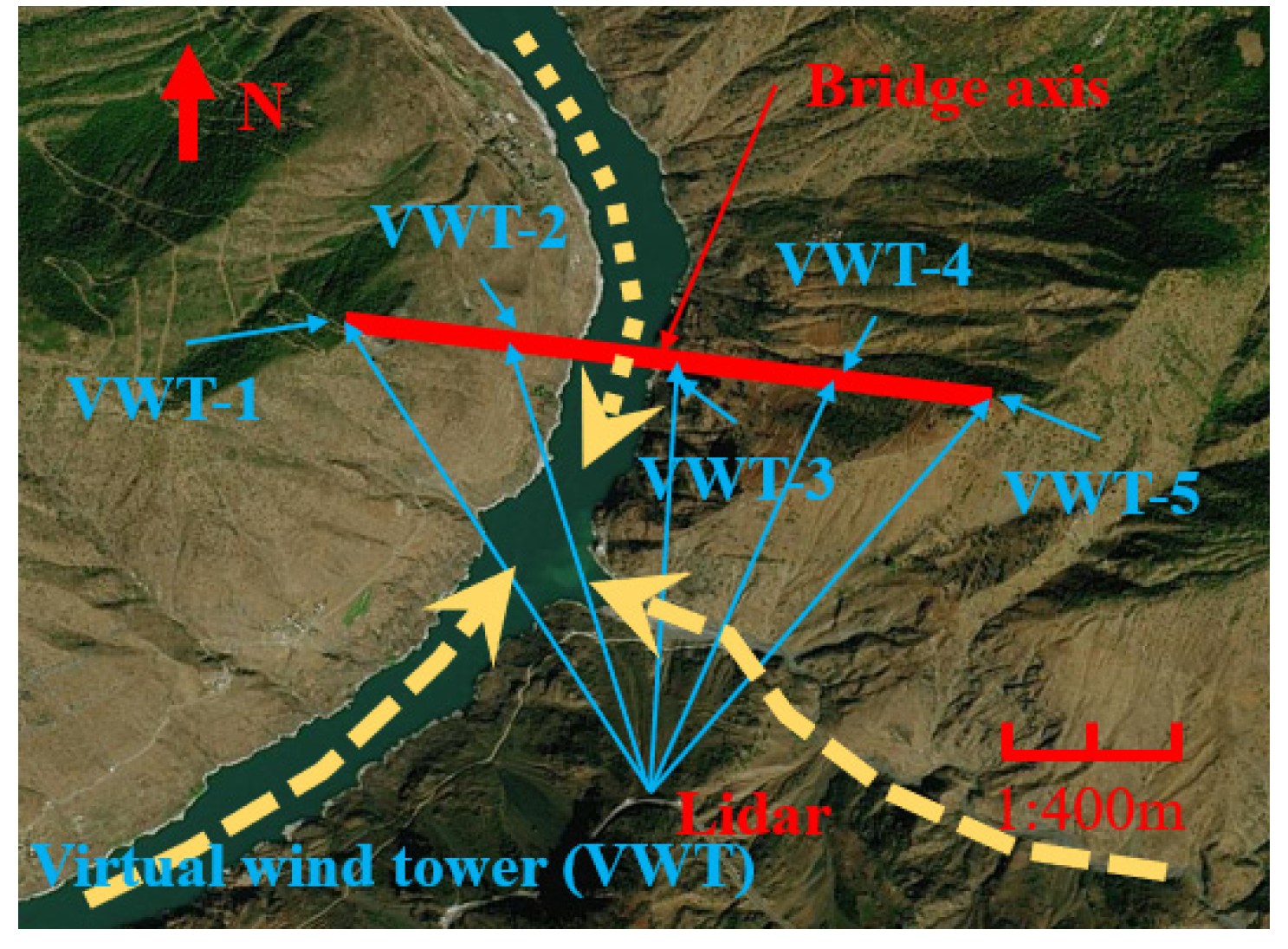
Site selection: After a detailed field investigation, the lidar is installed beside the highway. The site is open and unobstructed, the horizontal distance from the midspan of the bridge is about 1700 m, and the vertical height difference is about 200 m, which is convenient for transportation and field electricity consumption, as shown in Figure 2 and Figure 3.

(2)

Measuring scheme: In order to measure the distribution characteristics of wind parameters in the spanning direction of the bridge, measuring points are arranged at 5 key positions: the west bridge tower, 1/4 span, midspan, 3/4 span, and east bridge tower, respectively. Five virtual wind measuring towers are set up, namely from VWT-1 to VWT-5, as shown in Figure 2.

(3)

Installation: the lidar system is equipped with a power supply, monitoring, and a 4G network to facilitate data transmission and site monitoring, as shown in Figure 5.

(4)

Debugging: after field debugging, with little interference from the surrounding environment, the signal-to-noise ratio (SNR) is greater than 10, the lidar system runs normally, and the wind parameter measurement is normal and reliable.

(5)

Testing: according to the gale wind season from 11 November 2020 to 3 May 2021, from late autumn to early summer, the operating state of the lidar system was real-time monitored, and a continuous 173 days of data was measured and recorded.

3. Raw Data Validity

The effective distance of the lidar pulse signal is related to weather conditions, especially the aerosol content in the air, such as rain, snow, fog, and haze, which may change the aerosol content and affect the transmission of the echo signal. In order to improve the quality and reliability of the data, the following screening work was performed for the original data before data analysis:

(1)

Abnormal value data shall be removed; that is, when the wind speed or direction exceeds its measurement range of 0–75 m/s or 0–360°, the wind speed or direction is “999”, and it shall be removed.

(2)

Eliminate unreliable data. According to the suggestions of the equipment manufacturer, the larger the SNR, the more reliable the data will be. When the SNR is less than 10 dB, there may be strong noise and disturbance, which will reduce the reliability of the measured data, so the data shall be eliminated.

(3)

Conduct data validity analysis for data with good continuity and reliability within the scope of concern, such as 0–810 m.

The data effective ratio is defined as follows: Taking 24 h per day as the unit time, the total numbers of wind speed data at different heights and the total numbers of data excluded are counted to obtain the total numbers of effective data. Then, the total numbers of effective data are divided by the total numbers of data to obtain the effective ratio of data at different heights, as shown in Equation (1).

$$\beta =\frac{N-N_{error}}{N}$$

(1)

where $\beta$ is the effective ratio, $N$ is the total numbers of data at a measured height in a day, and $N_{error}$ is the total numbers of excluded data at a measured height in the day.

As can be seen from Figure 6 and

Table 2. Historical weather list.

Date	Weather	Wind Direction	Effective Ratio β Range
19 December 2020	Cloudy	South Wind Grade 2	0.382–0.919
20 January 2021	Light Rain	Southwest Wind Grade 2	0.134–0.726
5 March 2021	Light Rain	West Wind Grade 1	0.263–0.794
25 March 2021	Clear Day	Southwest Wind Grade 2	0.772–0.992
10 April 2021	Fine Day	Southwest Wind Grade 2	0.692–0.980

, the measurement range of the lidar is between 0–810 m per day, and the effective ratio of the data fluctuates greatly. Combined with historical weather forecasts, it was light rain on 20 January and 5 March, the data efficiency was the worst, and the data efficiency of each height was less than 0.8. It was cloudy on 19 December and the data quality was better than that on 20 January. On 25 March the day was clear and the effective ratio varied from 0.772 to 0.992 and had good performance. It can be found that lidar data has a higher quality when measured on a fine day. This may help to improve the application efficiency of lidar based on weather forecasts.

4. Results and Discussion

4.1. Wind Speed

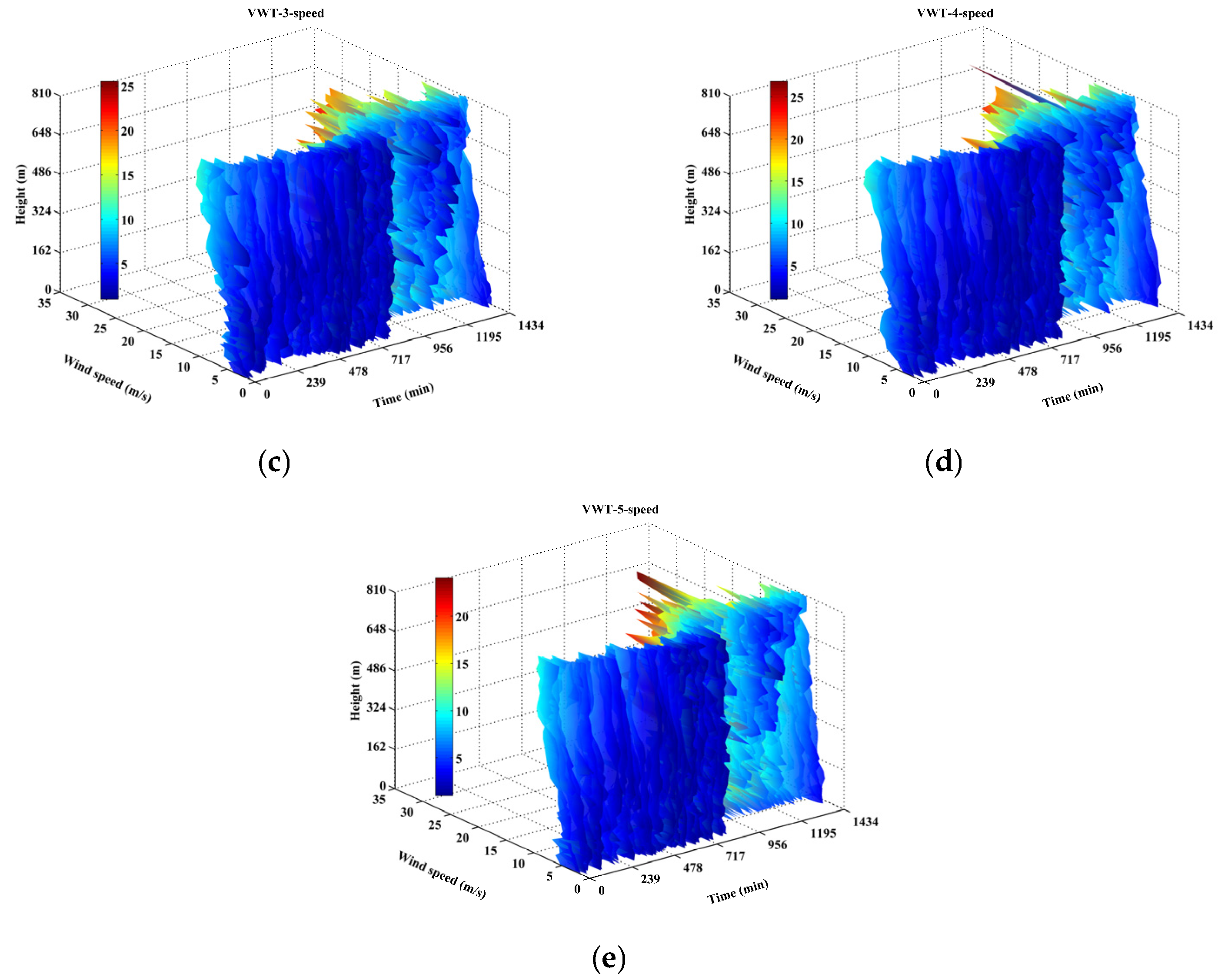
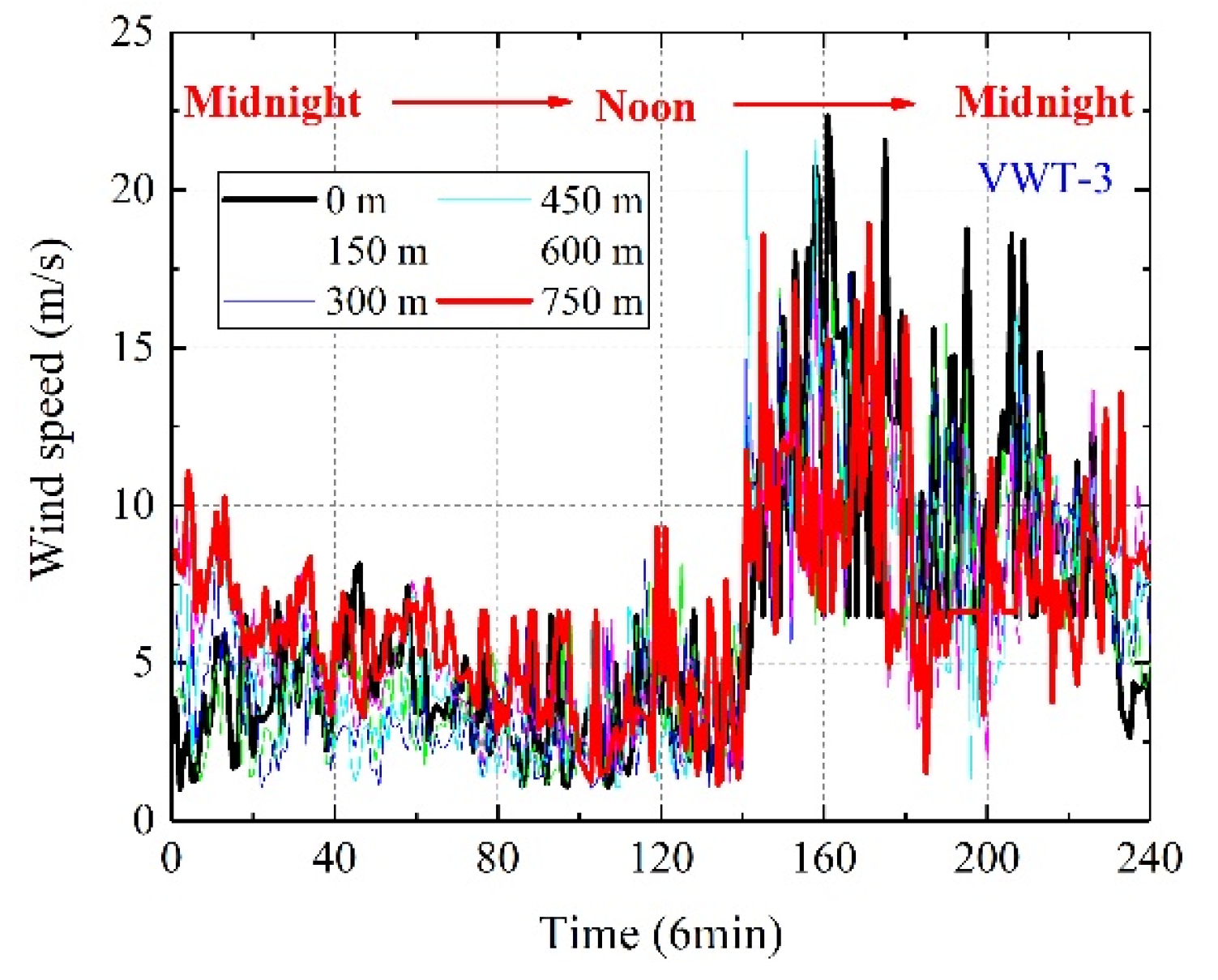
4.1.1. Wind Speed Distribution

Wind speed spatio-temporal distribution and time history at a certain height are shown in Figure 7. It can be found that the wind speed varies from 0 m/s to 25 m/s. Although the spatio-temporal distribution of the wind speed at the same location of the virtual wind tower (VWT) is obviously nonuniform, its trend among different virtual towers is consistent to a certain extent, which indicates that wind speed distribution along the spanning direction of the bridge has a certain correlation.

Time history of the wind speed is shown in Figure 8, with the height of the bridge deck taken as the starting point, from 0 m to 750 m and the interval is 150 m; thus, 6 specific heights are selected. The starting point on the time axis is selected as 0:0:0 at midnight every day, and the day is divided into 240 time periods with an interval of 6 min. Taking the third category as an example, the wind speed at different heights fluctuates significantly, and the degree of fluctuation does not decrease significantly with the increase in height, indicating that the influence of mountain valley terrain on the wind speed is more obvious than that of surface roughness.

After preliminary research, it was found that during the measurement period, the datawith the wind speed effective ratio is not less than 0.6, occupied only 8%. On the one hand, when wind speed is low, the noise proportion of the original data is relatively high, and the reliability of the data is relatively low. On the other hand, the influence of small value wind on wind-resistance performance of the structure is negligible. Then, combined with the data characteristics, 57% of the data is excluded with a minimum wind speed not less than 7 m/s as the standard. Next, the effective wind speed at different virtual tower locations was counted, and it was found that the effective data at the midspan location accounted for 34%, much higher than other measuring positions. Due to the influence of valley topography, the effective data at the west bridge tower accounted for the lowest proportion, only 11%. Furthermore, the effective data at VWT-3 was taken as the research object and analyzed, as showed in Figure 9.

In wind-resistance research of long-span bridges, the wind speed at the height of main girder deserves special attention [30] and is set as the reference wind speed, which is used to process the dimensionless wind speed.

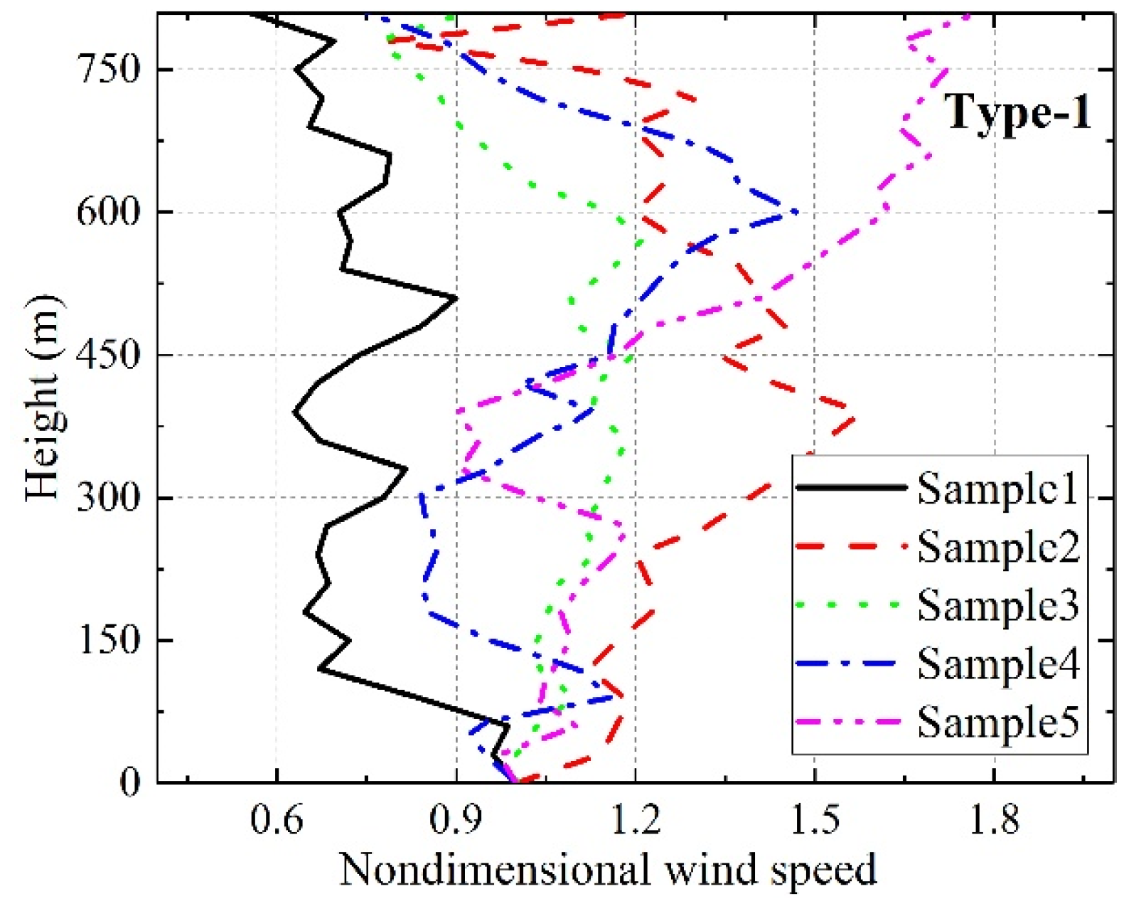
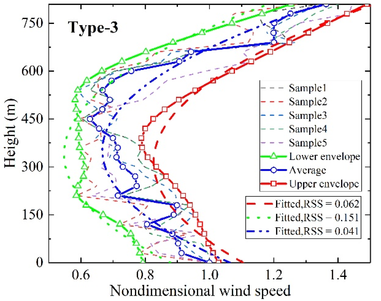
4.1.2. Wind Speed Profile

After analysis, the nondimensional wind speed profiles do not conform to the power or exponential law and are classified into three types, as shown from Figure 10, Figure 11 and Figure 12, respectively. According to the shape characteristics of the wind profile, Equations (2) and (3) are used for the nondimensional wind profile fitting.

$$h=au+\overline{h}$$

(2)

where $u$ is the nondimensional wind speed, $h$ is the height (m), and $a$ and $\overline{h}$ are the parameters (m).

$$H=h_{\ast }\pm \eta \sqrt{u-\overline{u}}$$

(3)

where $H$ and $h_{\ast }$ are the height (m), $u$ and $\overline{u}$ are the nondimensional wind speed, and $\eta$ is the coefficient of surface roughness (m).

The first type, Type-1, takes up the highest proportion at 62%, and it is discrete and has no obvious rule. The second type, Type-2, has approximately linear distribution and the nondimensional wind speed in the whole measuring space does not change significantly with height, which is basically the same as the wind speed at the bridge deck. The third type, Type-3, is characterized by a relatively high wind speed at the bridge deck position as the height rises to about 400 m and the nondimensional wind speed decreases by about 20%, presenting an increasing trend. The piecewise exponential function is used for fitting, and the result is shown in the Equation (3).

$$h_{Upper}=16200.0u-16637.40$$

$$h_{Average}=18837.21u-18592.30$$

$$h_{Lower}=23142.86u-21731.15$$

$$H_{Upper}=357.14\pm 597.61\sqrt{u-0.75}$$

$$H_{Average}=312.50\pm 559.02\sqrt{u-0.75}$$

$$H_{Lower}=344.83\pm 587.22\sqrt{u-0.54}$$

4.2. Wind Direction

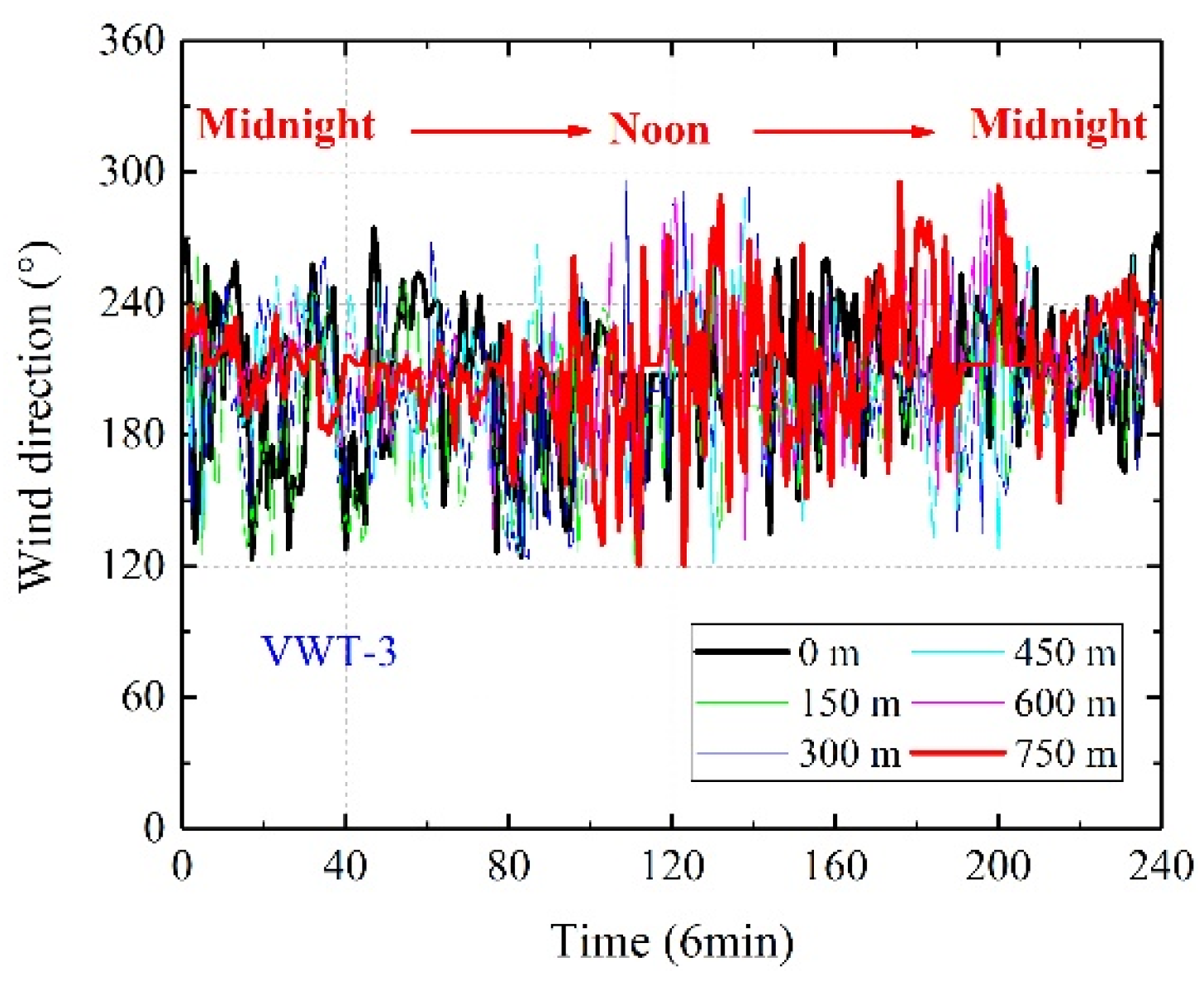
4.2.1. Wind-Direction Distribution

During the measurement period, the data of a certain day with a higher data effective ratio was selected to analyze. The spatio-temporal distribution of wind direction at the locations of the 5 virtual wind towers was shown in Figure 13. Overall, the wind direction ranges from 120° to 300°, with southerly wind dominating, which is consistent with the annual main wind direction at the bridge site. Wind direction changes with time, height, and position in a complex way, and it is difficult to find a uniform rule.

Taking VWT-3 as an example, 6 specific heights were selected. Figure 14 shows the time-history change of wind direction at this position. It can be roughly seen that wind-direction fluctuation decreases with the increase in height, reflecting that the interference of a U-shaped valley to incoming flow gradually decreases with height.

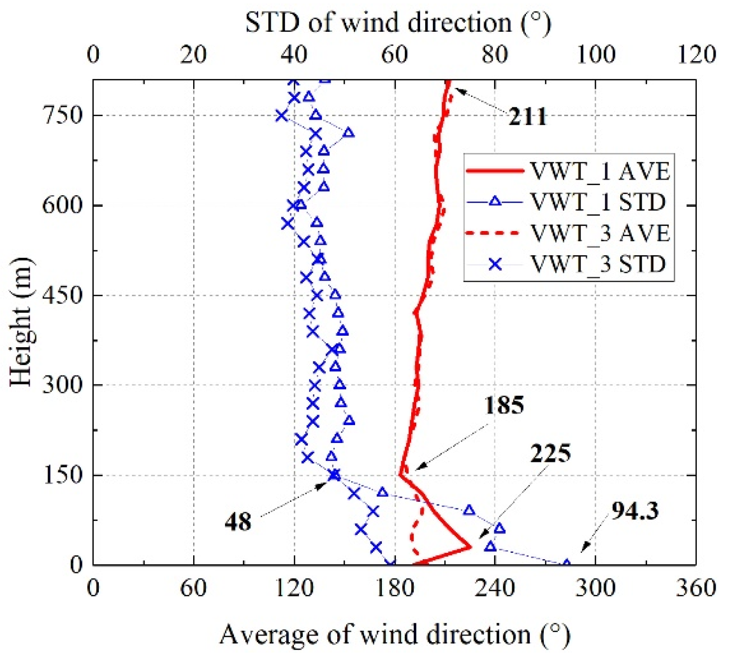
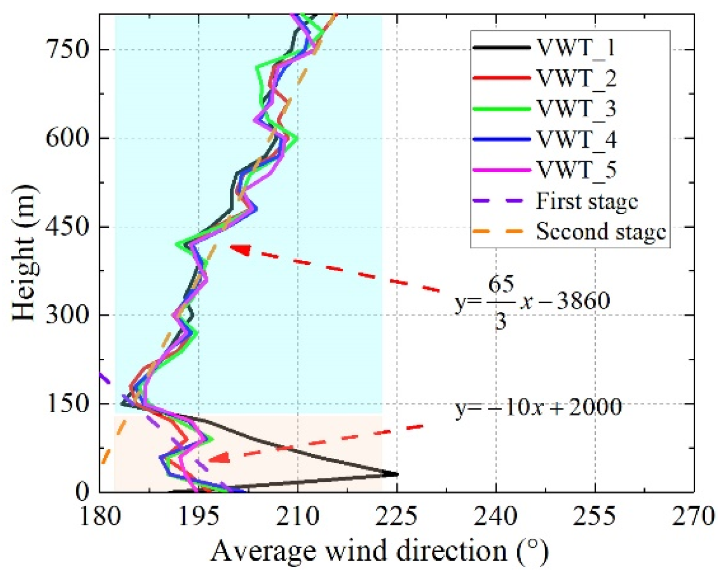
4.2.2. Wind-Direction Deflection

Taking the midspan position as an example from Figure 15, the wind direction rose, and it can be seen that the wind direction at the bridge deck height is significantly affected by the U-shaped valley terrain, and the wind direction is highly dispersed, mainly north and southeast. As height rises, the wind direction dispersion decreases, and the main wind turns to the right and tends to the southwest. In order to study the torsion law of wind direction with height, the following analysis was made:

First, the wind-direction deflection rate $\alpha$ is defined: the wind direction of the oncoming flow would deflect with height due to the influence of U-shaped valley topography, Coriolis force, and other factors, which is represented as the change rate of the angle with the unit height. The smaller the absolute value $\alpha$ is, the more violently the oncoming wind direction is deflected by disturbance, as shown in Figure 16 and Equation (4).

$$\alpha =\frac{{\partial }_y}{{\partial }_x}$$

(4)

Take the derivative of Equation (4),

$$y=\alpha x+b$$

(5)

where $x$ is the wind-direction angle (°), $y$ is the height (m), $\alpha$ is the wind-direction deflection rate (m/°), and $b$ is the undetermined constant (m).

Further, 24 h is taken as the unit time to calculate the average (AVE) and standard deviation (STD) of the wind direction. Taking VWT-1 and VWT-3 as examples, as shown in Figure 17, the 150 m height is the turning point, and the AVE and STD of wind direction have a numerical mutation, which may be due to the blocking effect range of mountains in the direction of incoming flow being about 150 m. On the one hand, below 150 m, the maximum AVE wind direction is about 225° and the maximum STD is about 94.3°. On the other hand, above 150 m, the AVE and STD of wind direction fluctuate weakly; the AVE wind direction increases about 14%, from 185° to 211°, and the STD of wind direction goes down by 8°and 4°.

Next, taking 150 m as the cutoff point, the data is divided into two parts, the first stage and the second stage. Statistical and fitting analysis was made for the AVE wind direction. Deflection of wind direction with height is treated as a linear piecewise function, as shown in Figure 18 and Equation (5).

$$y=\{\begin{array}{c}-10x+200(x\le 185)\\ 65x/3-3860(185<x\le 245.5)\end{array}$$

The fitting results are shown in Figure 18 and Equation (5). The wind-direction deflection pattern shows two linear relations of positive and negative. Below the height turning point in the first stage, the wind deflection rate ${\alpha }_1$ is −10, and in the second stage, the wind deflection rate ${\alpha }_2$ is 65/3, $\left|{\alpha }_2\right|\approx 2.17\left|{\alpha }_{{}_1}\right|$ According to the definition of $\alpha$,below 150 m, the wind deflection is more dramatic, approximately 2.17 times that above the cutoff point.

5. Conclusions

(1)

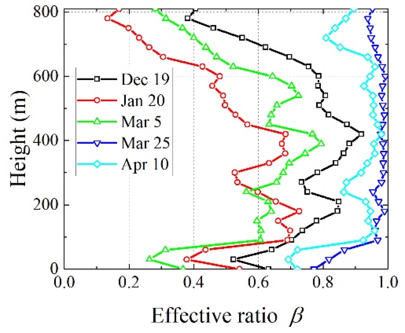
Lidar can measure and record wind parameters in the field for a long time, and in view of the effective ratio $\beta$, measurements taken can obtain higher quality data when the weather is clear.

(2)

The wind field data during the measuring period were selected and analyzed, and it is found that the wind field parameter showed nonuniform characteristics in time and height.

(3)

The nondimensional wind speed profile was divided into three types (mussy, linear, and piecewise exponential pattern), and the regularity of power exponent is not obvious. The three types are different from those recommended in the specification or those in an open area.

(4)

The wind direction has a certain consistency at different VWTs, and the phenomenon of wind direction twists with the height could be described by the wind-direction deflection rate $\alpha$. In addition, below the cutoff point, the wind deflection is more dramatic.

(5)

According to the distribution pattern of wind speed and direction, wind parameters could be applied to bridge design; for example, wind speed and distribution along the bridge deck or wind-direction change along the pylon, and these could be further. discussed.

(6)

Confined to the performance of the lidar, no analysis has been performed on wind speed power spectrum and spatial coherence, and further updates of equipment or advanced analysis method is needed.

References

1. Bowen, A. Modelling of strong wind flows over complex terrain at small geometric scales. J. Wind Eng. Ind. Aerodyn. 2003, 91, 1859–1871. [Google Scholar] [CrossRef]
2. Chen, T.; Li, Y.; Luan, D.; Jiao, A.; Yang, L.; Fan, C.; Shi, L. Study of flow characteristics in tunnels induced by canyon wind. J. Wind Eng. Ind. Aerodyn. 2020, 202, 104236. [Google Scholar] [CrossRef]
3. Song, J.-L.; Li, J.-W.; Flay, R.G. Field measurements and wind tunnel investigation of wind characteristics at a bridge site in a Y-shaped valley. J. Wind Eng. Ind. Aerodyn. 2020, 202, 104199. [Google Scholar] [CrossRef]
4. Blocken, B.; Persoon, J. Pedestrian wind comfort around a large football stadium in an urban environment: CFD simulation, validation and application of the new Dutch wind nuisance standard. J. Wind Eng. Ind. Aerodyn. 2009, 97, 255–270. [Google Scholar] [CrossRef]
5. Blocken, B.; van der Hout, A.; Dekker, J.; Weiler, O. CFD simulation of wind flow over natural complex terrain: Case study with validation by field measurements for Ria de Ferrol, Galicia, Spain. J. Wind Eng. Ind. Aerodyn. 2015, 147, 43–57. [Google Scholar] [CrossRef]
6. Hu, P.; Li, Y.; Han, Y.; Cai, S.C.S.; Xu, X. Numerical simulations of the mean wind speeds and turbulence intensities over simplified gorges using the SST k-ω turbulence model. Eng. Appl. Comput. Fluid Mech. 2016, 10, 359–372. [Google Scholar] [CrossRef] [Green Version]
7. Hui, M.; Larsen, A.; Xiang, H. Wind turbulence characteristics study at the Stonecutters Bridge site: Part I—Mean wind and turbulence intensities. J. Wind Eng. Ind. Aerodyn. 2009, 97, 22–36. [Google Scholar] [CrossRef]
8. Bastos, F.; Caetano, E.; Cunha, Á.; Cespedes, X.; Flamand, O. Characterisation of the wind properties in the Grande Ravine viaduct. J. Wind Eng. Ind. Aerodyn. 2018, 173, 112–131. [Google Scholar] [CrossRef]
9. Pirooz, A.A.S.; Flay, R.G.J. Comparison of Speed-Up Over Hills Derived from Wind-Tunnel Experiments, Wind-Loading Standards, and Numerical Modelling. Boundary-Layer Meteorol. 2018, 168, 213–246. [Google Scholar] [CrossRef]
10. Lystad, T.M.; Fenerci, A.; Øiseth, O.A. Evaluation of mast measurements and wind tunnel terrain models to describe spatially variable wind field characteristics for long-span bridge design. J. Wind Eng. Ind. Aerodyn. 2018, 179, 558–573. [Google Scholar] [CrossRef]
11. Zhang, J.; Zhang, M.; Li, Y.; Fang, C. Comparison of wind characteristics at different heights of deep-cut canyon based on field measurement. Adv. Struct. Eng. 2019, 23, 219–233. [Google Scholar] [CrossRef]
12. Jing, H.; Liao, H.; Ma, C.; Tao, Q.; Jiang, J. Field measurement study of wind characteristics at different measuring positions in a mountainous valley. Exp. Therm. Fluid Sci. 2020, 112, 109991. [Google Scholar] [CrossRef]
13. Al-Jiboori, M.H.; Xu, Y.; Qian, Y. Local Similarity Relationships In The Urban Boundary Layer. Boundary-Layer Meteorol. 2002, 102, 63–82. [Google Scholar] [CrossRef]
14. Al-Jiboori, M.; Hu, F. Surface Roughness Around a 325-m Meteorological Tower and Its Effect on Urban Turbulence. Adv. Atmos. Sci. Engl. Version 2005, 22, 595–605. [Google Scholar] [CrossRef]
15. Wood, C.R.; Lacser, A.; Barlow, J.F.; Padhra, A.; Belcher, S.E.; Nemitz, E.; Helfter, C.; Famulari, D.; Grimmond, C.S.B. Turbulent Flow at 190 m Height Above London During 2006–2008: A Climatology and the Applicability of Similarity Theory. Boundary-Layer Meteorol. 2010, 137, 77–96. [Google Scholar] [CrossRef] [Green Version]
16. Ye, Z.; Li, N.; Zhang, F. Wind characteristics and responses of Xihoumen Bridge during typhoons based on field monitoring. J. Civ. Struct. Heal. Monit. 2019, 9, 1–20. [Google Scholar] [CrossRef]
17. Yu, C.; Li, Y.; Zhang, M.; Zhang, Y.; Zhai, G. Wind characteristics along a bridge catwalk in a deep-cutting gorge from field measurements. J. Wind Eng. Ind. Aerodyn. 2019, 186, 94–104. [Google Scholar] [CrossRef]
18. Tamura, Y.; Suda, K.; Sasaki, A.; Iwatani, Y.; Fujii, K.; Hibi, K.; Ishibashi, R. Wind speed profiles measured over ground using Doppler sodars. J. Wind Eng. Ind. Aerodyn. 1999, 83, 83–93. [Google Scholar] [CrossRef]
19. Tamura, Y.; Iwatani, Y.; Hibi, K.; Suda, K.; Nakamura, O.; Maruyama, T.; Ishibashi, R. Profiles of mean wind speeds and vertical turbulence intensities measured at seashore and two inland sites using Doppler sodars. J. Wind Eng. Ind. Aerodyn. 2007, 95, 411–427. [Google Scholar] [CrossRef]
20. Frehlich, R.; Kelley, N. Measurements of Wind and Turbulence Profiles With Scanning Doppler Lidar for Wind Energy Applications. IEEE J. Sel. Top. Appl. Earth Obs. Remote Sens. 2008, 1, 42–47. [Google Scholar] [CrossRef]
21. Sjöholm, M.; Courtney, M.; Enevoldsen, K.; Lindelöw, P.; Mann, J.; Mikkelsen, T. Remote Sensing of the 3D Wind and Turbulence Field by Coherent Doppler Lidars for Wind Power Applications. In Proceedings of the 2008 AGU Fall Meeting, San Francisco, CA, USA, 15–19 December 2008. [Google Scholar]
22. Canadillas, B.; Westerhellweg, A.; Neumann, T. Testing the performance of a ground-based wind LiDAR system: One year intercomparison at the offshore platform FINO1. DEWI-Magazin 2011, 38, 58–64. [Google Scholar]
23. Kogaki, T.; Sakurai, K.; Shimada, S.; Kawabata, H.; Otake, Y.; Kondo, K.; Fujita, E. Field Measurements of Wind Characteristics Using LiDAR on a Wind Farm with Downwind Turbines Installed in a Complex Terrain Region. Energies 2020, 13, 5135. [Google Scholar] [CrossRef]
24. Liao, H.; Jing, H.; Ma, C.; Tao, Q.; Li, Z. Field measurement study on turbulence field by wind tower and Windcube Lidar in mountain valley. J. Wind Eng. Ind. Aerodyn. 2020, 197, 104090. [Google Scholar] [CrossRef]
25. Knoop, S.; Bosveld, F.C.; de Haij, M.J.; Apituley, A. A 2-year intercomparison of continuous-wave focusing wind lidar and tall mast wind measurements at Cabauw. Atmospheric Meas. Tech. 2021, 14, 2219–2235. [Google Scholar] [CrossRef]
26. Charland, A.M. Doppler Wind Lidar Observations of a Wildland Fire Plume. Master’s Thesis, San Jose State University, San Jose, CA, USA, August 2012. [Google Scholar]
27. Wang, F.; Chen, X.; He, R.; Liu, Y.; Hao, J.; Li, J. Wind Characteristics in Mountainous Valleys Obtained through Field Measurement. Appl. Sci.-Basel 2021, 11, 7717. [Google Scholar] [CrossRef]
28. Stull, R.B. Boundary Layer Clouds; Springer: Amsterdam, The Netherlands, 1988. [Google Scholar]
29. Young, G.S. Convection in the atmospheric boundary layer. Earth-Sci. Rev. 1988, 25, 179–198. [Google Scholar] [CrossRef]
30. Tang, H.; Li, Y.; Shum, K.; Xu, X.; Tao, Q. Non-uniform wind characteristics in mountainous areas and effects on flutter performance of a long-span suspension bridge. J. Wind Eng. Ind. Aerodyn. 2020, 201, 104177. [Google Scholar] [CrossRef]
Figure 1. Difference in wind speed between open and mountainous valley terrain.
Applsci 11 09645 g001
Figure 2. Terrain features and bridge.
Applsci 11 09645 g002
Figure 3. Terrain contour line.
Applsci 11 09645 g003
Figure 4. Diagram of the lidar.
Applsci 11 09645 g004
Figure 5. Diagram of Wind3D 6000 lidar wind measuring system. (a) Contour line at bridge site, (b) Wind3D 6000 Lidar system.
Applsci 11 09645 g005
Figure 6. Data effective ratio.
Applsci 11 09645 g006
Figure 7. Spatio-temporal distribution of wind speed, (a) VWT-1; (b) VWT-2; (c) VWT-3; (d) VWT-4; (e) VWT-5.
Applsci 11 09645 g007aApplsci 11 09645 g007b
Figure 8. Time history of wind speed.
Applsci 11 09645 g008
Figure 9. Flow chart of the raw data selection.
Applsci 11 09645 g009
Figure 10. Wind speed profile of Type-1.
Applsci 11 09645 g010
Figure 11. Wind speed profile of Type-2.
Applsci 11 09645 g011
Figure 12. Wind speed profile of Type-3.
Applsci 11 09645 g012
Figure 13. Spatio-temporal distribution of wind direction, (a) VWT-1; (b) VWT-2; (c) VWT-3; (d) VWT-4; (e) VWT-5.
Applsci 11 09645 g013
Figure 14. Time history of wind direction.
Applsci 11 09645 g014
Figure 15. Wind direction rise diagram at VWT-3.
Applsci 11 09645 g015
Figure 16. Sketch of wind-direction deflection rate.
Applsci 11 09645 g016
Figure 17. Average and STD of wind direction.
Applsci 11 09645 g017
Figure 18. The law of wind direction changes with height.
Applsci 11 09645 g018