A Comparison Study on the Improved Operation Strategy for a Parabolic trough Solar Power Plant in Spain

Abstract

The present work focuses on the development of a detailed dynamic model of an existing parabolic trough solar power plant (PTSPP) in Spain. This work is the first attempt to analyse the dynamic interaction of all parts, including solar field (SF), thermal storage system (TSS) and power block (PB), and describes the heat transfer fluid (HTF) and steam/water paths in detail. Advanced control circuits, including drum level, economiser water bypass, attemperator and steam bypass controllers, are also included. The parabolic trough power plant is modelled using Advanced Process Simulation Software (APROS). An accurate description of control structures and operation strategy is necessary in order to achieve a reasonable dynamic response. This model would help to identify the best operation strategy due to DNI (direct normal irradiation) variations during the daytime. The operation strategy used in this model has also been shown to be effective compared to decisions made by operators on cloudy periods by improving power plant performance and increasing operating hours.

1. Introduction

Solar power plants are a very important factor in the countries that depend on renewable energy sources for their energy system because they can also produce electrical power in the night. Current estimates of the amount of power supplied by solar thermal power plants in the world are at approximately 6.2 GW by 2020. For example, in Spain there are 2.3 GW produced by 47 parabolic trough power plants, 51 MW by three solar power plants and 31 MW by two linear Fresnel power plants.

There are 2.194 GW under construction around the world [1,2]. The estimated power is expected to reach more than 11 GW by 2030 depending on an average development of the CSP technology. Approximately 15% of these power plants will be installed in Europe, 30% in northern Africa and 55% in the Middle East [3,4,5,6].

In the following study, an overview of the dynamic simulation models for parabolic trough power plants will be presented that have been implemented in the past to improve and evaluate methods for increasing the operational flexibility of these plants. Due to DNI and demand variations, the use of dynamic models is of great importance. These variations in the performance need to use the transient solution of three conservation laws (energy, mass and momentum), dynamic conditions, controllers and accompanied parts.

There are several commercial programs for power plant modelling used in solar thermal applications, namely TRNSYS, EcoSimPro, EBSILON Professional, IPSEpro, GATECYCLE, MATHEMATICA, DYMOLA and APROS [5,7,8].

In general, there are few researchers who have studied the dynamic simulation of parabolic trough power plants. In particular, most researchers have not addressed optimising the performance of these plants. For this reason, we will review the most important works that have dealt with parabolic trough power plants.

Masero et al. [9] developed a control predictive model to optimise thermal power on a large scale for solar parabolic trough plants. The power plant is divided into several subsystems. They are controlled by their loop control valves to improve the performance and reduce the computation time of control inputs. The operation strategy is evaluated by decentralised and centralised control predictive models in two simulated solar fields. Frejo and Camacho [10] optimised the solar field of a parabolic trough power plant using a centralised predictive model. The best operating strategy of the power plant is implemented by regulating a group of control valves installed at the beginning of each collector loop. This leads to improving the response obtained from classic control processes for this type of power plant. The implemented control model is applied for a small parabolic trough power plant. The simulated control models are evaluated based on the data of the collector of solar fields for ACUREX (Almería, Spain) over two hours. The results of the suggested algorithm showed a good agreement with the centralised algorithm. Sánchez et al. [11] performed a control predictive model for analysis of deconcentrating control for different collector loops. The HTF temperature is controlled by deconcentrating two and four collector loops in different cases. The results showed better performance when four complexes were not concentrated in addition to maintaining the deconcentrating procedures in the areas with high control power. Montañés et al. [12] developed dynamic models of a 50 MW parabolic trough power plant using Modelica language to assess the behaviour of stored energy and its mechanism of action with the solar field (SF) and the power block (PB). The steady-state results were compared with the original plant data. Regarding dynamic behaviour, the response of the PB showed good behaviour because the chosen days were clear. Larrain et al. [13] implemented a thermal model to evaluate the reserve part required for 100 MW_el hybrid-fossil-solar PTSPP. The performance was predicted and its usefulness was explored in aiding suitable site selection among four sites. García et al. [14] provided a dynamic model of a PTSPP without power block simulation using Wolfram’s Mathematica 7 programme. The model deals only with the thermal oil behaviour within the SF and TSS. The results were compared with experimental data for a 50 MW_el of PTSPP in Spain during summer. Diendorfer et al. [15] dynamically simulated the optical performance of the collector platform. The floating stability of the existing platform design was experimentally verified, and the performance influence to go offshore was small. Schenk et al. [16] dynamically implemented a model PTSPP by DYMOLA. A transient behaviour was evaluated for the start-up case based on thermal oil behaviour. This model was checked with the Ebsilon model since there were no experimental data to investigate the model. Luo et al. [17] built a dynamic parabolic trough collector model and validated it depending on the photothermal conversion process for a parabolic trough technology. Together with the verified model with pumps, the thermal oil/water heat exchangers and other existing components, a solar field was simulated.

The review research reveals that most modelling studies found in the literature are focused on the work of specific parts of the PTSPP, such as the solar field or the thermal storage system or the power block during certain periods (clear periods). In addition, they do not address the operation of the control units and the operational strategy used in these power plants.

In this work, a detailed dynamic model of the PTSPP (Andasol II) with all control circuits is developed employing (APROS) software. The dynamic behaviour of the investigated power plant is assessed during a strongly cloudy day. The solar data is computed depending on satellite measurements and databases from ground weather stations.

Specifically, the novelty of this study can be summarised as follows:

• A detailed dynamic model of a PTSPP, including the SF, the TSS, and the PB, has been extended based on our previous studies presented. In addition, the dynamic behaviour of the thermal oil path of the power plant during heavily cloudy days in summer is discussed. The steam behaviour in the high pressure (HP)/low pressure (LP) turbine stages is also investigated. Such dynamic simulation modelling cannot be found in the literature.
• This model can also determine the best operating strategy of the power plant, taking into account the DNI variations during the day, compared to the decisions made by operators in the absence of a dynamic modelling approach.
• For model validation, the simulation results for the most important properties of the solar field, storage system, and power block are compared with measurements. The comparative work is of great interest to designers of PTSPP and scientific researchers.

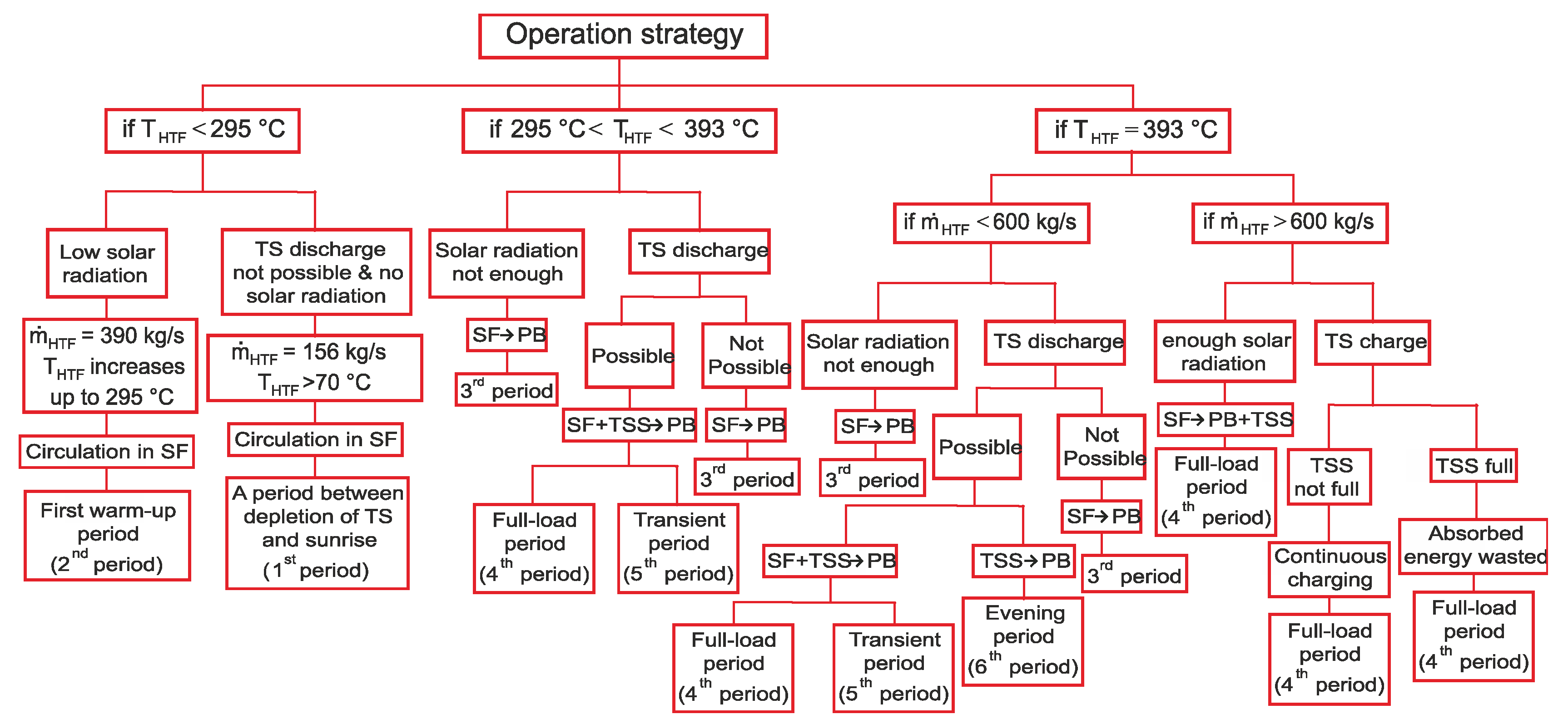
2. Power Plant Operation Strategy in Dynamic Simulation

The operation strategy performed in the dynamic simulation of the parabolic trough power plant for a single day can be defined based on six operation periods, as explained below and depicted in Figure 1:

• The first period is the period between the time of thermal storage depletion and sunrise.
• The second period represents the first warm-up period of HTF, when the HTF temperature in the SF reaches the designated temperature at the inlet (295 °C).
• The third period corresponds to the second warm-up period of HTF, where the temperature of HTF in the SF achieves the designated temperature at the outlet (393 °C).
• The fourth period represents a full-load operation period during the daytime.
• The fifth period represents the transient period that precedes the sunset.
• The sixth period is the evening period, where the thermal storage is discharged until it is completely depleted.

This operation strategy carried out in the dynamic simulation model represents the best approach comparing with the operator decisions implemented in the Andasol II.

During the first and the sixth periods (night periods), the dynamic model checks firstly whether the thermal storage discharge is available, taking into consideration the boundary conditions of the power plant. If the discharge mode is available, the power plant produces electrical power (48 MWth). On the other hand, the HTF is not circulated in the solar field. Thermal storage continues discharging during night hours until stored energy is depleted.

Conversely, when the thermal storage discharge is not available, electrical power is not produced by the steam turbine. The HTF is still circulated by the recirculation pumps within the SF at 1 kg/s for one loop as long as the design inlet temperature (295 °C) is not achieved. When the thermal oil temperature at the outlet of each loop decreases lower than 70 °C (minimum input value when there is no solar radiation or stored energy), the HTF protection system is activated to prevent the thermal oil temperature in the SF from dropping below a specified minimum temperature.

The second period (first HTF warm-up period) starts when the sun rises and continues until the designated temperature at the inlet (295 °C) is reached. After sunrise, the thermal oil in the SF is circulated with mass flow of 390 kg/s until the designate inlet temperature (295 °C) is reached. During this period the thermal oil is not transferred to the PB as the useful thermal power in the SF is still equal to zero.

Subsequently, the third period (second HTF warm-up period) begins when the design inlet temperature (295 °C) is achieved. Thereafter, the temperature and mass flow of HTF will increase together, where the design outlet temperature (393 °C) is first achieved and then the nominal value of mass flow (600 kg/s). This amount of thermal oil mass flow sent to the PB must not exceed its limit value (600 kg/s) in order to avoid the production of more steam than required. It is worth mentioning that the useful thermal energy is sent to the PB on the HTF in this period. Coinciding with the third period, the start-up period of steam turbine starts until the steam production reaches its nominal value (55 kg/s).

The assumptions implemented in the dynamic model of PTSPP are made to simulate the measured data curves for a 50 MW_el PTSPP, located in Spain. The simulation indicates an excellent agreement compared to the experimental data collected from Andasol II.

The fourth period (full-load operation period) begins after the second warm-up period of HTF, where the design conditions of HTF (600 kg/s and 393 °C) are reached at the power block inlet. This period continues during daytime until sunset. Under high DNI conditions the specified conditions of HTF are achieved, and the surplus of HTF is transferred to the TSS to start the charge phase. When the TSS is completely charged, i.e., maximum TSS capacity of 1025 MW_th h is reached, some SCAs are faced to the ground (stow mode) in order to avoid a further increase in the collected thermal energy.

Optionally, the nominal HTF mass flow can be reduced below 600 kg/s when clouds prevent the DNI from falling on a number of loops. In this case, the thermal storage is discharged, if possible, in order to maintain the target heat flow to the PB. The storage discharge period can be classified during the daylight into cases: first, if the thermal oil mass flow in the SF continues decreasing from 600 kg/s down to a minimum value of 312 kg/s, a part of the HTF coming from the PB is redirected to the thermal storage system and the rest of the thermal oil is sent to the solar field. If the DNI is still low, the operation strategy proceeds to maintain the thermal oil mass flow at a designated minimum value of 312 kg/s. Here, the power plant is operated by transferring all the useful thermal power absorbed within the SF to the PB and compensating the rest of HTF from the thermal storage system if a discharge mode is available.

Once the HTF mass flow in the SF falls below a minimum value of 312 kg/s due to the decrease in solar radiation, the designated temperature of thermal oil at the PB inlet is changed to 377 °C instead of 393 °C, and the nominal mass flow of thermal oil remains unaltered at 600 kg/s. As a result, if the mass flow of thermal oil in the SF continues falling to zero, the TSS supplies the nominal thermal power (125.75 MW_th) similar to the night period, as long as the storage discharge is possible. In this mode, 600 kg/s of HTF are directed to the TSS heat exchangers, hence no HTF is circulated in the solar field.

Whenever thermal storage discharge is not possible and there is a lack of DNI, the PB is stopped, and the thermal oil is circulated in the SF at 1 kg/s as in the first period. Hence, if the turbine is stopped several times during daytime hours because of cloudy periods, the HTF will be warmed up again which in turn leads to a second start-up process. Therefore, several start-ups can occur during the day depending on meteorological data. After the clouds pass over, the HTF can be routed to the solar field again and the process repeats starting from the third phase, as explained above.

The fifth phase (transient period) starts when the HTF mass flow falls to a value of 312 kg/s during the sunset period. The designated HTF temperature at the SF outlet is altered from 393 °C to 377 °C and the PB is operated based on the stored energy until the complete depletion of the TSS.

Fossil fuel is used in the real power plant when there is no energy stored in the storage system. However, the fossil fuel backup system has not been included in the APROS model for the results obtained in this study since the data of the real fossil fuel backup system were not available.

Finally, this operation strategy is applied in the validated power plant model for the cloudy summer day selected in this study.

3. Simulation Programme

Dynamic simulation can be a useful tool for determining the design of a new power plant, as well as to aid selection of the best operating strategy. The investigation of the dynamic behaviour of thermal power plants needs a detailed description of the thermal processes. The large fluctuations that occur during the operation of solar power plants require the use of a large number of controllers. Therefore, the process of controlling a specific property is complex, and for the purpose of achieving long-term dynamic simulation of a power plant it requires sophisticated modelling programs that include numerical solutions as well as solving differential conservation correlations.

Andasol II plant is modelled by APROS software. This programme consists of many components and different solutions which can be used for dynamic simulation. APROS implements the dynamic simulation based on homogenous and heterogeneous flow models.

Different approaches for the modelling of two-phase flow in a thermal power plant can be found in the literature, such as mixture-flow and six-equation flow models. In the mixture-flow model, the three characteristic fluid variables are calculated, including local pressure, total mass flow, and temperature or enthalpy, which are represented by three conservation equations (mass, momentum and energy) of the mixture:

Mass balance:

$$\frac{\partial \rho }{\partial t}+\frac{\partial \left(\rho u\right)}{\partial z}=0$$

(1)

Momentum balance:

$$\frac{\partial \left(\rho u\right)}{\partial t}+\frac{\partial \left(\rho u^2\right)}{\partial z}+\frac{\partial p}{\partial z}=F_{grav}+F_w$$

(2)

Energy balance:

$$\frac{\partial \left(\rho h\right)}{\partial t}+\frac{\partial \left(\rho uh\right)}{\partial z}=\frac{\partial p}{\partial t}+Q_w$$

(3)

Here, $\rho$ denotes the density of the flow mixture, $u$ represents the longitudinal velocity of fluid, $p$ and $h$ refer to the static pressure and overall enthalpy, respectively. The parameters $Q_w, F_{grav} \mathrm{and} F_w$ represent the heat transfer across the walls, the gravitational force and the friction force, respectively.

The six-equation model is more suitable for certain applications because it allows the inclusion of thermodynamic non-equilibrium states in the formulation. Here, two sets of conservation equations are formulated to determine the mass, momentum and energy balance for each phase:

Mass balance:

$$\frac{\partial \left({\chi }_k{\rho }_k\right)}{\partial t}+\frac{\partial \left({\chi }_k{\rho }_k{u}_k\right)}{\partial z}={\Gamma }_k$$

(4)

Momentum balance:

$$\frac{\partial \left({\chi }_k{\rho }_k{u}_k\right)}{\partial t}+\frac{\partial \left({\chi }_k{\rho }_k{u}_k^2\right)}{\partial z}+{\chi }_k\frac{\partial p}{\partial z}={\Gamma }_k{u}_{ik}+{\chi }_k{F}_{grav,k}+F_{wk}+F_{ik}+F_{va}+F_{fl}+\Delta P_{pu}$$

(5)

Energy balance:

$$\frac{\partial \left({\chi }_k{\rho }_k{h}_k\right)}{\partial t}+\frac{\partial \left({\chi }_k{\rho }_k{u}_k{h}_k\right)}{\partial z}={\chi }_k\frac{\partial p}{\partial t}+{\Gamma }_k{h}_{ik}+Q_{wk}+Q_{ik}+F_{ik}{u}_{ik}$$

(6)

The symbol $k$ is either $l$ = liquid or $g$ = gas, the indices $i$ and $w$ refer to the interface of two phases and the wall, respectively. The variable $\Gamma$ denotes the mass transfer rate between the phases. The parameters $F_{va}, F_{fl} \mathrm{and} ∆P_{pu}$ are valve friction, friction loss and head difference of pump, respectively. The coefficient $h$ in Equation (6) is the overall enthalpy which includes the kinetic energy and $Q_{ik}$ is the heat transfer at the interface.

Several equations are required to model the process components of the power plant. The equations for modelling these process components can be found in a comprehensive review of dynamic simulation of thermal power plants published by Alobaid et al. [18].

The solution method applied in APROS is the finite volume method. This is in turn used to find a solution for the one-dimensional partial differential correlations, which are discretised regarding time and space. In addition, the non-linear expression is linearised. The density, pressure and enthalpy are computed in the centre of the mesh cells while the velocity at the boundary of two mesh cells is computed. Furthermore, the first-order upwind scheme is used to find the enthalpy solution. In the mesh cell, average quantities are calculated across the entire grid. The implicit solution is used for temporal assessment. Some properties, such as linear equation set of the void fraction, enthalpy and pressure, are computed one by one. Furthermore, the density is updated as a function of a given enthalpy and pressure.

4. Solar Field Calculations

The direct normal irradiation data were not available from the existing measurements. Furthermore, APROS can only provide an average value of DNI. Therefore, the Meteonorm software provides detailed calculations of DNI at any time in Granada (location of Andasol II) depending on satellite measurements and databases from ground weather stations. Thence, the obtained DNI values were used in the absorbed heat correlation, then the obtained values from this equation were entered into the SF as input values, as explained below.

In our work, the typical meteorological year (TMY) data for the selected day from [19] were calculated from several weather stations at the Andasol II site with a time step of 10 min between TMY data points.

Absorbed Solar Radiation Calculations

The absorbed heat $\left(S_{absorb,loop}\right)$ by thermal oil passing through the absorbers for one loop is calculated as follows:

$$S_{absorb,loop}=DNI A_{c}IAM cos\theta {\eta }_{opt,0 }{\eta }_{track}{f}_{end,loss}{f}_{row,shadow }{f}_{dust}{f}_{add }{f}_{clean}$$

(7)

where:

• $DNI$:Direct normal irradiance [W/m²], the DNI data is measured at the Andasol 2 power plant site in Spain. Then, these measured data are entered into the APROS model.
• A_c: Mirror aperture area for one loop [m²]; the value of A_c used in Equation (7) is 3270 m².
• IAM: Incidence angle modifier, used to modify additional optical and geometric losses due to an incident angle more than 0°. It is calculated from this equation:

$$IAM=\frac{K}{cos{\theta }_i}$$

where K = $cos{\theta }_i-0.000525 {\theta }_i-0.00002859{\left( {\theta }_i\right)}^2$

• ${\theta }_i$: Angle of incidence [deg], the angle between the incident solar radiation on a surface and the plane perpendicular to the aperture of the parabolic trough.
• ${\eta }_{opt,0 }:$ A peak optical efficiency determined at an incidence angle of zero. The value used in Equation (7) is 0.81, based on García IL correlation.
• ${\eta }_{track}$: The tracking coefficient is a measure of how accurate a solar tracking system is to get the best amount of solar radiation. It ranges between 0 and 1, where a value of 1 indicates that the tracking system follows the sun with high accuracy. The unity value is used in this study.
• $f_{end,loss}$: End loss factor refers to the ratio between the effective length and the actual length of the mirror in a solar collector assembly. It is calculated depending on STUETZLE TA formula.
• $f_{row,shadow}$: Shadow factor represents the ratio between the effective width of trough aperture and its real total width. It is computed based on STUETZLE TA equation.
• f_dust: This coefficient is used to describe the absorption due to dust on the absorber glass cover. Its value ranges between zero and unity. Zero values mean that the absorber is dusty and there is no absorption. The value 1 means the absorber is clear and there is complete absorption. The value of 0.98 was chosen in this study.
• $f_{add}$: This factor is used to calculate the additional reduction in the absorbed solar radiation. It ranges between 0 and 1, where the value of 1 is the ideal case and used in this work.
• $f_{clean}$: This factor refers to mirror cleanliness. The values range of this factor is between zero and 1, where the zero value represents no solar radiation of the mirrors to the absorber tube and the unity value denotes that the whole solar radiation falling on the mirrors is reflected. The value of 0.97 was selected in this work.

The total heat losses of the pipes and absorbers are calculated based on experimental equations in [20,21]. The results obtained in this work are calculated depending on subtraction the total thermal losses in the SF from the absorbed heat in 156 loops in order to send the net thermal power to the PB.

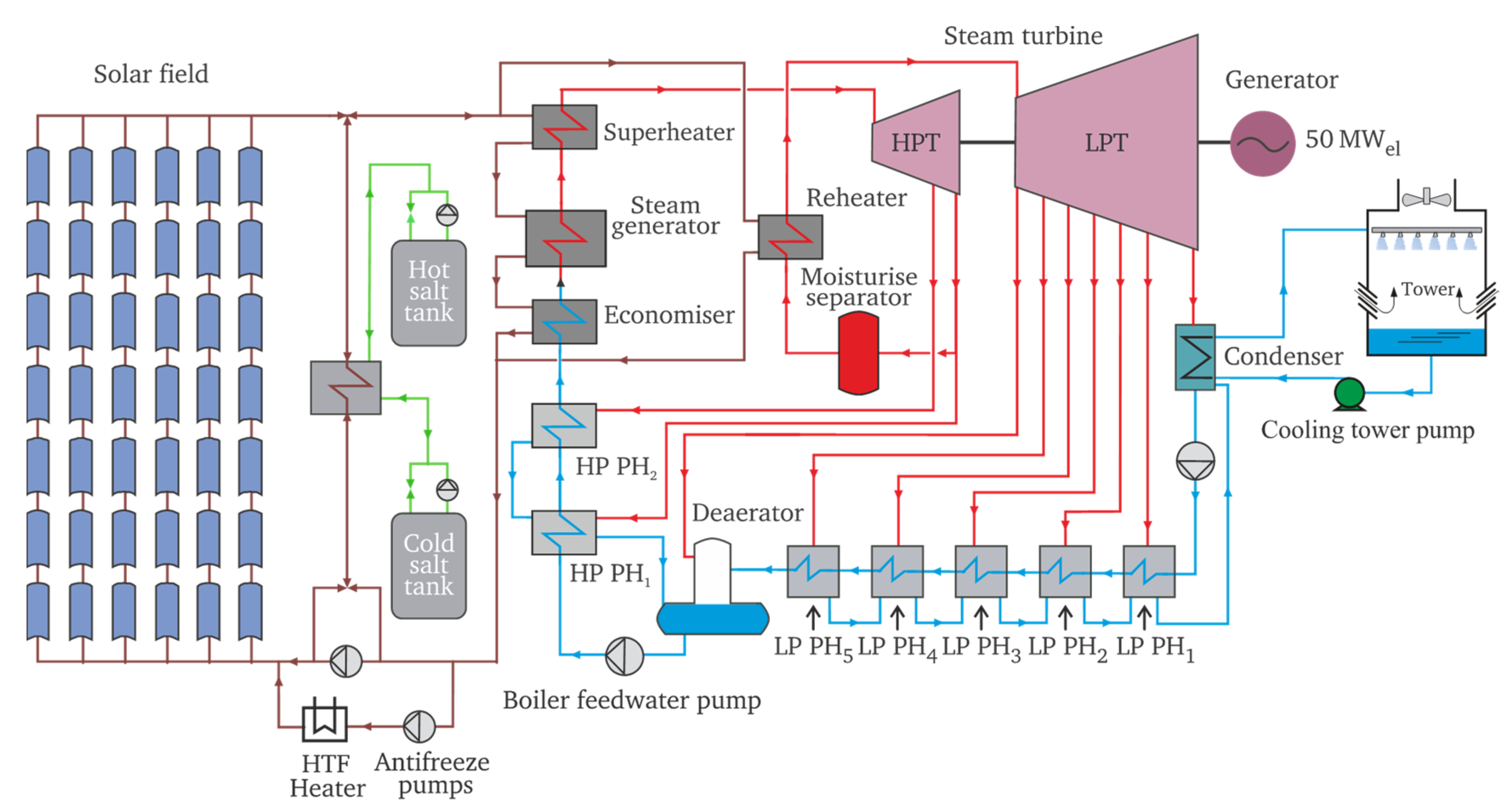
5. PTSPP Model Description

A schematic diagram of (PTSPP) “Andasol II” in Andalusia is demonstrated in Figure 2, including all parts (SF, TSS and PB).

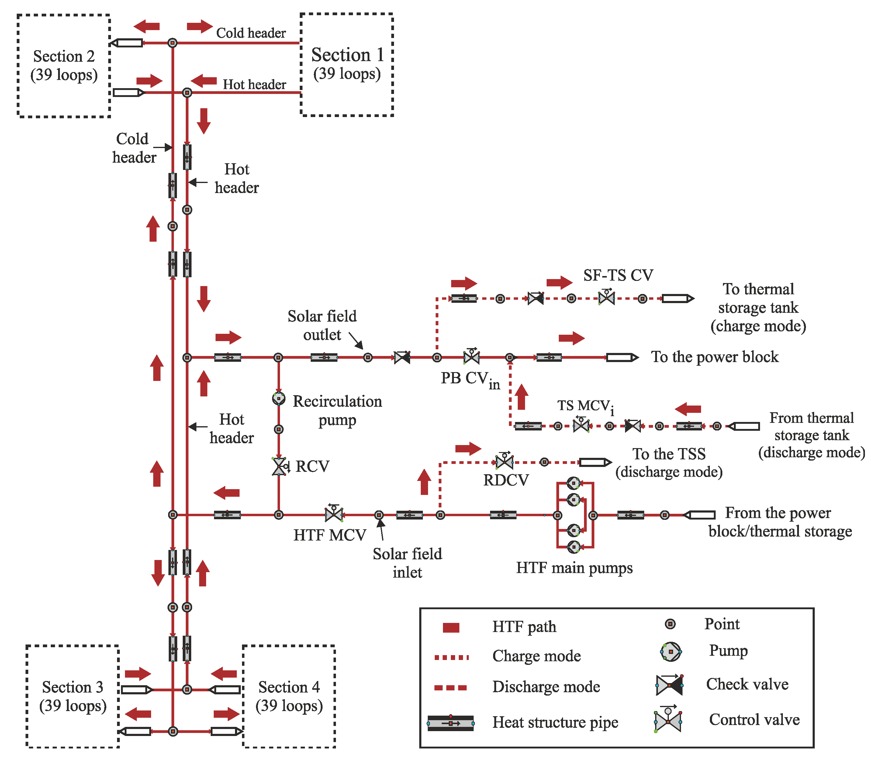
5.1. Solar Field (SF)

The solar field includes north and south sectors. Each sector includes two sections which contain 78 collector loops for both. The thermal oil coming from the economiser with 295 °C is pumped to the inlet of the solar field, as illustrated in Figure 3. Thereafter, the thermal oil is streamed to the north and the south sections through 312 collector rows. The HTF circulated through the collector loops is heated by solar radiation. The HTF in the north and the south loops will meet before the SF outlet. At the SF outlet, the hot HTF will be flow to either the power block, a storage system or to both.

The measured DNI represents the input into this model. Initially, the HTF mass flow rate is increased to 390 kg/s and is maintained until the designed inlet temperature (295 °C) is reached. In this process, each section of the SF accumulates a specific amount of thermal energy. After reaching the designated temperature at the entrance, the mass flow rate of the thermal oil and its temperature gradually increase until the maximum mass flow rate (1170 kg/s) is reached at the designated exit temperature (393 °C). Furthermore, the pressure losses for the power plant components are already included in this model.

In dynamic simulation it is very important to use the controllers to complete the simulation with high accuracy. Only the most important control circuits will be described briefly:

(1)

The SF-TS valve regulates the surplus thermal oil to the hot storage tank. This valve is opened when the HTF mass flow threshold value is 600 kg/s and the temperature is 393 °C.

(2)

The PB CVin adjusts the nominal value of HTF mass flow of 600 kg/s to the PB.

(3)

The DNI controller sets the real data of solar radiation measured in Spain to the HTF in four sections.

(4)

The HTF MCV valve at the SF inlet controls HTF temperature at the SF outlet. This valve performs two functions: First, it adjusts a mass flow of 390 kg/s after sunrise in the SF and remains at this value until the HTF temperature at the outlet of SF has been raised up to 295 °C due to the increase in DNI. Second, after achieving 295 °C of thermal oil temperature at the outlet of SF, the second function is enabled. This valve controls the temperature of HTF at the outlet of SF to obtain the design temperature at the SF exit (393 °C).

5.2. Thermal Storage System (TSS)

This system provides the stability in the production of electric power and high flexibility in operation. Two insulated tanks connected to each other by six heat exchangers are used to model the storage system in APROS. A series of heat pumps are installed beyond the storage tanks to pump the molten salt into the heat exchangers. The density and specific heat properties of the molten sodium and potassium nitrate salt mixture are known as a function of temperature.

In the charging phase (high solar radiation), the molten salt from the cold tank is heated by HTF up to approximately 386 °C and it is then sent to the hot salt tank. At this point it should be mentioned that there are losses between the HTF and the molten salt in the series of heat exchangers. That means that the temperature of the hot molten salt drops under the maximum HTF temperature of 393 °C, while the hot molten salt achieves a temperature of 386 °C. Consider that the maximum capacity of the TSS is approximately 1025 MW_th h.

In the discharging phase (evening or cloudy periods), the HTF is heated using hot molten salt. In this case, the TSS supplies the HTF’s nominal mass flow (600 kg/s) with a temperature of 377 °C in the night hours. This affects the steam generation capacity, while the nominal amount of steam generated during the day (55 kg/s) is not reached in the evening hours. When the heat exchange between molten salt and thermal oil has been completed, the cold molten salt with a temperature of 292 °C enters the cold tank.

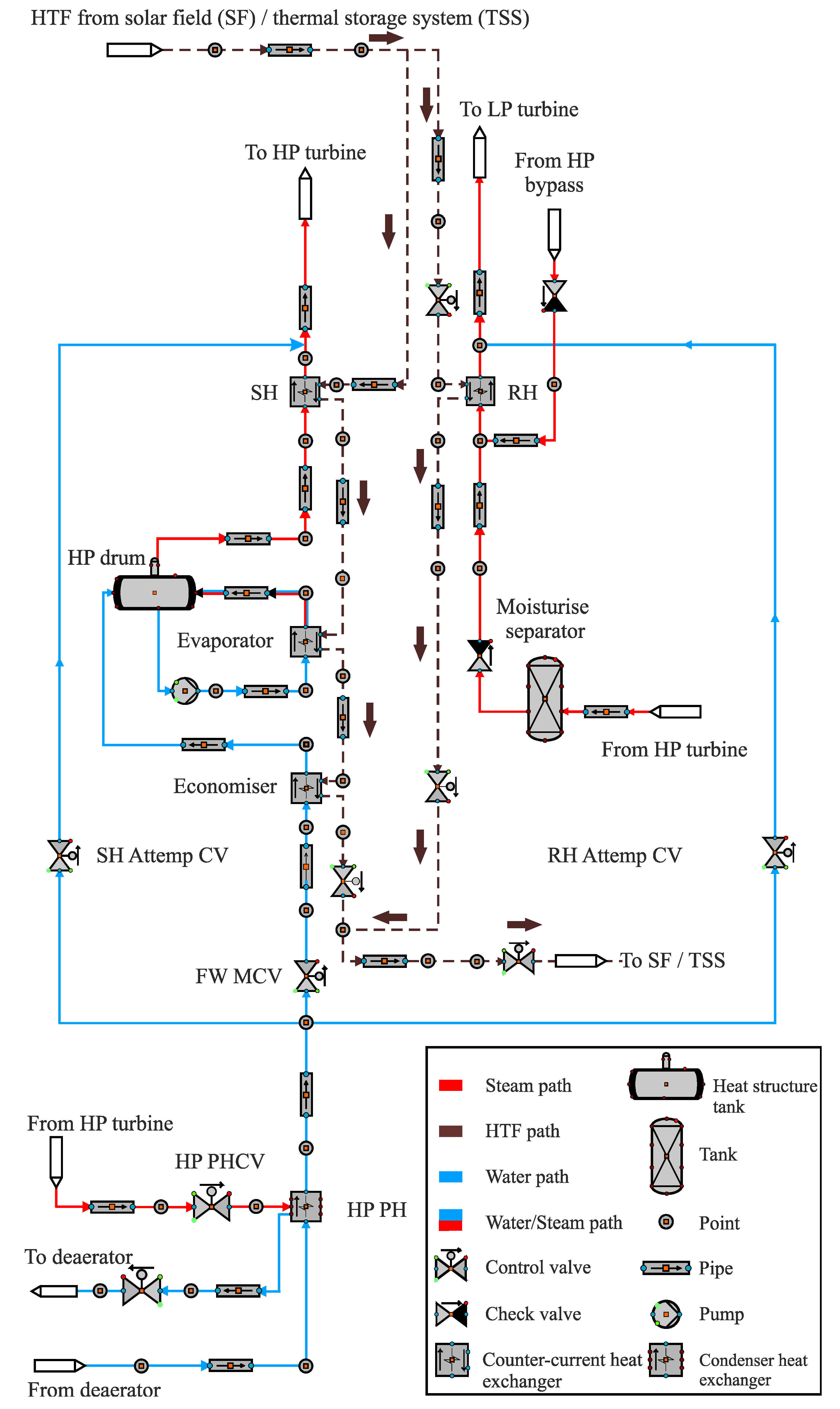
5.3. Power Block (PB)

The boiler in this power plant consists of a series of heat exchangers. Each line includes a superheater, evaporator, economiser and reheater. The steam–water path is designed based on two pressure sections, namely the main system pressure and reheat sections, as described in Figure 4.

The water coming from the condenser enters a low-pressure feedwater circuit. Thereafter, it passes through five low-pressure preheaters to raise the temperature from 35 °C to 165 °C at the outlet of LP PH₅ (low pressure preheater) using the steam extracted from the LP turbine. The water is then collected in the deaerator, which is considered a type of open water heater. It is then pumped to the HP preheaters before entering the steam generator. In the deaerator, the water is purged of oxygen by HP steam flowing from the HP turbine to avoid corrosion.

Both HP and LP preheaters work by the steam extracted from the turbine. These heat exchanger preheaters contain tube and shell sides where the extracted steam is condensed in the shell side while the water is heated in the tube side. Although the steam extracted from the turbine reduces the turbine power production, it also raises the feedwater temperature in the tubes, resulting in an improvement in the plant cycle efficiency.

The steam exits the economiser and streams into the HP feedwater tank. The level of the HP tank is regulated by the HP feedwater main control valve (FW MCV_HP). The circulation process between the evaporators and HP tank is carried out by the HP recirculation pump (HPRP) which generates saturated steam. Here, the HP tank works as a separator. While the water remains in the drum and mixes with water coming from the economisers, the saturated steam leaves the drum and enters to the HP superheaters, and here saturated steam absorbs additional heat from the thermal oil. Then, the HP superheated steam enters the HP turbine part. The steam temperature is kept from increasing above 384 °C at the turbine inlet by the HP attemperator, which is placed at the superheater outlet. The HP attemperator is supplied the feedwater by the HP feedwater pump.

The pressure and temperature of steam entering the steam turbine are 106 bar and 384 °C, respectively. On the one hand, part of the steam is extracted to the high-pressure preheater (HP PH), while on the other hand, part of the steam is streamed to the reheaters in order to reheat the steam up to 383 °C. Thereafter, the reheated steam enters the LP turbine with a pressure of 19.4 bar. At the outlet of the LP turbine, the steam flows into the condenser. After condensing the steam, the water is pumped using condenser pumps to the LP preheaters and then the cycle will continue in the power plant again.

Table 1. Technical data of the real power plant.

Andasol II	Units	SF	TSS	HP Turbine	RH/LP Turbine
Working Fluid		HTF (Thermal Oil)	HTF (Thermal Oil)	Steam
Conditions at the inlet	(bar)	P = 31.3	P = 17.5	P = 104	P = 19.4
	(°C)	T = 295	T = 393	T = 384	T = 383
	(kg/s)	$\dot{m}$ = 1100	$\dot{m}$= 500	$\dot{m}$= 54	$\dot{m}$= 44.3
Conditions at the outlet	(bar)	P = 18.2	P = 12	P = 20.5	P = 0.05
	(°C)	T =393	T = 293	T = 215	T = 30
	(kg/s)	$\dot{m}$ = 1100	$\dot{m}$= 500	$\dot{m}$= 47.7	$\dot{m}$= 33.7

shows the properties of steam and HTF obtained from the Andasol II plant at the nominal load.

To regulate the operating process of the power plant, it is essential to have control circuits. Here, the controllers for the LP/HP preheater level, the SH and RH attemperator, the drum level, the economiser water bypass and the steam bypass control circuits are implemented in this model.

• Undesired steam is bypassed by HP and LP bypass controllers to the reheater and condenser before entering the HP and LP turbine, respectively. These controllers are used in the shutdown and start-up processes as well as for the steam turbine trip of any load.
• The attemperators (SH Attemp CV and RH Attemp CV) adjust the steam temperature to (384 °C) at the turbine inlet. This cooling process is implemented by injecting some of the water from the boiler water pump to the attemperators.
• In order to achieve the stability of flow in the evaporator, a small amount of water transferred from the economiser inlet is bypassed into the inlet of the drum. Here, the water temperature at the outlet of the last economiser is kept under the boiling temperature with a sub-cooling temperature of 5 °C by the economiser water bypass controller.
• The drum-level control valve adjusts the mass flow flowing into the drum in order to avoid instability caused by fluctuations in the water level in the tank.
• Seven control valves of LP/HP preheater level keep the water level of preheaters at certain values due to changes caused by condensation of extracted steam on the shell side.

6. Results

The suggested model was verified against the experimental data obtained from Andasol II in [22]. The simulated results in this section were compared with the experimental data on 2 July 2010 to generalize the model validity and test the effectiveness of the adopted operating strategy. The power plant operation strategy is dynamically controlled by many control circuits during the day regardless of DNI oscillations. The strategy of the developed model was compared versus the strategy of the real power plant through the measured data on this day. This day in July was cloudy. The simulated predictions for the dynamic HTF behaviour in the SF, the TSS and the PB are displayed. In addition, the model results of the dynamic behaviour of steam in the power block are discussed.

6.1. Heat Transfer Fluid Behaviour

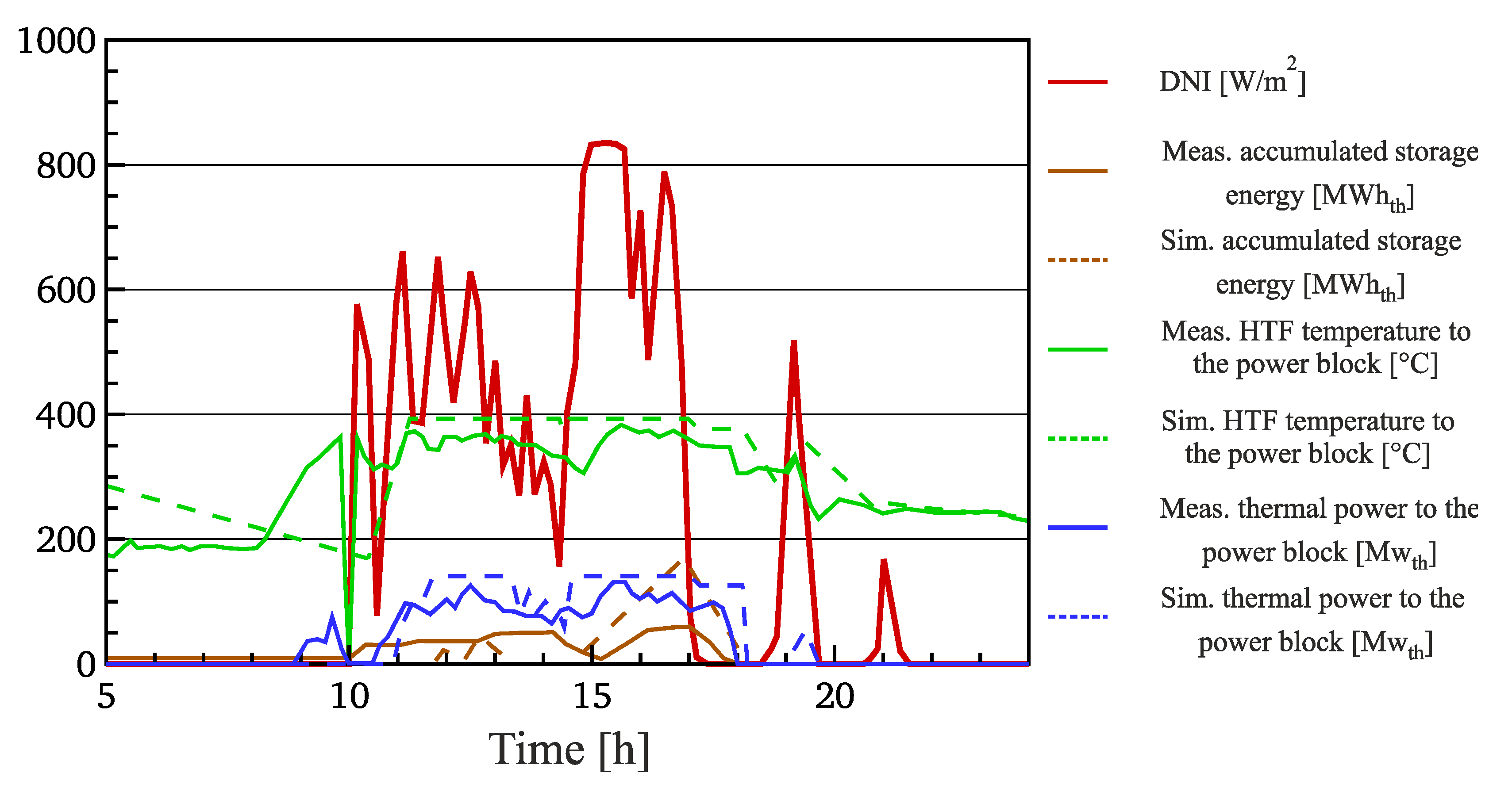
The simulation results and experimental data are compared on 2 July 2010, including (DNI), the HTF temperature at the exit of SF, the thermal energy transmitted to the PB and the thermal stored energy accumulated in the TSS.

In Figure 5, DNI data were measured in several weather stations on a selected day at the location of Andasol II. The average values of this data were used as inputs to the power plant model for the chosen day.

After the outlet of SF, the simulated thermal oil temperature on 2 July 2010 displayed a good match with the measurements, as illustrated in Figure 5. At t = 9:59, a technical fault occurred, causing a drop in the measured temperature of HTF to 0 °C. The warm-up periods in the SF include two phases. The first phase begins at sunrise. As a consequence, the temperature of HTF raises from 170 °C to the designated temperature at the inlet of the SF (295 °C).

In the second of the warm-up phase, the simulated temperature of thermal oil continues to rise until the designated temperature of the SF outlet (393 °C) is at t = 11:13. Additional heating of the HTF temperature is avoided by controlling the HTF flow through the SF to maintain the temperature of HTF at the designated outlet temperature (393 °C). Between t = 11:13 and t = 14:18, the temperature is kept stable at 393 °C despite severely fluctuating DNI values. After t = 14:18, the HTF temperature drops and reaches 375 °C because of the absence of stored energy and low DNI. At t = 14:30, the temperature of thermal oil increases to the designated outlet temperature. Thereafter, the temperature of thermal oil remains constant until t = 16:59, and here the HTF temperature decreases to 377 °C at t = 17:10 because the power plant operates in thermal storage mode. At t = 18:04, the simulated HTF temperature decreases from 377 °C to 287 °C at t = 18:49 because of the absence of stored energy, and DNI is completely absent due to dense clouds. After t = 18:49, the power plant continues operating only with the thermal storage until the end of the day. After the clouds clear, the thermal oil temperature rises again to 355 °C at t = 19:22. Afterwards it decreases to 250 °C because of heavily cloudy skies. At t = 21:00, the temperature increases again to 293 °C because of the removal of clouds. Thereafter, the temperature drops because of the sunset.

Thermal power transferred to the PB is calculated based on the HTF mass flow at the inlet of PB and the variation between the thermal oil temperature at the inlet and the outlet of SF. In the actual power plant between t = 8:49 and t = 9:59, thermal power is generated even though there is no DNI, and storage power is exhausted. This indicates that the power plant was running on the fuel system during this period. Hence, this difference affects the production of electricity, which is dependent on the thermal energy behaviour. At t = 10:53 thermal power is produced based on DNI and reaches and reaches 101 MW_th at t = 11:17, as shown in Figure 5. After that, the transferred thermal power drops to 99 MW_th and shows a decline of solar radiation suddenly. At t = 11:42, the maximum value of the transferred thermal power (140.72 MW_th) is achieved.

Then, this continues constantly until t = 13:18. This is due to the presence of solar radiation and adequate thermal storage. After t = 13:20, the thermal power drops to 80 MW_th at t = 13:30 because the PB only works with the SF mode. From t = 13:30 to t = 14:24, the experimental and simulated thermal power oscillates because of changes in the total HTF mass flow to keep the designated outlet temperature.

Thereafter, the thermal energy transferred to the PB rises again to the set value and maintains this value after t = 14:33 because of the increase in DNI. The transmitted thermal power reduces to 125.75 MW_th as a result of decreasing the design outlet temperature to around 377 °C. After t = 18:04, the thermal power reduces to zero and remains constant because of the depletion of stored energy. After the demise of the clouds, the thermal power reaches 54 MW_th at t = 19:24 and then reduces to the zero value as a result of the DNI reduction. Although the DNI was high again after heavily cloudy periods, the thermal power transferred to the PB remained at a zero value until sunset. This is because the designated temperature at the inlet (295 °C) was not achieved as the solar radiation was not enough.

In Figure 5, the experimental stored energy accumulated in the TSS shows a good match with simulated energy. At t = 11:42, a set value of the transferred thermal power to the PB is achieved. As a result, the excess heat is either transferred to the hot salt tank or dissipated when the hot salt tank is completely filled, i.e., reached 1025 MW_th h. The thermal oil (HTF) enters and exits the TSS at temperatures of 393 °C and 293 °C, respectively. In the storage discharge period, the temperature of thermal oil is set to be 293 °C and 377 °C at the inlet and outlet of TSS, respectively. From t = 11:43 to t = 13:22, the thermal power transferred to the PB is collected from the SF and the TSS. At t = 13:22, the TSS is exhausted and remains empty until t = 14:32. At t = 16:52, the thermal storage capacity reaches 170 MW_th h. After that, the discharge period lasts about 1.35 h until the TSS is fully exhausted. From t = 18:12 to sunset, all the heat absorbed in the SF is transmitted to the PB to achieve the specified values of thermal oil mass flow and temperature of 600 kg/s and 393 °C, respectively. Therefore, no excess heat is found in TSS because of heavily cloudy periods. On the other hand, the measured stored energy is sent to the thermal storage system at t = 9:59 instead of the power block, then this process continues until t = 10:27. From t = 10:27 to t = 14:09, the collected heat is sent together to the PB and to the TSS despite nominal thermal power still not being achieved. Thereafter, the measured stored energy is decreased to replenish the lost heat due to the cloud cover. The measured storage energy rises again at t = 15:09 and continues increasing until t = 16:59, accompanied by oscillations in the measured transmitted thermal power. The accumulated thermal storage then drops to (0 MW_th h) at t = 17:59 due to the real power plant operating in storage mode.

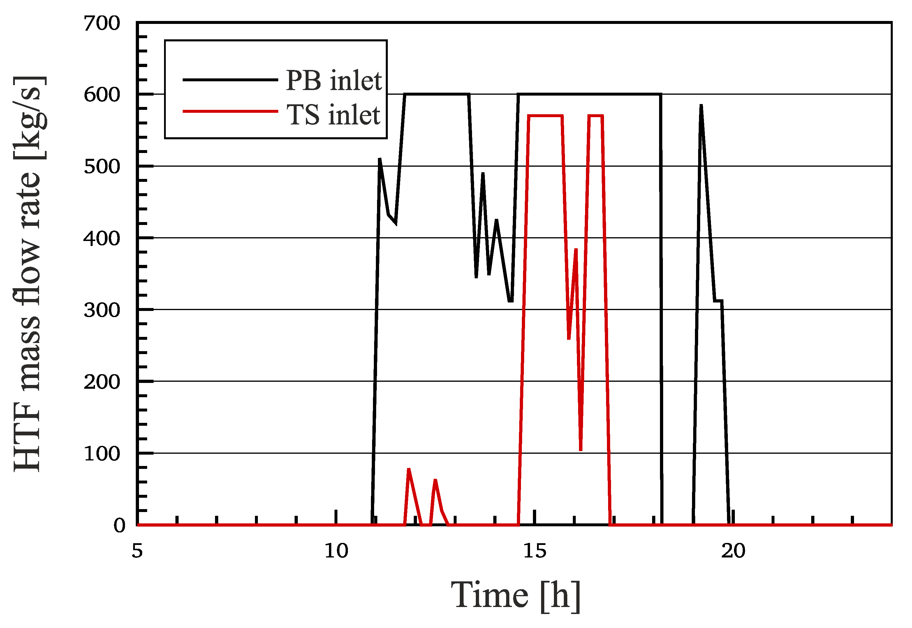
Figure 6 shows the simulated HTF mass flow to the TSS and to the PB on 2 July 2010. The operating principle that was adopted to obtain these results shown in Figure 6 ensures the nominal HTF mass flow (600 kg/s). The surplus of thermal energy is transferred to the TSS, and this energy is also used to compensate for the shortfall in thermal power.

Finally, the comparison of simulation predictions and experimental data displays a good agreement until t = 17:59 on 2 July. This does not prevent some differences between the simulation and experimental after t = 17:59, as previously demonstrated. The discrepancies between the simulation and experimental are explained as follows: The operational steps were taken in the Andasol II plant to transfer the thermal power to TSS instead of transferring the power to the PB.

6.2. Steam Behaviour

In this section, the steam parameters (steam mass flow and steam pressure) in different points in the Andasoll II are measured for the specified day at the nominal load. The dynamic behaviour of these parameters in the PB will be explained below.

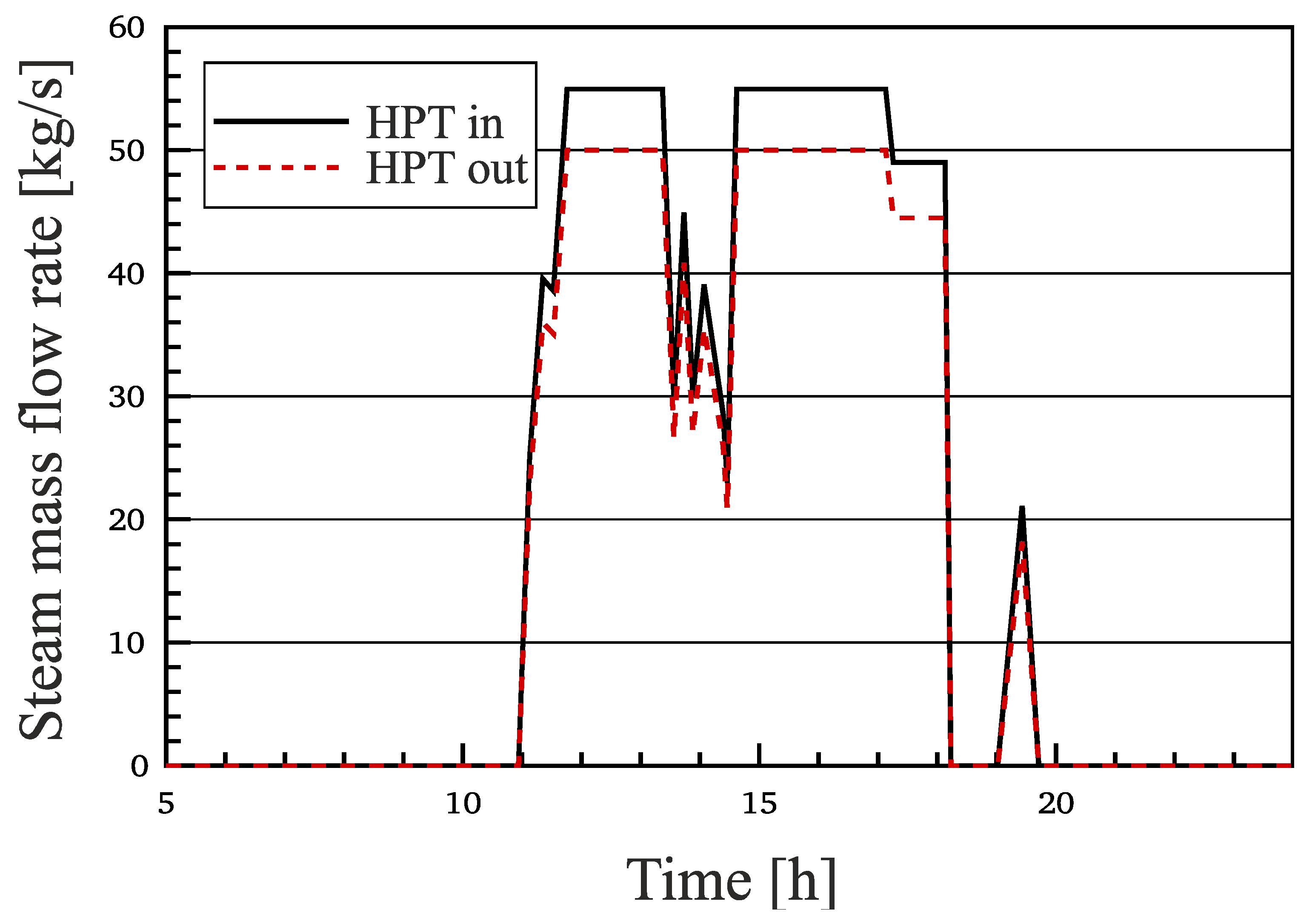
The HP cycle is implemented between the exit of the HP feedwater pumps (HP FP) and the outlet of the last superheater. The dynamic behaviour of the water/steam path is presented by the following figures.

The model results of the mass flow of steam at the inlet and outlet of the HP turbine are demonstrated in Figure 7 for the selected day.

At t = 10:50, the mass flow of steam begins to increase until its specified value reaches about 55 kg/s at t = 11:40. The HP steam mass flow remains at this value until t = 13:20. Then, the mass flow of steam drops to 25 kg/s at t = 13:32 because of the lack of stored energy and the oscillations of HTF mass flow due to clouds. Here, the PB is only operated in SF mode. Between t = 14:33 and t = 17:06, the steam mass flow remains constant (55 kg/s). Between t = 17:14 and t = 18:06, the steam mass flow reduces down to 44.5 kg/s since the power plant operates only in storage mode. Then it drops to zero at t = 18:12 when the storage energy is exhausted. The steam mass flow increases at t = 19:54 again to 21 kg/s due to higher solar radiation. Thereafter, it drops to zero and continues at this value until sunrise the next day.

The steam mass flow at the outlet of the HP turbine displays similar behaviour to that of the steam mass flow at the inlet of the HP turbine for the chosen day, as illustrated in Figure 7. The difference in the steam mass flow between the HPT inlet and outlet is due to the steam extractions that are connected with the HP preheaters.

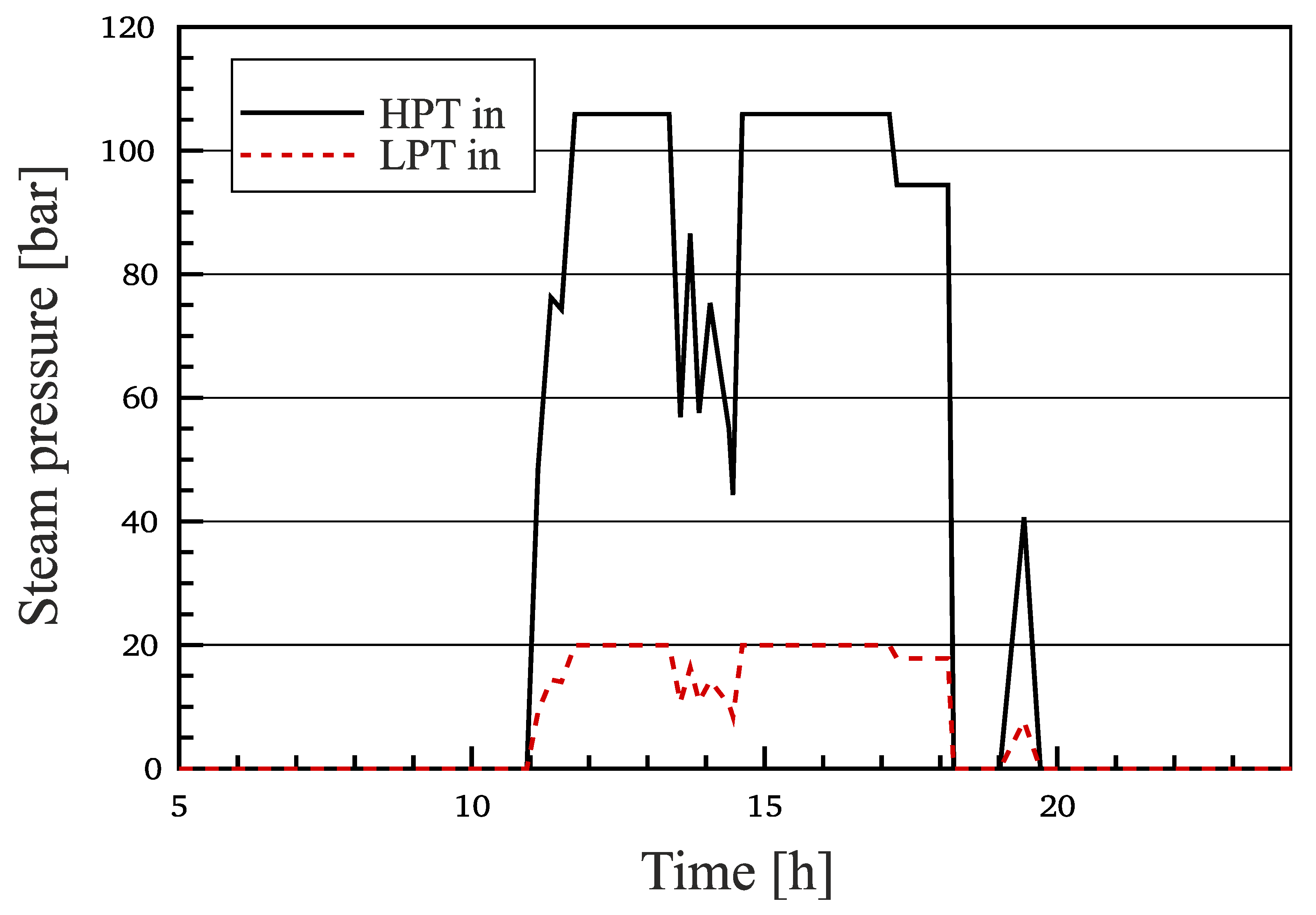
Figure 8 displays the dynamic behaviour of the steam pressure at the inlet of the HP turbine. The pressure of steam rises to a set value of 106 bars due to the generation of steam in the PB. After that, it continues at this value in the period between t = 11:44 and t = 13:20. From t = 13:20; the steam pressure decreases to 57 bars. Then, it fluctuates until t = 14:26. The steam pressure rises again to its set value at t = 14:35 and then it continues constant until t = 17:06. The steam pressure decreases to 94.42 bars and is kept constant for one hour, then decreased to (0 bars) at t = 18:12. At t = 18:59, the steam pressure rises again to 40.64 bars due to higher DNI. Subsequently, the vapour pressure drops to zero at t = 19:41 and remains to sunset because there is no storage energy and there is no solar radiation due to the clouds. The steam pressure of the LP turbine behaves the same as the steam pressure of the HP turbine.

7. Conclusions

A detailed dynamic model of a parabolic trough solar power plant (Andasol II) was carried out by (APROS) Software with required control circuits. The model was implemented using the realistic details obtained from a real plant. A comparison between the simulations results and experimental data from “Andasol II” was applied.

It is obvious that the model results agree well with the experimental data in some periods ranging between t = 10:28–17:59 for the selected day. Conversely, several discrepancies can be observed between the simulated results and the experimental data for the rest of the day. This is due to the fact that, on the one hand, the operator’s decision during overcast periods was different from that performed in the model, and on the other hand the power plant was operated based on the fossil fuel system during some periods, as well as a technical fault in the measured data that occurred around t = 9:53. Note that the operator’s decisions can also be included by the APROS model, but that will be at the expense of the dynamic behaviour of simulation, i.e., the simulation will be conducted as a steady-state model. However, the operation strategy applied in the dynamic model during cloudy day improves the electrical power production compared to the operator’s decisions that were implemented in the real power plant. About 28% (about 2.7–3.1 h) of electric power generation was increased during the discharge and charge phases of the chosen days.

This model is important for understanding the operation strategy of the power plant and possibly for other plants in other operating conditions to benefit from it.