Feature-Based Multi-Class Classification and Novelty Detection for Fault Diagnosis of Industrial Machinery

Abstract

Given the strategic role that maintenance assumes in achieving profitability and competitiveness, many industries are dedicating many efforts and resources to improve their maintenance approaches. The concept of the Smart Factory and the possibility of highly connected plants enable the collection of massive data that allow equipment to be monitored continuously and real-time feedback on their health status. The main issue met by industries is the lack of data corresponding to faulty conditions, due to environmental and safety issues that failed machinery might cause, besides the production loss and product quality issues. In this paper, a complete and easy-to-implement procedure for streaming fault diagnosis and novelty detection, using different Machine Learning techniques, is applied to an industrial machinery sub-system. The paper aims to offer useful guidelines to practitioners to choose the best solution for their systems, including a model hyperparameter optimization technique that supports the choice of the best model. Results indicate that the methodology is easy, fast, and accurate. Few training data guarantee a high accuracy and a high generalization ability of the classification models, while the integration of a classifier and an anomaly detector reduces the number of false alarms and the computational time.

1. Introduction

Fault Diagnosis (FD) has been extensively studied in recent years, especially data-driven approaches applied to condition monitoring data. In this approach, fault diagnosis consists of collecting sensor data from machinery and finding the relationships between their values and specific machine’s faults. In a recent review on intelligent fault diagnosis [1], the authors analyzed more than four hundred articles. They showed that the research focus has moved from traditional signal processing and Machine Learning (ML) models, mostly adopted until 2010, to Deep Learning (DL) and Transfer Learning (TL). The diagnosis process using traditional approaches includes data collection, feature extraction and selection, and health state recognition [2]. The critical aspect of this approach is the extraction and selection of representative features, which require expert knowledge and time-consuming data processing. DL-based fault diagnosis approaches solve this issue, as the deep network structures automatically learn high-level and non-linear representations of input data [3]. However, both ML and DL approaches require massive, labeled data to make the diagnosis system accurate and robust. TL offers a promising solution that uses the knowledge acquired from a source domain, for which sufficient labeled data were available, for improving the prediction performance of a target domain, where massive labeled data are not available [4]. Hence, TL represents a powerful tool, especially for complex systems or machinery working under different operating and environmental conditions. However, it relies on the assumption that there are sufficient labeled samples for building a good classifier in the source domain.

From the industrial perspective, the availability of a large amount of data collected during nominal and faulty operating conditions is a critical aspect [5]. In particular, while it is easy to obtain data in nominal conditions, data in faulty conditions are hard to obtain given the loss of productivity and the quality, environmental, and safety issues arising from machinery working in faulty conditions [6]. Moreover, not all fault modes are known, and new operating conditions can occur during machine life [7]. In some cases, a physical model of the monitored system can be built to generate off-line datasets required by a classifier [8]. However, plant-models require investments whose return is hard to estimate. For this reason, especially for complex systems such as automatic machinery, no model exists to generate additional data [9]. As a result, TL-based fault diagnosis systems are not viable solutions in industries yet; on the other hand, traditional ML-based fault diagnosis and DL-based fault diagnosis should be built, considering the possibility to expand their knowledge during machine functioning. In other words, offline and batch fault diagnosis systems should be integrated with online and streaming models to recognize known conditions and detect unknown behaviors [10].

The task of detecting new data samples that an ML model was not previously aware of is called novelty detection [11]. Novelty Detection (ND) is traditionally considered a one-class classification problem, in which only one class, i.e., the nominal class, is known. Hence, it usually requires a dataset including many data samples belonging to the same class. Then, a decision model is learned based on labeled examples during the training phase, while a novelty detection algorithm is applied to streaming data to find the degree of novelty or similarity of current data samples in respect to the learned class [12]. Unlike anomaly detection and outlier detection, novelty detection aims to find a set of points not explained from the diagnosis model, instead of one single point differing from the nominal or known data [13]. In addition, novelty detection is also included in multi-class systems, where there are two or more nominal classes exist, and a condition is considered novel if it differs from all of the known classes [14]. In other words, the problem becomes recognizing novelties and, at the same time, classifying the known instances into two or more diverse classes. The first relevant papers on this topic were published in early 2000. In [15], the authors highlighted how threshold-based classifiers might be appropriate for condition monitoring and fault diagnosis systems, as they allow us to interpret an unknown fault when none of the classifier output exceeds the defined threshold. In [16], an unsupervised neural network named Self-Organizing Feature Map (SOFM) is first used to detect novelties in rotary machinery; then, a supervised and probabilistic Radial Basis Function (RBF) classifies the detected novelties in one of the known classes. Carino et al. [17] proposed an incremental learning-based methodology for novelty detection and fault diagnosis of an industrial electromechanical system. It consists of an ensemble one-class classifier for novelty detection and an evolving and unsupervised classifier for fault diagnosis. More recently, deep learning models, such as autoencoders and Long Short-Term Memory (LSTM) networks [18,19,20], are used to detect novelties and simultaneously classify known nominal and faulty conditions. Another approach to novelty detection sees novelty as a concept, an abstraction of cohesive and representative examples, that introduces characteristics different from known concepts [21]. In this sense, several clustering algorithms for novelty detection in data streams have been proposed, such as OnLine Novelty Detection and Drift Detection Algorithm (OLINDDA) [21], Higia [22], and MINAS (MultIclass learNing Algorithm for data Streams) [12]. The idea behind these algorithms is to learn a decision model based on labeled data during the offline training phase; then, during the online phase, novelty patterns are recognized as unknown sets, or micro-clusters, made of examples that the model does not explain. Even in these cases, the offline decision model can represent different classes.

In this paper, novelty detection and fault diagnosis are conducted to detect the occurrence of anomalous behavior that may correspond either to a known or novel condition in an automatic packaging machine. In particular, novelty detection is performed through an anomaly detection algorithm and a classification model. The anomaly detector is trained on nominal samples. Its role is to identify samples that deviate from the nominal behavior. Then, if two subsequent anomalies are detected, they input a pre-trained probabilistic classification model, which computes a probability class membership for each class. If the maximum class probability is lower than a certain threshold, the detected anomalies are considered novel, and an alarm is triggered. In other words, thanks to the classifier that is trained on the samples corresponding to the known faults, it is possible to determine the kind of the anomaly (one of the known faults). On the contrary, the novel behavior is detected when the same classifier does not classify a sample accurately (the maximum class probability is lower than the fixed threshold). Contrary to existing approaches, in which the pre-trained classifier always makes an inference on the data to support the novelty detection, in this paper, the inference by pre-trained models on streaming data is only made when two consecutive anomalies are detected. Therefore, the computational time is reduced as the inference is only made on detected anomalies. In addition, when a novel condition is detected, the classifier for fault diagnosis has to be re-trained to include the novel condition. In some applications, it is a desirable, automatic re-training. The anomaly detector before the classification model can keep the data that correspond to the nominal condition separate. Therefore, the classification model can be re-trained using only the data already available and corresponding to the nominal condition, and the data collected during known and novel fault conditions. This represents an advantage in case of limited storage memory and computational power. Additionally, keeping the number of nominal samples included in the dataset used for re-training the classification model low may help solve the issue of unbalanced dataset, which is a typical issue of fault diagnosis applications. Finally, the false alarm rate can be reduced, as the subsequent classifier might classify the detected anomalies as nominal.

The main contribution of the present study is the formulation of a complete and easy-to-implement procedure for streaming fault diagnosis and novelty detection and its application to an industrial machinery sub-system, for which a large amount of labeled data and a limited amount of faulty data are available. In particular, this paper uses different ML techniques for fault diagnosis and anomaly detection and evaluates them in terms of the ability to provide, in their whole, indications about the occurrence of novel behaviors. Finally, the paper aims to offer useful guidelines to practitioners to choose the best solution for their systems, including a model hyperparameter optimization technique that supports the choice of the best model.

The remaining of the paper is organized as follows. Section 2 provides the theoretical background of Machine Learning-based fault diagnosis, novelty detection, and feature extraction and selection models. Moreover, the framework of the proposed solution and the models adopted in this study are described. Section 3 describes the analyzed system and the data collected for validating the methodology. In addition, it shows the results of the application of the methodology to this system. Finally, Section 4 concludes the paper with final remarks and future research.

2. Materials and Methods

Fault diagnosis is a typical pattern recognition problem that can be solved through Machine Learning models for classification. Classification is a supervised learning task that requires a complete dataset including both predictors and the associated target class for each observation. In fault diagnosis, the predictors correspond to the features that are extracted from raw signals using signal analysis techniques, and the target class indicates the system’s conditions, such as healthy, fault, or the type of fault. The classifier’s task is to search for rules representing the relationship between features and faults [23].

Classification is usually performed in two steps, named training and testing. First, the whole dataset is divided into two subsets, named training set and testing set. The training set is used to learn the relationships between the features and the classes, and then a classifier algorithm is chosen that can apply these rules successfully to the observations in the testing set [24]. Finally, the actual class is compared with the class predicted by the classifier to assess its prediction accuracy. The selection of the classification algorithm is a critical aspect of the classification process. There are no precise rules for choosing a specific classifier, and there is no classification algorithm that works best for every problem. Each case requires comparing different classifiers to choose the most suitable model for the case under analysis. In general, a good classifier should have low complexity and high generalizability. A low complexity model can rarely fit the data in the training set optimally, resulting in a high error in both training and testing data. This problem is also called underfitting. A more complex model can be chosen to fit the data better and achieve a lower training error. However, increasing the complexity means reducing the model’s generalization ability, which is demonstrated by a higher prediction error on the test set. This problem is also known as overfitting. Hence, a good classification model should find the optimal trade-off between the complexity and the generalization ability, also named the bias–variance trade-off [25]. A solution to estimate the training and testing errors and evaluate a classifier is to apply the k-fold cross-validation. According to this technique, the whole dataset is divided into $k$ non-overlapping sets, and the training-test cycle is repeated $k$ times. One of the $k$ sets is held for testing at each iteration, while training is performed on the remaining $k-1$ sets [26]. In this way, $k$ different prediction accuracy values are obtained, and the final accuracy of the model can be obtained by averaging the $k$ values. Classifiers have two kinds of parameters, as do all Machine Learning models, named ordinary parameters and hyper-parameters [27]. The learning process in the training phase corresponds to the learning of ordinary parameters. On the contrary, the hyper-parameters are set before training and can either be set manually by the user or optimized through automatic selection methods. Hyper-parameters optimization (HPO) has several advantages, including reducing manual effort, improving model accuracy, and support model selection [28].

Fault diagnosis is usually performed in one step, as described in this section. However, by definition, diagnostics also include a previous phase named fault detection, which aims to assess if a fault has occurred [29]. This step is beneficial when novel behaviors need to be detected. In these cases, fault detection is usually faced through anomaly detection models, which aim to discover patterns in data that do not conform to expected behaviors [30]. Hence, anomaly detection is mainly devoted to recognizing the observations in a set of data that are far away from the majority of nominal data and thus are supposed to contaminate the available dataset [13]. On the contrary, novelty detection is a more suitable task when a novel fault behavior must be recognized. The goal of novelty detection is to recognize novel conditions that can evolve during machine running [11]. It is a Machine Learning problem that aims to identify new concepts in unlabeled data [31]. Novelty detection is often faced as a one-class classification problem, in which classification models are trained only on the nominal class [32]. In these cases, the training procedure is the same as the multi-class classification. In other cases, unsupervised learning-based models, such as clustering models, are used when novelties need to be recognized in streaming data [22,33]. Clustering approaches can be based on distance measures or density measures. The idea is that nominal samples are very close to each other in the feature space, i.e., nominal clusters are very dense, while anomalies or novelties are far from the nominal cluster and very sparse [34].

In this paper, novelty detection is performed through an anomaly detector and a classifier. Hence, basic concepts of the learning paradigm briefly described at the beginning of the present section for fault detection and fault diagnosis represent the basis for the novelty detection approach presented in this paper.

2.1. The Methodology

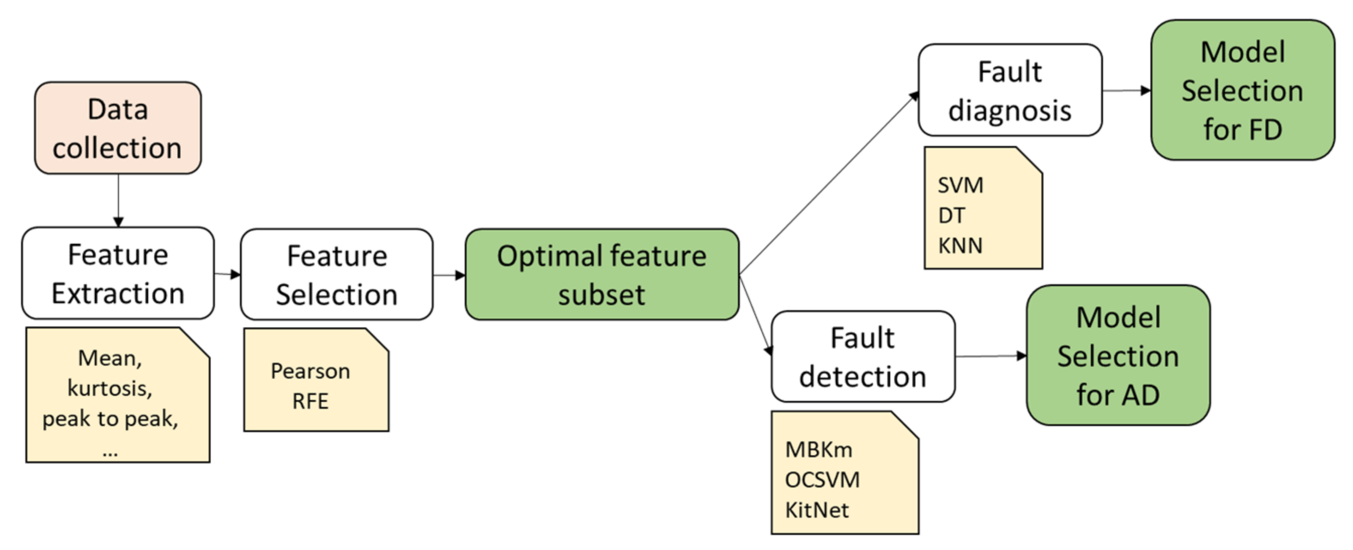
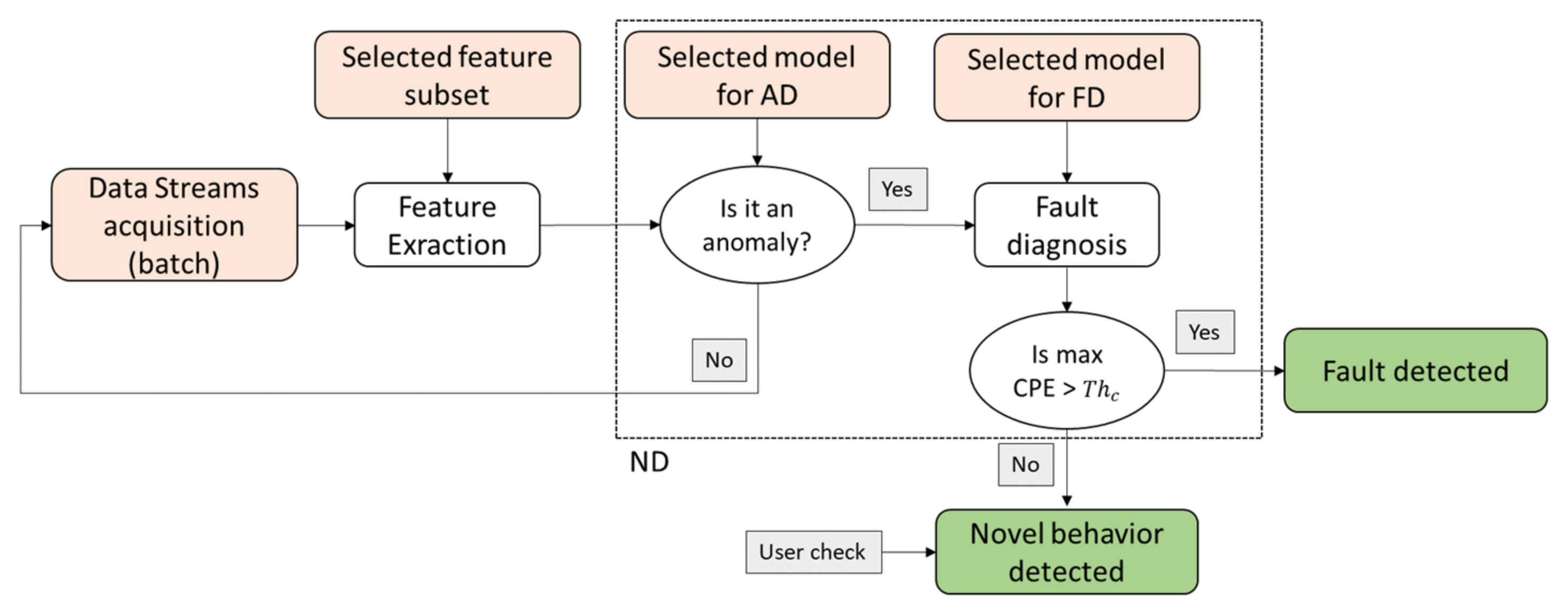
The proposed methodology consists of two parts, i.e., offline training and online condition monitoring, depicted in Figure 1 and Figure 2, respectively. The offline training includes the typical diagnostic process steps, i.e., data collection, feature extraction, feature selection, model selection, and model training for fault classification [2]. This phase aims to find the best feature subset and the best models for fault detection and diagnosis (novelty detection). The online condition monitoring aims to assess the current condition of the monitored system. Hence, based on the output of the training phase (green squares in Figure 1), it evaluates if the extracted feature vector from a signal segment of a defined length can be classified into the nominal class, into one of the known faults, or corresponds to a novel behavior.

The methodology was coded in Python using several libraries, e.g., Numpy, Pandas, SciPy, and Sci-Kit learn. For models training and testing, an Intel^® Core^TM i7- CPU @ 2.8 GHz and 16.0 GB RAM workstation has been used.

The following subsections describe each part of the methodology.

2.1.1. Data Collection: The Industrial Case

Data collection consists of collecting data able to reveal the health condition of a component/system. These data can be vibrations, acoustic emissions, currents, temperatures, and others, and the choice depends on the kind of system/component and the already available sensors [35]. The data collected for fault diagnosis should include the nominal and all possible fault conditions. However, data collection in fault conditions is challenging in industrial contexts due to safety, time, and economic issues. This difficulty is particularly evident for machine producers, who only can collect data during quality tests [36]. In these cases, as in the present case study, faults are manually induced on the system, and signals are collected for few minutes in each condition. For this reason, the system is assumed to either function correctly or not. In addition, these faults do not cause the system’s breakdown but introduce unacceptable qualitative issues on the product.

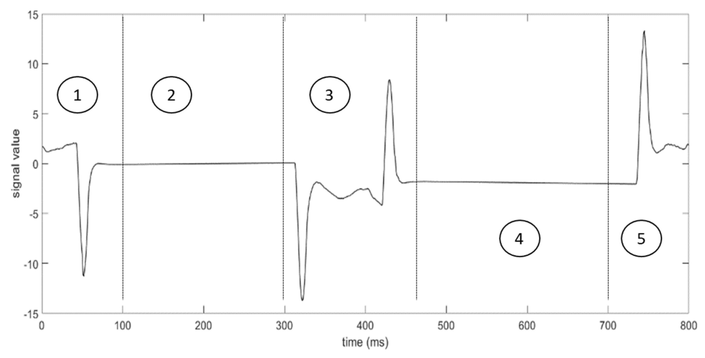
In this paper, a case of an automatic machinery of a manufacturer operating in the pharmaceutical sector is considered. The machine under analysis is a packaging line made of two parts connected by an automatic robot. The first section is a thermoforming machine that realizes the products in different materials; the second section is a cartooning machine, which packs the product into the carton. The machine can produce up to 320 products per minute and more than 260 cases per minute. This paper analyzes failures and malfunctions of the sealing group, which is placed in the first section and is responsible for sealing the two parts of the product. The group includes two tables, in which the film flows horizontally and continuously, allowing the sealing at a low temperature. Each sealing cycle consists of five steps: (1) the top table goes up, (2) the tables close, (3) the cover is sealed to the base, (4) the tables open, and (5) the parts return to the initial position. Figure 3 depicts the trend of the measured signal during a sealing cycle, which is divided into 5 areas, corresponding to the steps of the process. Each cycle lasts 800 milliseconds, and the sampling frequency of the sensor is 1000 Hz.

Table 1. Available dataset.

Dateset	Condition	Number of Cycles
D1	Nominal 1	360
D2	Fault 1	240
D3	Fault 2	200
D4	Restored 1	70
D5	Fault 3	100
D6	Restored 2	110
D7	Nominal 2	108
D8	Nominal 3	48
D9	Fault 1	93
D10	Fault 3	90

summarizes the test performed on the system with the corresponding number of cycles included in the test. In total, four conditions are available, i.e., nominal, fault 1, fault 2, and fault 3. The condition “restored” is assumed to be equal to the nominal one. Hence, almost 50% of the available dataset corresponds to the nominal condition, while the remaining part includes three different fault conditions.

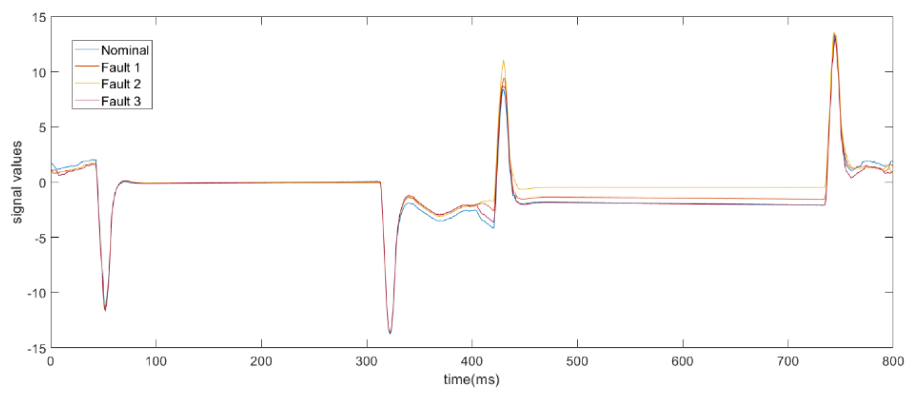
In Figure 4, the differences between the nominal condition and the three fault conditions in a cycle are shown. As it is possible to see, the more significant difference occurs during step 4. Indeed, while signals are identical in peaks 1, 2, and 4, in step 4, faulty signals assume greater values than the nominal condition.

2.1.2. Feature Extraction and Selection

Feature extraction is a critical aspect of fault diagnosis [37]. Condition monitoring data are weak, meaning that they are not directly correlated to the fault information. In addition, signals are collected from machinery at high frequencies to gain as much informative content as possible. Instead of using raw signals, the fault diagnosis process includes a signal processing step to extract synthetic and relevant fault features.

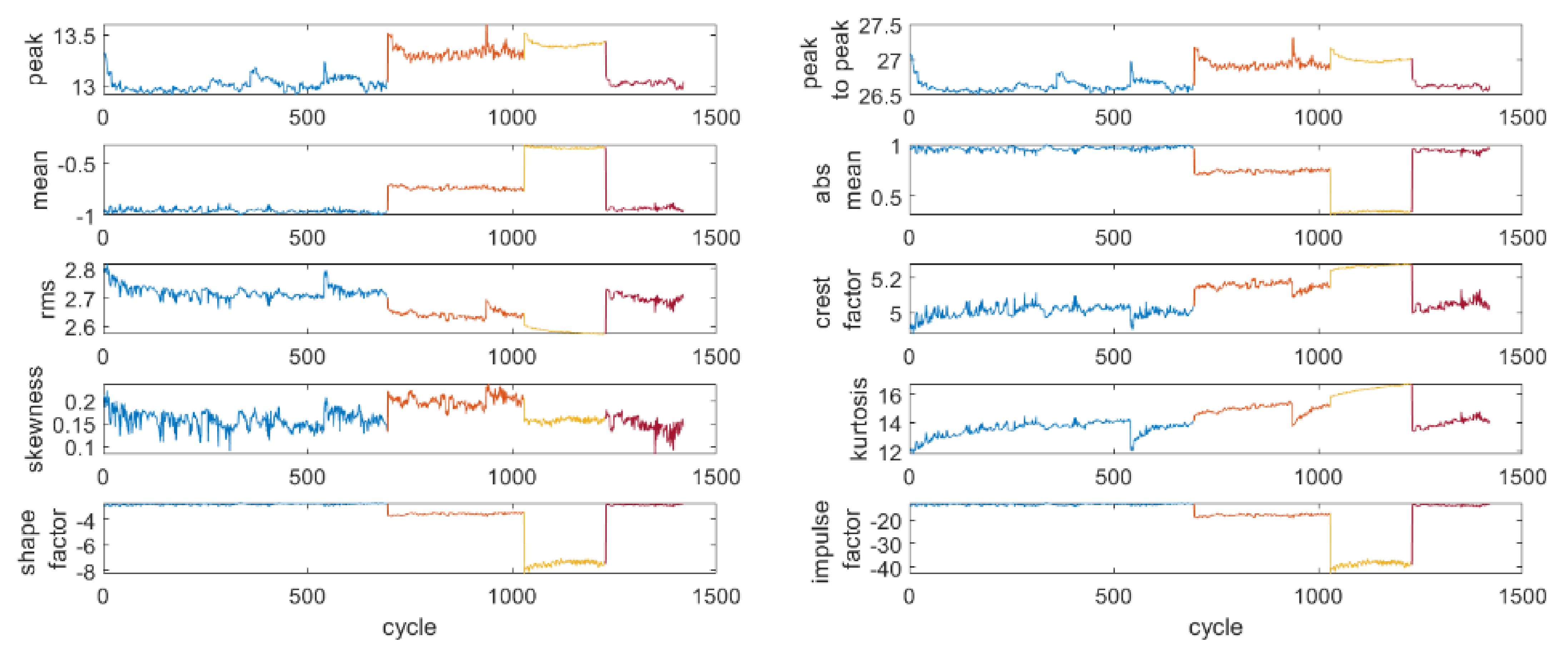
Features are usually extracted in the time, frequency, or time–frequency domain from signal segments of a certain length. In this case, the length is set to 800 ms, equal to the cycle duration. In addition, only time-domain features are extracted, as they require low computational time for calculation and are suitable for streaming applications. In particular, ten typical time-domain features are extracted for each cycle, i.e., peak, peak-to-peak, mean, absolute mean, RMS, crest factor, skewness, kurtosis, shape factor, and impulse factor [38]. The trend of the extracted features in each condition is shown in Figure 5. During the nominal condition, an initial increasing trend can be observed for some features, e.g., kurtosis, which corresponds to the warm-up phase of the machine. Finally, fault 3 is very similar to the nominal condition. Indeed, the signal collected with this sensor is not able to capture the fault information. As the company already provided the susbsyem with another sensor, that collects a signal able to reveal the health condition of the machinery, further investigation using other kinds of features, e.g., extracted in the time–frequency domains, was not performed.

In most ML methods, feature selection before fault diagnosis helps to improve the final classification accuracy [39]. Indeed, feature extraction leads to an increase in the feature vector dimension. However, not all the extract features can affect fault diagnosis. Therefore, the optimal features that have intrinsic information about the faults should be retained [40]. In other words, the information retained in the feature subset must demonstrate sensitivity to variation in events observed by a system [41].

Feature selection aims to reduce the number of variables in a dataset by selecting the more discriminative variables and eliminating the redundant ones [42]. In contrast to dimensionality reduction techniques, feature selection does not apply any transformation to the original feature set. Therefore, feature selection preserves the original physical meaning of each variable. For this reason, it is particularly suitable for fault diagnosis in industrial contexts [43].

Different evaluation measures and search techniques are used to produce a suitable feature subset in feature selection [44]. In this paper, the Pearson correlation analysis and the Recursive Feature Elimination (RFE) have been applied, as they are two widespread approaches used in the context of fault diagnosis. Pearson’s correlation analysis is a filter-based method used for redundancy elimination. It assumes that if two variables have a high linear relationship, they contain redundant information [45]. A fixed threshold usually determines if features are highly correlated or not. The RFE is a supervised feature selection method, which assigns a weight to the features based on a particular classification model and recursively removes the features with the most negligible weight [46].

In the present paper, first, the Pearson correlation is conducted, and a threshold equal to the absolute value of 0.9 is chosen. Then, the correlation matrix is first built using the Pearson correlation coefficient computed among all features and expressed by Equation (1).

$$r_{XY}=\frac{Cov\left(X,Y\right)}{\sqrt{Var\left(X\right)Var\left(Y\right)}}=\frac{{{\displaystyle \sum }}_i(x_i-\overline{x})(y_i-\overline{y}) }{\sqrt{{{\displaystyle \sum }}_j{(x_j-\overline{x})}^2{{\displaystyle \sum }}_k{(y_k-\overline{y})}^2}}$$

(1)

where $X$ and $Y$ are two random variables, $Cov\left(X,Y\right)$ is the covariance of the two variables, $Var\left(X\right)$ and $Var\left(Y\right)$ are the variance of the variable $X$ and $Y$, respectively, $x_i$ and $y_i$ are two observations of $X$ and $Y$, respectively, and $\overline{x}$ and $\overline{y}$ are their mean values. The Pearson correlation coefficient, $r_{XY}$, is always included in the range $\left[-1, 1\right]$, where −1 indicates that the two variables are negatively correlated, 1 indicates that the variables are positively correlated, and 0 that the variables do not correlate. After the correlation matrix construction, an iterative process for feature elimination is conducted. Hence, for each column, and for each row, if $r_{XY}\le -0.9$ or $r_{XY}\ge 0.9$, the column is eliminated.

The Pearson correlation analysis does not consider the effect of each feature on the classification accuracy. For this reason, the RFE, which is a wrapper model, is also applied to evaluate the selected features’ goodness. The model adopted within the RFE is the Decision Tree.

2.1.3. Fault Diagnosis

Three different classification models are trained for the classification of four conditions, i.e., Decision Tree (DT), Support Vector Machine (SVM), and k-Nearest Neighbor (k-NN) [47,48].

A Decision Tree is a classifier expressed as a recursive partition of the instance space. The decision tree consists of a root node that contains all observations. Then, observations are split into nodes according to a specific splitting rule until a defined termination criterion is met. The terminal node is named leaf, in which the observations are assigned to the class representing the most appropriate target value. Alternatively, the leaf may hold a probability vector indicating the probability that the target attribute has a certain value. The probability is estimated as the class frequency among training instances that belong to the leaf for each leaf. One of the parameters affecting the complexity of the tree is its depth, which is usually considered in the hyper-parameters optimization process to find the best trade-off between prediction accuracy on the training set and the generalization error.

The Support Vector Machine (SVM) is, in its initial version, a two-class linear classifier, in which the learning process consists of designing a hyperplane that maximizes the margin given by the distance between the hyperplane and its closest observations, i.e., the support vectors, in the features’ space while maintaining the correct class division. When the dataset is not linearly separable, the system can incorrectly classify some observations and pay the price, called penalty error (C), in the objective function. In addition, non-linearly separable original space might be transformed into a linearly separable space through the use of a kernel. Different kernel functions are used in SVMs, such as linear, polynomial, and Gaussian Radial Basis Function (RBF). The selection of the appropriate kernel function is crucial, as the kernel defines the feature space in which the training set observations will be classified. For this reason, the kernel and the penalty error are the primary hyperparameters to optimize.

k-Nearest Neighbor algorithm is an instance-based learning algorithm in which new observations are classified by comparing them with the most similar in the training set. The assumption is that input data of the same class should be closer in the features space. Therefore, for a new input data, the algorithm computes the distance between the data itself and all the observations of the training set: the new observation will be assigned to the class of its k nearest neighbors. Alternatively, the method can make discrete predictions by reporting the relative frequency of the classes in the neighborhood of the prediction point. The number of neighbors, k, is a critical issue as it highly affects classification accuracy. Large values of k reduce the effect of outliers but reduce the boundaries evidence between two classes; on the other hand, small values of k increase the probability of overfitting the data. Hence, the optimal value k needs to be determined.

For the training of each model, the k cross-validation with k = 10 is used to prevent overfitting, while the Grid Search (GS) [49,50] is used for hyperparameters optimization.

Table 2. Hyperparameter range values.

Model	Hyperparameter	Range
Decision Tree	Maximum depth	{1 – 15, 20}
Support Vector Machine	C Kernel	{1, 5, 50, 100, 500, 1000} {linear, rbf, polynomial}
k-NN	K	{1 – 15, 20}

shows the set of hyperparameters used for each model and the values range. In particular, the polynomial kernel function considered in the SVM is a third-degree function, and the $\gamma$ value used in the Radial Basis Function (RBF) kernel function is equal to $\gamma =\frac{1}{2{\sigma }^2}=\frac{1}{\left(n_{features}\ast {{\displaystyle \sum }}_j{(x_j-\overline{x})}^2\right)}=$, where ${\sigma }^2$ is the sigma square value, $n_{features}$ is the number of features, and ${{\displaystyle \sum }}_j{(x_j-\overline{x})}^2$ is the variance of input variable $X$.

In order to evaluate the performance of each classifier, several parameters can be defined. Here, precision and recall are considered. Precision measures how many samples classified in the positive class are positive, and it is computed through Equation (2). Finally, the Recall, also named Sensitivity or Probability of Detection, measures how well the classifier recognizes the positive samples, and is defined in Equation (3).

$$Precision=\frac{TP}{FP+TP}$$

(2)

$$Recall=\frac{TP}{FN+TP}$$

(3)

where:

• $TP$ (True Positive) is the number of observations correctly classified as positive;
• $FP$ (False Positive) is the number of negative observations classified as positive;
• $FN$ (False Negative) is the number of positive observations classified as negative.

2.1.4. Anomaly Detection

Three different anomaly detection algorithms are trained to determine the most suitable model for detecting anomalous behaviors. Hence, models are only trained on the nominal class, and then they are tested and evaluated using two different metrics.

First, a variant of the traditional k-means clustering method is applied. K-means is a distance-based algorithm that requires only the number of clusters, $\mathrm{k}$, to be set a priori. For novelty detection, k-means is trained only on a small subset of the available nominal dataset ($\mathrm{k}=1)$. In this application, the training set size is set equal to 100 cycles. Then, to make it suitable for streaming applications, a sliding window method is used. Hence, for each new data sample, the previous $x$ data samples and the current sample are input to the algorithm. The sliding window method ensures a faster application, as it is able to keep only the last $x$ values in memory, instead of the whole dataset. In this application, a sliding window including ten points is considered. In addition, the algorithm makes the inference only on one point at iteration as the $x$ values have all been already assigned, except the last one, that is, the current one. Finally, as the classic k-means is expensive for large datasets, the mini-batch k-means (MBKm) proposed in [51] is used for streaming novelty detection.

The second trained model is the One-Class Support Vector Machine (OCSVM). Unlike traditional SVM, the training phase of the OCSVM consists of finding the boundary, i.e., the margin, that accommodates most of the training points. Test data samples are then considered outliers if they fall beyond the identified boundary [52]. Even in this case, to make the algorithm work in streaming, a sliding window is considered during model application.

Finally, the last trained model for anomaly detection is an ensemble of autoencoders. Among classification-based models, Deep Learning, and in particular autoencoders, showed better performance than conventional methods in various real-world applications [53]. The autoencoder is a neural network composed of two parts. The encoder part transforms the large-dimensional input data into a small set of features, while the decoder part reconstructs the data from the extracted features, generating a reconstruction error. In this application, the ensemble of autoencoders, named kitNET [54], is used. In this architecture, a feature mapper level maps the input features into $\mathrm{k}$ sub-instances, one for each autoencoder in the next level. The ensemble of autoencoders constitutes the anomaly detector, which aims to detect the anomalies based on a threshold on the reconstruction error, which is expressed in terms of Root Mean Square Error (RMSE). The training phase takes place in the ensemble layer, in which the autoencoders learn the nominal behavior of the input sub-instances and reconstruct the input minimizing RMSE. Then, the minimum RMSEs are sent to the output layer, which is responsible for the anomaly score assignment during the execution phase. The higher the error, the higher the anomaly score of the test samples. In this application, the threshold on the reconstruction error is set equal to 0.5, while the number of autoencoders is set to 10. For the training phase, 500 nominal observations are used.

In order to evaluate how well the trained models recognize anomalies, two metrics have been used, i.e., the probability of detection, or recall, and the false positive rate ($FPR$) The first metric is computed through Equation (3).

The second metric evaluates how well the model recognizes the nominal observations and is defined by Equation (4). In other words, a high value of this metric implies a high number of false alarms, i.e., points belonging to the nominal class, recognized as anomalies by the model [55].

$$FPR=\frac{FP}{FP+TN}$$

(4)

where $TN$ (True Negative) is the number of observations correctly classified as negative.

2.1.5. Online Condition Monitoring

The output of the offline training consists of (1) the best feature subset, which contains the minimum information for class separation; (2) the best classification model, which can accurately classify the known conditions in a short time; and (3) the best anomaly detection model, which can distinguish the nominal condition from all other conditions. These outputs will be used in the online phase to assess the current condition of the monitored machinery and establish if a novel behavior occurred.

In the online phase, data are collected continuously in streaming, while the online inference is made by the fault detection and diagnosis models at each cycle. Hence, the selected feature subset is extracted every 800 ms, and the so-obtained feature vector is input to the anomaly detection model, which determines if it belongs to the nominal class or not. In the first case, the algorithm ends and goes to the next cycle. Otherwise, a counter is incremented by one, and the algorithm goes to the next cycle. When the value of the anomaly counter is equal to 2, the trained classification model is applied to determine the belonging class of the past two points. Then, if the maximum Class Probability Estimation (CPE) is higher than a certain threshold, the fault has been diagnosed, and the machine can be stopped. Otherwise, the detected anomaly does not correspond to any of the known conditions. In this case, an alarm is triggered, and a check by the machine user may be required to determine whether the novel behavior is a fault condition or not.

3. Results

In this section, the main results of the present study are provided. First, datasets corresponding to all available machinery conditions are considered in the training phase in order to select the best feature subset, the best classification model, and the best anomaly detection model in the hypothesis to know all the machinery behaviors. In this scenario, the online monitoring phase has the only objective of identifying points corresponding to a condition change as anomalies and classifying them in the correct fault class. Note that one dataset for each condition (e.g., dataset D1 for the nominal condition) is considered for the training, except for fault 2, for which the only available dataset is used for both training and online testing. In a second scenario, fault 2 has been removed from the training dataset to evaluate the novelty detection ability of the methodology. The datasets used in both scenarios for the training and the online testing are summarized in

Table 3. Testing Scenarios.

Scenario	Training Datasets	Online Testing Datasets
1	D1 + D2 + D3 + D5	D1 + D7 + D8 + D2 + D9 + D4 + D6 + D3 + D5 + D10
2	D1 + D2	D1 + D7 + D8 + D2 + D9 + D4 + D6 + D3

.

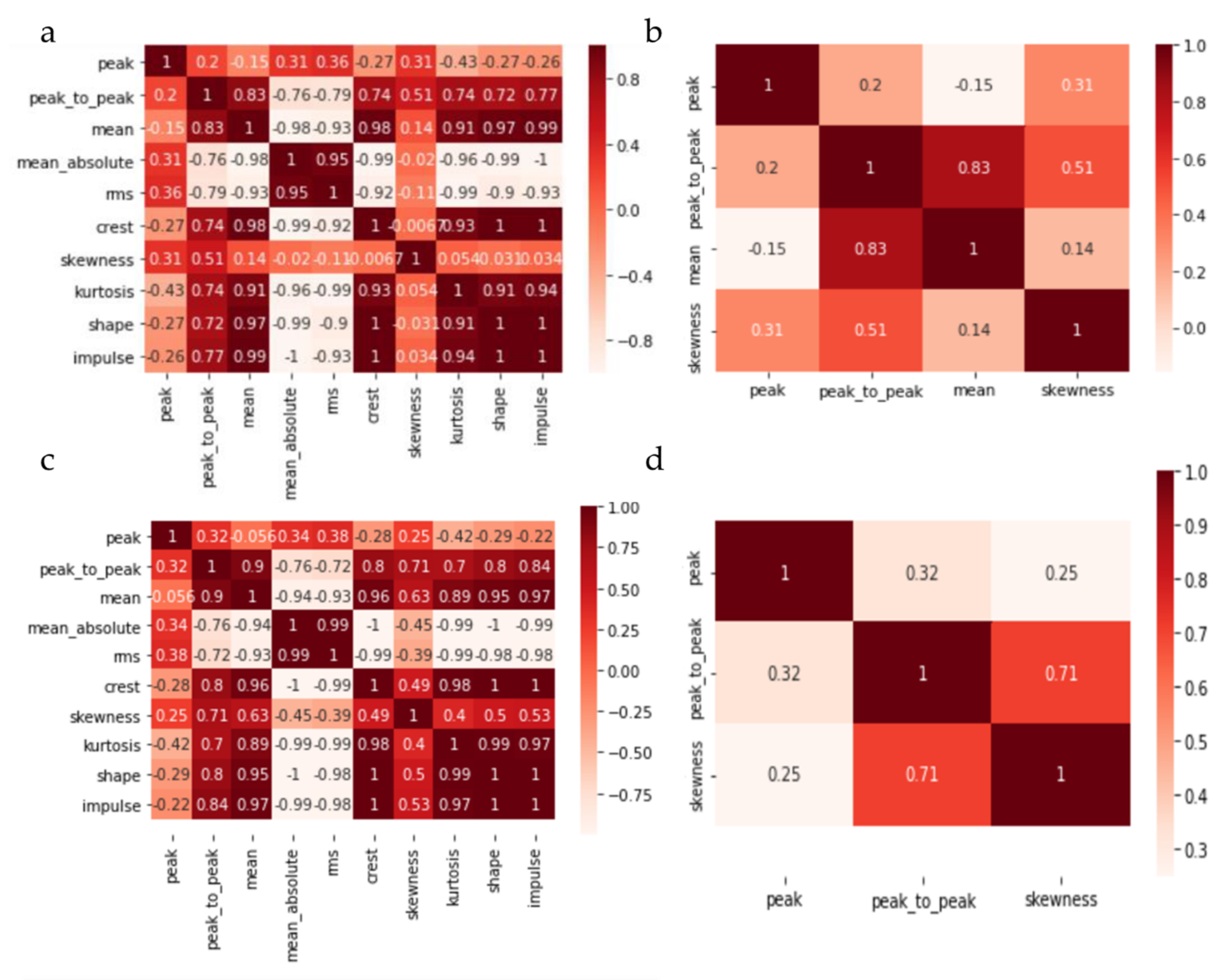
The feature subset represents the first output of the methodology described in previous sections. The ten statistical features extracted in the time domain (see Section 2.1.2) are used to build the Pearson correlation matrices of both scenarios, shown in Figure 6a,c, respectively. It can be seen that, in both cases, some of the extracted features have a high correlation, such as the mean and the mean of the absolute values, which have a correlation coefficient equal to −0.98 (Figure 6a). In this case, the mean absolute on the column is eliminated, while the mean on the raw is kept. This process is repeated until the whole matrix is analyzed. In the end, for scenario 1, only four features, i.e., peak, peak to peak, the mean, and the skewness, are selected, whose correlation coefficients are shown in Figure 6b. For scenario 2, the peak, peak to peak, and the skewness are selected (Figure 6d). As the described method is affected by the features’ order in the correlation matrix, the Pearson correlation analysis is repeated after randomly changing the features’ order. In this case, instead of the mean value, the shape factor has been selected. However, the mean correlation index, computed as the arithmetic mean of the absolute values of the Pearson coefficients in the correlation matrix, is similar in both matrix configurations. To further evaluate the goodness of the selected features, the RFE algorithm is applied, which assigns a score equal to 1 to both feature subsets selected through the Pearson correlation analysis. This score confirms that the selected features have a low correlation and positively contribute to the classification accuracy.

The fault classification model represents the second output of the methodology. Several considerations lead to choosing a model rather than another. First, the best model should have the highest precision and recall. In addition, as the selected model will be applied to streaming data and provide real-time results, the execution time, i.e., testing time, is also critical. Finally, the model should potentially deal with an infinite amount of data. Hence, it has to be scalable and trained on a large data set quickly.

Table 4. Fault diagnosis performance of scenario 1 (S1) and scenario 2 (S2).

		Scenario 1			Scenario 2
Model	Hyperparameters (Hyp.)	Optimal Hyp.	Precision	Recall	Optimal Hyp.	Precision	Recall	Velocity and Scalability
DT	Maximum depth	9	92.3%	92.5%	5	100%	100%	High
SVM	C Kernel	1000 RBF	95.0%	93.6%	1 Linear	100%	100%	High
k-NN	K	3	95.1%	93.7%	1	100%	100%	Low

summarizes the results in terms of precision, recall, and velocity and scalability, obtained from the application of the grid search algorithm. In addition, the selected hyperparameters for each model are also present in the table. In scenario 1, the model with the best precision and recall is the k-NN that, with $\mathrm{k}=3$, achieves the 95.1% of precision and the 93.7% of recall. However, k-NN has low scalability, as it computes the distance between a point and all other points at each iteration, making the process time-consuming for large datasets. Similar performances are also provided by the SVM, which has high scalability. In addition, its execution time is equal to 0.02 s. However, the basic SVM does not provide the class estimation probability. As one of the main goals of the present study is to provide an industrial solution that is easy to implement, and as both precision and recall of DT are slightly worse than those of the SVM, the DT has been chosen for the online fault diagnosis. In scenario 2, all models have the 100% of precision and recall.

The last output of the training phase is the model selection for real-time anomaly detection. The three models introduced in Section 2.1.4 are evaluated in terms of the metrics defined by Equations (3) and (4). In addition, they are also compared in terms of execution time as they have to process streaming data and provide real-time feedback. The application of mini-batch k-means, one-class SVM, and kitNET led to the results summarized in

Table 5. Parameters and results of the mini batch k-means of scenario 1 (S1) and scenario 2 (S2).

		Scenario 1			Scenario 2
Parameter	Value	Execution Time (sec)	$\mathrm{Recall}$	$\mathrm{FPR}$	Execution Time (sec)	$\mathrm{Recall}$	$\mathrm{FPR}$
K	2	6.7	0.3%	37.21%	1.98	0.41%	10.38%
Initialization time	100 cycles
Amplitude of the sliding window	10

,

Table 6. Parameters and results of OC-SVM of scenario 1 (S1) and scenario 2 (S2).

9		Scenario 1			Scenario 2
Parameter	Value	Execution Time (sec)	$\mathbf{Recall}$	$\mathbf{FPR}$	Execution Time (sec)	$\mathbf{Recall}$	$\mathbf{FPR}$
Initialization time	100 cycles	1.2	100%	61.42%	0.13	97.2%	-%
Amplitude of the sliding window	10

and

Table 7. Parameters and results of kitNET of scenario 1 (S1) and scenario 2 (S2).

9	Scenario 1				Scenario 2
Parameter	Value	Execution Time (sec)	$\mathbf{Recall}$	$\mathbf{FPR}$	Value	Execution Time (sec)	$\mathbf{Recall}$	$\mathbf{FPR}$
Initialization time (feature mapping)	100 cycles	0.13	100%	6.54%	100 cycles	0.04	100%	0%
Initialization time (anomaly detection)	400 cycles				400 cycles
Number of autoencoders	10				10
Threshold	0.5				0.5

, respectively. In addition, the parameters set by the user for each model are also present.

In both scenarios, kitNET is the best model from all perspectives. It is fast, has the highest recall and the lowest false positive rate. On the contrary, the mini batch k-means has low values of recall, and the value of the false positive rate is lower than the FPR of the OCSVM in the first scenario. In the second scenario, the FPR of OCSVM cannot be computed, as both false positives and true negatives are equal to zero. As a result, the kitNET has been chosen for the online monitoring.

After the training phase, the online condition monitoring has been tested. The pseudo-code of that phase is shown in

Table 8. Pseudo-code of the online condition monitoring.

Initialize:

Input: Optimal feature subset, cycle duration ($d$), trained DT, trained kitNET, Anomaly threshold $(T{h}_a)$ classification threshold $\left(T{h}_c\right)$

While $i<d$

Do nothing

$k=1$

Compute optimal features

Apply kitNET and assign the anomaly score

If anomaly score $<(T{h}_a)$

Increment $k$ by 1

End

Else

Increment $a$ by 1

End

If $a\ge 2$

Apply DT and compute the CPE for each known class $c$

If $\underset{c}{\max }CPE>\left(T{h}_c\right)$

If $\underset{c}{\max }CPE$ for $c$ = nominal

Increment $k$ by 1

End

Else

Fault corresponding to class $c$ occurred

Stop the machinery

Break

Else

A possible novel behavior has been detected

Generate an alarm

Break

End

End

. For the scenario 1, the data flow has been generated by sequence the observations corresponding to the nominal condition (D1 + D7 + D8), fault 1 (D2 + D9), restored condition (D4 + D6), fault 2 (D3), and fault 3 (D5 + D10). In scenario 2, the online testing has been carried out on datasets D1, D7, D8, D2, D9, D4, D6, and D3. The first 300 cycles are used for the initialization. Hence, the anomaly detector is only activated after 300 cycles. Then, at each iteration $\mathrm{k}$, i.e., every 800 ms, the following steps are carried out.

First, the selected features are extracted. Then, the feature vector is input to kitNET, which computes the anomaly score. If the reconstruction error is lower than the fixed anomaly threshold $(T{h}_a)$, the feature vector is considered nominal, and the algorithm goes to the next iteration. If the reconstruction error is greater than or equal to $T{h}_a$ for two consecutive feature vectors (stored in the counter $a$), the feature vectors are input to the Decision Tree, which assigns the class probability membership to the labeled observations. If the maximum probability is greater than the fixed classification threshold $\left(T{h}_c\right)$, the predicted class is considered accurate. Hence, if the predicted class is nominal, the algorithm goes to the next iteration. Otherwise, a warning message indicating the occurred fault is generated, and the machinery is stopped. If the maximum probability is lower than $T{h}_c$, a possible novel behavior occurred, and a human check may be required to establish the anomaly’s cause. Note that the choice of the minimum number of detected anomalies that have to occur before the classifier activation is made with the goal of finding a good trade-off between the false alarm rate and the latency of the classifier. A single anomaly would generate a greater probability of error. On the other hand, if the classifier is activated after more than two anomalies, the fault or the novel behavior would be recognized after three cycles. In this case, it would mean that at least 12.8 products would be discarded for quality issues.

Note that the algorithm was not stopped in the online condition monitoring if a known fault was recognized in order to test the methodology. However, in real applications, if a fault is detected, the machinery should be stopped as soon as possible.

In the first scenario, the algorithm correctly classified observations belonging to the nominal class, fault 1, and fault 2. On the contrary, the change from the restored condition and fault 3 was not detected. Hence, observations belonging to fault 3 were wrongly considered nominal. Moreover, in eighteen cases, the kitNET detected two anomalies in a row. However, the DT classified them as nominal with a class probability membership value equal to 1. Therefore, no alarm was generated. Note that, as models were trained with four classes in this scenario, the classification threshold was set equal to 0.5.

In the second scenario, observations belonging to the nominal condition and fault 1 were correctly classified. When fault 2 occurred, the kitNET detected two anomalies in a row. Hence, the DT was applied, which assigned a class probability value of 0.87 and 0.13 for the fault 1 and nominal class, respectively. As models were trained with only two classes in this scenario, the classification threshold was set equal to 0.9. Hence, when fault 2 occurred, an alarm indicating that a possible novel behavior occurred was generated.

4. Discussion and Conclusions

The results presented in the previous section led us to draw several considerations.

First, the computational time for both training and online condition monitoring is low. In particular, in the online monitoring, the inference by the classification models is only made when anomalies are detected. Indeed, a streaming labelling of nominal data might not be necessary as, in many industrial situations, nominal data are much easier to collect. Therefore, the lack of nominal data labelling allows reducing the computational time of online monitoring, which is less than 7 s in the first scenario and less than 3 s in the second scenario. In addition, when a novel behavior is detected, the classification model can be re-trained only adding the samples corresponding to the fault conditions to the already available dataset. In this way, it is not necessary to keep in memory all nominal samples, which represents an advantage for edge applications, in which the storage memory is limited.

Second, the high values of precision and recall obtained on the test set demonstrate the high generalization ability of the selected model for fault diagnosis. Indeed, the datasets used for the training and the online monitoring were different in most cases. For each condition, except for fault 2, datasets were collected on different days. For instance, D1 and D7 were both collected in the nominal condition. However, only D1 was used in the training phase.

Third, results demonstrate that the classification accuracy is not affected by transients. Indeed, most datasets contain the warm-up phase of the machinery. However, thanks to the feature selection steps and, in particular, to the RFE technique that uses a classification model to identify the best feature subset, the increasing trend of some extracted features that can be seen at the beginning of each dataset (see Figure 5) does not influence the classification accuracy. Avoiding the pre-processing step on the available datasets is an essential aspect in real applications, where many transients could be present.

Finally, an evident positive aspect is the minimization of false alarms. First, using kitNET for anomaly detection, the false positive rate is equal to 0%. Second, the use of a classifier after the anomaly detection has a double function. On the one hand, it allows classifying the observations in one of the known fault classes. Hence, it makes possible the diagnosis of the detected anomaly. On the other hand, it allows classifying the detected anomalies in the nominal class if the anomaly detector made an error.

Another important consideration is related to the feature selection phase. In particular, two different feature subsets are selected in the two scenarios, i.e., peak, peak-to-peak, mean, and skewness in the first scenario, and peak, peak-to-peak, and skewness in the second scenario. Hence, in the hypothesis that fault 2 is unknown, i.e., the training is based only on datasets corresponding to the nominal condition, and fault 1, only three features would be selected. Nevertheless, the anomaly corresponding to the occurrence of fault 2 is detected. On the contrary, the extracted features are not able to recognize fault 3. However, as suggested by the company’s technical office, fault 3 can only be seen by monitoring another kind of parameter with another type of sensor.

The last consideration is related to the anomaly threshold $T{h}_a$ and the classification threshold $T{h}_c$, which the user in the present paper manually sets. The anomaly threshold can be considered an inherent parameter of kitNET and, as such, could be tuned through several optimization techniques. A more critical parameter is the classification threshold, as it affects the ability to detect novelties. In general, it should be higher when models are trained with few classes. However, a limitation of the proposed methodology lies in the absence of a generalizable way to set this parameter.

We can conclude that the methodology is easy, fast, and accurate. It can detect anomalies corresponding to known faults and to novel behavior during the online monitoring of the sealing sub-system of a packaging machine. Few training data guarantee a high accuracy and a high generalization ability of the classification models. The integration of a classifier and an anomaly detector effectively reduces the false alarms and the computational time. Future developments of the current research will be dedicated to application of DL for anomaly detection to raw signals in order to eliminate its dependency on extracted features and increase the classification accuracy [56].