Comparison of Twelve Machine Learning Regression Methods for Spatial Decomposition of Demographic Data Using Multisource Geospatial Data: An Experiment in Guangzhou City, China

Abstract

The spatial decomposition of demographic data at a fine resolution is a classic and crucial problem in the field of geographical information science. The main objective of this study was to compare twelve well-known machine learning regression algorithms for the spatial decomposition of demographic data with multisource geospatial data. Grid search and cross-validation methods were used to ensure that the optimal model parameters were obtained. The results showed that all the global regression algorithms used in the study exhibited acceptable results, besides the ordinary least squares (OLS) algorithm. In addition, the regularization method and the subsetting method were both useful for alleviating overfitting in the OLS model, and the former was better than the latter. The more competitive performance of the nonlinear regression algorithms than the linear regression algorithms implies that the relationship between population density and influence factors is likely to be non-linear. Among the global regression algorithms used in the study, the best results were achieved by the k-nearest neighbors (KNN) regression algorithm. In addition, it was found that multi-sources geospatial data can improve the accuracy of spatial decomposition results significantly, and thus the proposed method in our study can be applied to the study of spatial decomposition in other areas.

1. Introduction

Information about fine-scale population distribution is essential in many areas, including urban planning and management [1], natural disaster response [2], infectious disease prevention and control [3], resource allocation, and environment protection [4]. Accurate population distribution data are fundamental for the achievement of urban sustainable development goals (SDGs) [5,6]. The census method is the main way to collect population data in varying countries. However, the spatial resolution and update frequency of census data are too low to meet the requirements of modern urban governance. Due to the fact that demographic data is usually collected in subdistrict units, the spatial decomposition of demographic data into gridded population data can show population distribution patterns more accurately [7,8,9,10,11]. Therefore, fine-scale and accurate population information is essential for exploring the relationship between urban residents and the built environment [1]. Guangzhou, the capital city of Guangdong Province, is facing several challenges, such as a large population and huge pressure on its resources and environment. Therefore, fine-scale gridded population distribution information is particularly critical for improving the quality of urban governance.

There have been many achievements in the field of spatial decomposition of demographic data. The spatial decomposition methods of demographic data are mainly divided into spatial interpolation [12,13,14,15] and dasymetric mapping [14,16,17]. The gridded population data is usually produced by integrating several auxiliary data and using several interpolation methods, such as inverse distance weighted (IDW), kriging, et. al. Dasymetric mapping is a geographic information technique for disaggregating demographic data into more homogenous units by incorporating additional data [18]. The typical global gridded population datasets mainly include the Gridded Population of the World (GPW) [19], the Global Rural-Urban Mapping Project (GRUMP) [2], LandScan Global [20], Global Human Settlement Population Grid datasets (GHS-POP) [21], and Worldpop [22]. However, most of these datasets are designed for extensive coverage and free accessibility for the undeveloped regions in the world; their accuracy on a local scale, such as that of a city or subdistrict, still need to be analyzed [23,24].

In fact, the spatial decomposition of demographic data from coarser units into finer unit is a regression process according to the weight layer. Several regression models have been proposed to produce decomposition results, such as ordinary least squares (OLS) regression, random forest (RF) regression [25,26], and so on. In general, regression models are usually divided into linear and nonlinear models. The OLS model is a classic linear regression algorithm, but it easily causes overfitting problems. Subsetting and regularization are common methods used to correct this. The best subset regression (BSR) is a widely used method for the selection and estimation of the parameters in a linear model, dating back at least as far as Beale, Hocking and Leslie [27,28,29], that tries all possible combinations of variables and chooses one that minimizes certain criteria. Least angle regression (LARS) is a method of variable selection proposed by Bradley Efron et al., in 2004, which is similar to the form of forward stepwise regression [30]. The commonly used regularization functions include L1 and L2 regularization. The regression methods that use L1 regularization and L2 regularization are called Lasso Regression [31,32] and Ridge Regression [33,34], respectively. Elastic Net is a linear regression model that uses both the L1 norm and the L2 norm of the coefficient vector [35,36,37]. It is especially suitable for occasions when multiple features are related to each other. As we know, the collinearity of the independent variables is also the main reason for the over-fitting problem of linear regression. Principal component regression (PCR), derived from the principal component, is a useful method for dealing with collinearity [38,39]. However, the regression model obtained with principal components is not as easy to explain as the regression model established with the original independent variables. Partial least squares (PLS) regression [40] is a variant of PCR regression in which the projection is applied to both the independent variable and the dependent variables. Therefore, the PLS method is also considered as a bilinear factor model. Random sample consensus (RANSAC) [41,42] is a method that can estimate the parameters of the mathematical model in an iterative way from a set of observation data sets containing “outliers”.

Beside linear regression algorithms, non-linear regression algorithms have received increasing attention in the spatial decomposition of demographic data, especially the random forest model. Yao et al. [10] downscaled demographic data into a building-scale gridded population map based on the random forest algorithm by using various geospatial data sets, such as POI data, Tencent online user densities data, and so on. Yao’s study achieved the best accuracy at the community scale through comparison with six other decomposition methods, including areal weighting, binary dasymetric mapping, interpolation with cokriging, and so on. Wang et al. [43] integrated Luojia 1-01 night light remote sensing images, POI data, and Sina Weibo check-in data, and converted the Zhejiang province’s demographic data into a fine grid scale by using the random forest model. The effectiveness and superiority of the random forest model was proven again by Wang’s research, which found that its accuracy was higher than that of the WorldPop dataset and previous density-based studies. Zhou et al. decomposed Chongqing’s demographic data into gridded population data by using the random forest regression model and multi-source geospatial data. The model evaluation results of Zhou’s study once again confirmed the superiority of the random forest model over other regression models. However, the application of non-linear regression models other than random forest in the spatial decomposition of demographic data still needs to be strengthened.

In addition, most existing studies only use one or two regression algorithms, and comparative studies of different regression algorithms in the spatial decomposition of demographic data are still relatively rare. To solve the problem, we applied twelve commonly used regression algorithms to generate the gridded population data of Guangzhou city, China, with a resolution of 150 m, and compared their performance using several evaluation metrics. The findings of our study can be used for fine-scale population mapping in Guangzhou or another city.

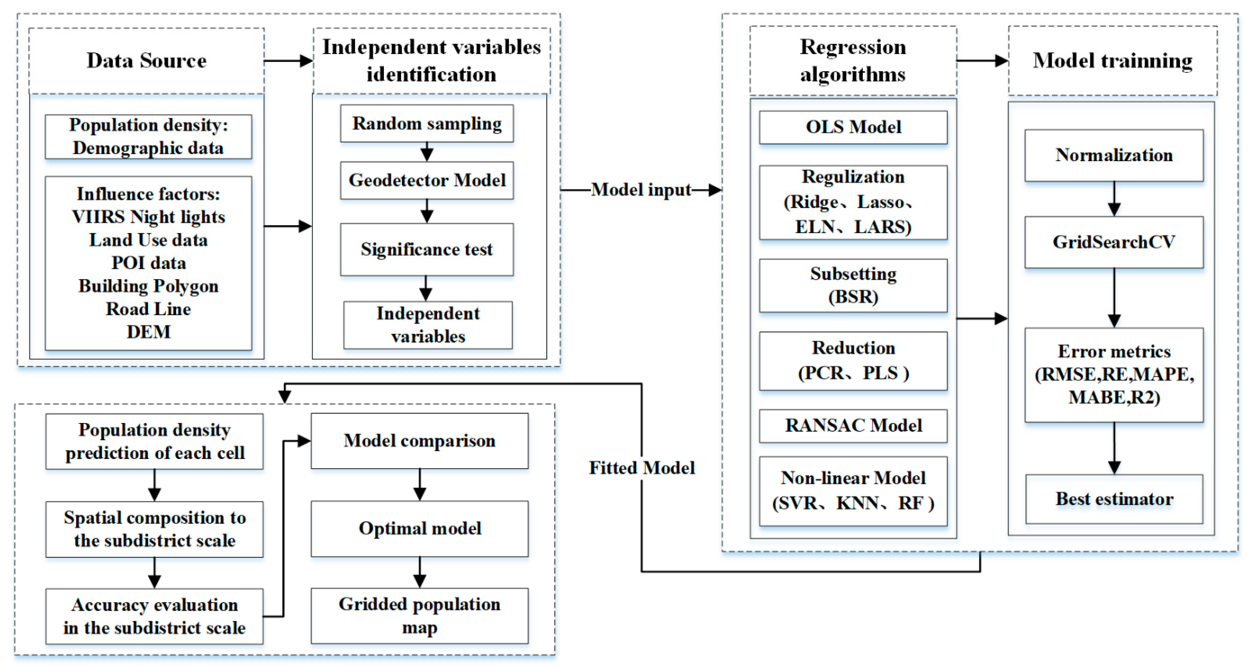
2. Materials and Methods

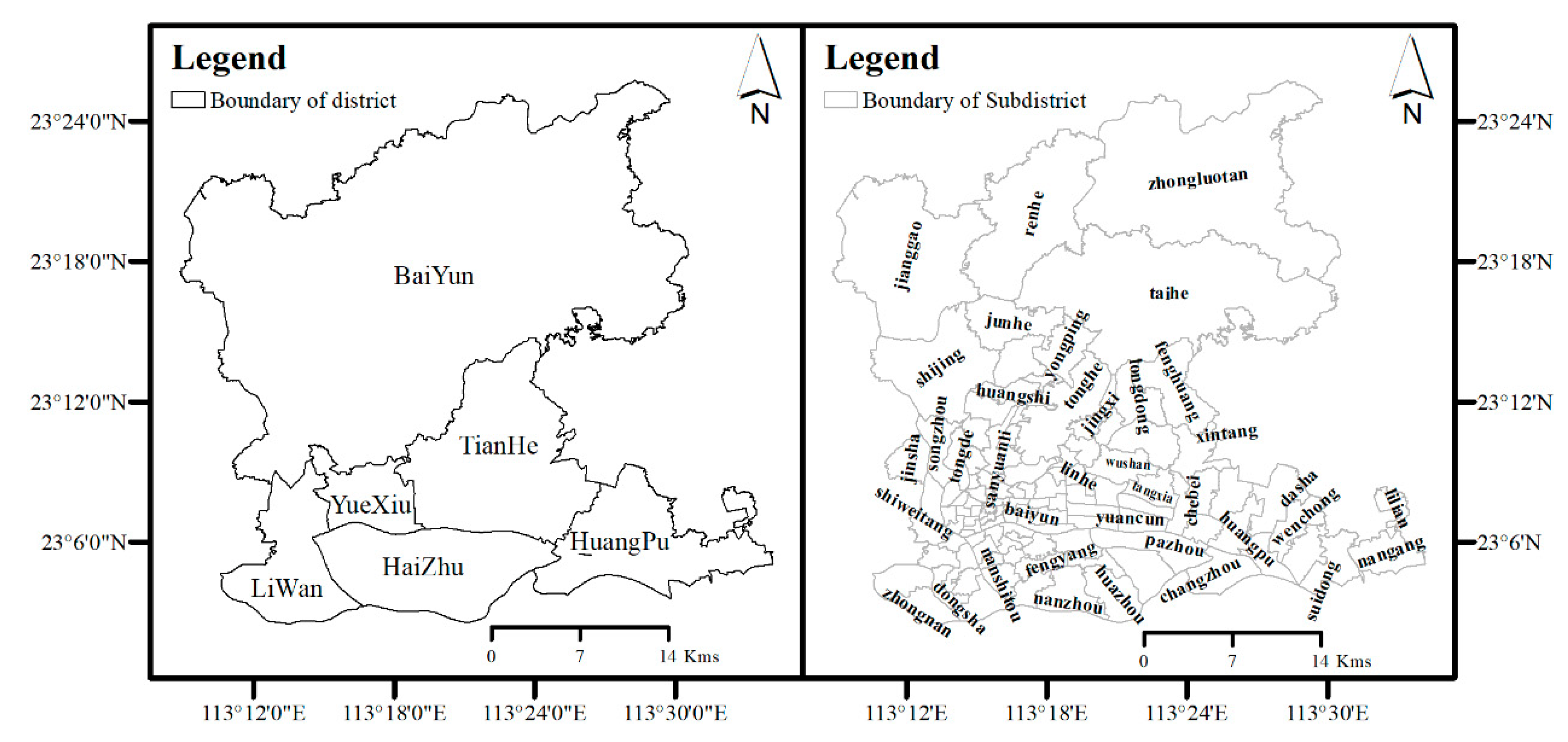
2.1. Study Area and Data Sources

Guangzhou city is located in the middle of Guangdong Province, China, with an east longitude of 112°57′–114°3′, and a north latitude of 22°26′–23°56′. The study area is composed of six districts in Guangzhou city (including YueXiu district, LiWan district, TianHe district, HaiZhu district, HuangPu district, and BaiYun district), encompassing the city’s main urban area. The population density of the study area is highest in Guangzhou city. According to demographic data from 2013, the study area contains a population of about 4.77 million, in an area of more than 1057 km². A subdistrict is a basic administrative division of Chinese cities that is generally smaller than a district. According to statistics on the population density of subdistricts, more than 60% of the subdistricts in the study area feature a population density of less than 17,000 people per square kilometer. The subdistricts with a population density between 17,000 and 60,000 people per square kilometer occupy nearly 28.2%. Less than 9% of the subdistricts feature a population density of more than 60,000 people per square kilometer. In general, the study area is dominated by subdistricts with a medium population concentration. The study area map is shown in Figure 1.

The demographic data of each subdistrict in 2013 were collected from Guangzhou municipal public security bureau. The administrative boundary data and road line data were digitized in 2014 from Amap, one of China’s popular web mapping services, which is also known as Gaode in Chinese. The website of Amap is https://ditu.amap.com/ (accessed on 9 September 2014). The digital elevation model (DEM) data from 2014 were provided by the Chinese geospatial data cloud, which is a popular geospatial data portal in China (http://www.gscloud.cn/search (accessed on 13 January 2019)), with a spatial resolution of 30 m. The 30 m land use dataset from 2015 was collected from the resource and environment science and data center of China (http://www.resdc.cn/ (accessed on 20 November 2018)). There are six major types of land use: cultivated land, forest land, grassland, water area, urban and rural, industrial and mining, residential land, and unused land. Fourteen types of point of interest (POI) data were collected from Amap in 2015, including catering facilities, public service facilities, companies, shopping facilities, transportation facilities, finance facilities, educational, scientific and cultural facilities, commercial residential facilities, living service facilities, sports and leisure facilities, medical service facilities, government agencies, and accommodation service facilities. The building polygon data were produced according to the national geographic survey data of China. The NPP/VIRRS night light data from 2016 were provided by the national oceanic and atmospheric administration of America (https://ngdc.noaa.gov/eog/viirs/download_dnb_composites.html (accessed on 6 December 2018)), with a spatial resolution of 500 m.

2.2. Methods

The diagram of the technology roadmap for the gridded population mapping is shown in Figure 2. The research process is explained in detail below.

2.2.1. Calculation of Initial Influence Factors in the Grid Scale

As we know, the accuracy of the spatial decomposition results of the demographic data is not only related to the decomposition model, the resolution, and the quality of the data source, but also to the cell size. Therefore, determining the appropriate cell size is the first step in the spatial decomposition of demographic data. According to a previous study [23], the cell’s area should be close to 10% of the smallest subdistrict are in the overall study area. Hence, the cell size of 150 m was chosen for our study. Based on previous research experience, 24 initial influence factors were selected from two groups: natural factors and socio-economic factors. The 24 initial influence factors are shown in

Table 1. Initial influence factors.

Type	Factors
Natural factors	(1) POI density: X1 (Government agencies), X2 (Public service facilities), X3 (Commercial residential facilities), X4 (Medical service facilities), X5 (Financial facilities), X6 (Transportation facilities), X7 (Educational, scientific, and cultural facilities), X8 (Sports and leisure facilities), X9 (Living service facilities), X10 (Catering facilities), X11 (Companies), X12 (Accommodation service facilities), X13 (Shopping facilities) (2) Night light intensity: X14 (Night light intensity index) (3) Building area: X17 (Building area index) (4) Road intensity: X20 (Road density index)
Socio-economic factors	(5) Land use: X15 (Index of urban land use), X18 (Index of arable land), X19 (Index of wood land), X21 (Index of rural land), X22 (Index of other construction land), X23 (Index of waters), X24 (Index of grass land) (6) Altitude: X16 (Elevation index)

. The calculation methods for the factors in the unit of each cell were as follows. Road index is equal to the quotient of road length and cell’s area. Land use index is equal to the ratio of each type of land use to total area of land use polygon. Night light intensity index is calculated as the average night light intensity in the cell. Elevation index is calculated as the average elevation of cell. Building area index denotes the ratio of the building area and cell’s area. Fourteen types of POI index were calculated as the average density of each type of POI in the unit of each cell.

2.2.2. Selection of Independent Variables Based on Geographical Detector Model

The geographical detector model proposed by Wang Jinfeng et al. [44] is a widely used geospatial model for spatial stratified heterogeneity analysis, since this method with no linear hypothesis has an elegant form and a definite physical meaning [45]. A factor detector, one of the sub-detectors in used in geographical detector models, was used in our study. First, 3000 sample points were randomly selected in the study area. Second, the population density of sample points was chosen as the dependent variable of the factor detector, while the 24 influence factors’ values of sample points were chosen as independent variables. Next, the q-statistic values of the 24 influence factors, which denoted the power of determinant, were calculated using the factor detector tool in GeoDetector. Finally, all the influencing factors with q-statistical values greater than 0.1 and p values significant at the level of 0.05 were selected as independent variables for the subsequent regression analysis.

2.2.3. Spatial Decomposition of Demographic Data Using Different Regression Algorithms

Machine Learning Training Method

The values of nineteen independent variables for each subdistrict were obtained by using the zonal statistics function of ArcGIS 10.8 software. The independent variables values were rescaled to the range of [0,1] using the formula of min.-max. normalization. The population density of each subdistrict, which was calculated using demographic data, was taken as a dependent variable for the regression analysis. The open-source framework for the implementation of the regression model used in our study was scikit-learn 0.24.0, which is a well-known free machine learning software library for the Python programming language [46]. In terms of machine learning, the data from all the subdistricts were used as a training set and a grid-scale of the data from all the grid units was used as a test set during the process of spatial decomposition. The amount of training sets was 106 and the amount of test sets was 46,569. First, twelve regression models were trained to search the best model parameters by using the GridSearchCV method of regression. The neg_mean_squared_error, which denotes the negative value of the mean square error, was chosen as the cost function of the GridSearchCV method. Ten-fold cross validation (CV) was used to improve the model accuracy and avoid overfitting [47,48].

Machine Learning Test Method

Subsequently, the population densities of each cell unit were predicted using the best estimator. Next, the predicted population of each cell was obtained by multiplying the population density and the cell’s area. Finally, the predicted population of each subdistrict was obtained by merging the cell’s population with the scope of the subdistrict. The accuracy of the prediction results was evaluated using five commonly-used metrics, including mean absolute biased error (MABE), mean absolute percentage error (MAPE), root mean square error (RMSE), relative error (RE), and coefficient of determination (R²), taking the demographic data as the basis for evaluation.

All the algorithms used in this paper were implemented in the scikit-learn 0.24.0 software, except for the BSR method. A brief introduction to these regression algorithms is presented below.

• Ordinary Least Squares (OLS) Regression Model

The OLS regression model is one of most classic methods used for the spatial decomposition of demographic data. The principle of the OLS method is to find the best model by minimizing the sum of the squares of the residuals. For example, the demographic data can be fitted by using land use index, night light intensity, altitude, POI density, and road density. The regression model is built as follows:

$$P_i^{pred}={{\displaystyle \sum }}_{j=1}^n{a}_j{L}_{ij}+b{N}_{avg}+c{E}_{avg }+d{R}_{avg }+{{\displaystyle \sum }}_{k=1}^n{e}_k{P}_{ik}+\mathrm{g},$$

(1)

where $P_i^{pred}$ denotes the predicted population of the i-th (i is from 1 to m) subdistrict; $a_j$ denotes the coefficient of the population distribution for the j-th land use type; $L_{ij}$ denotes the j-th land use type index of the i-th subdistrict; $n$ is the total number of land use types; $b$ is the coefficient of night light intensity; $c$ denotes the coefficient of altitude; $d$ represents the coefficient of roads density; $N_{avg}$ represents the average night light intensity of each subdistrict; $E_{avg}$ represents the average altitude of each subdistrict; $R_{avg}$ represents the average road density of each subdistrict; $e_k$ represents the coefficient for the k-th POI density index; $P_{ik}$ represents the k-th POI type index of the i-th subdistrict; $k$ represents the types of POI; and $g$ is the constant term. The goal of the OLS regression model is to find the optimal parameter values approximating the minimized cost function $R$, which is described as follows:

$$R=\frac{1}{2m}{{\displaystyle \sum }}_{i=1}^m{r}_i{}^2,$$

(2)

where $r_i$ denotes the residual, which is defined as the difference between the true value and the predicted value:

$$r_i=P_i^{pred}-P_i^{true},$$

(3)

where $P_i^{true}$ denotes the true value of the population in the i-th subdistrict.

2.

Best Subset Linear Regression (BSR) Model

The best subset method finds the optimal feature combination according to the cross-validation error by traversing all possible feature combinations. Since all possible feature combinations are traversed, the selected feature combinations should be optimal in theory. However, due to the method’s need to fit 2^p models (it is assumed that the model has p initial features), the computational cost is usually too large. From a computational point of view, the optimal subset method is only suitable for a maximum of 30–40 features. As the BSR algorithm is not implemented in scikit-learn 0.24.0 software, we had to loop all the subsets manually to find the best subset. The python code block of the BSR algorithm is shown in

Table 2. The python code block of the BSR model.

The Implementation of the BSR Algorithm

# Loop over all possible numbers of features to be included for k in range (1, X_train.shape [1] + 1): # Loop over all possible subsets of size k for subset in itertools.combinations(range(X_train.shape[1]), k): subset = list(subset) # Traning the subset model linreg_model = LinearRegression().fit(X_train[:, subset], y_train) #Predict the dependent variable using the fitted subset model linreg_prediction = linreg_model.predict(X_test[:, subset]) #Accuracy evaluation on the results of the subset model linreg_mabe = np.mean(np.abs(y_test − linreg_prediction)) results = results.append(pd.DataFrame([{‘num_features’: k, ‘features’: subset, ‘MABE’: linreg_mabe}])) # Inspect the best combinations results = results.sort_values(‘MABE’).reset_index() # Fit the best subset model best_subset_model = LinearRegression(normalize=False).fit(X_train[:, results [‘features’][0]], y_train)

.

3.

Principal Component Regression (PCR) Model and Partial least squares (PLS) Regression Model

Principal component analysis is a useful method for dealing with collinearity, which is one of the main causes of overfitting. First, the principal component analysis method eliminates the collinearity in the model through orthogonal transformation. Second, the principal component variables are used as independent variables for regression analysis. Finally, according to the score coefficient matrix, the original variables are substituted back into the new model. However, the regression model obtained with the principal components is not as easy to explain as the regression model established with the original independent variables. PLS regression is a combination of principal component analysis, canonical correlation, and multiple linear regression.

4.

Lasso Regression Model, Ridge Regression Model, and Elastic Net Regression Model

Regularization is also a method that is commonly used to prevent overfitting. The general principle is to add a constraint on the parameters after the cost function ($R$) to compress the regression coefficients of certain variables to zero, in order to achieve feature selection. The constraints are usually called regularized items. The regularized items usually include an L1 regularized item and an L2 regularized item. The L1 regularized item is the sum of the absolute values of all the parameters (excluding the intercept). The L2 regularized item is the sum of squares of all the parameters (excluding intercept). Lasso regression and Ridge regression are the L1 regularization and L2 regularization of least squares regression, respectively. The elastic net is the linear combination of the L1 norm and the L2 norm. The Grid Search functions of these models are provided by scikit-learn 0.24.0 software; they are named LassoCV, RidgeCV and ElasticCV, respectively. The cost function formulas of lasso regression, ridge regression, and elastic net regression are as follows, respectively:

$$R_{lasso}=\frac{1}{2m}\left[{{\displaystyle \sum }}_{i=1}^m{r}_i{}^2+\lambda {{\displaystyle \sum }}_{j=1}^k\left|{\omega }_j\right|\right],$$

(4)

$$R_{ridge}=\frac{1}{2m}\left[{{\displaystyle \sum }}_{i=1}^m{r}_i{}^2+\lambda {{\displaystyle \sum }}_{j=1}^k{\omega }_j{}^2\right],$$

(5)

$$R_{elastic}=\frac{1}{2m}\left[{\displaystyle \sum }_{i=1}^m{r}_i{}^2+{\lambda }_1{\displaystyle \sum }_{j=1}^k{\omega }_j{}^2+{\lambda }_2{\displaystyle \sum }_{j=1}^k{\omega }_j{}^2\right],$$

(6)

where $r_i$ denotes the residual, which is defined as the difference between the true value and the predicted value, $m$ denotes the number of samples, $\lambda$ denotes the regularization coefficients, and ${\omega }_j$ denotes a vector which has a length of k.

5.

Least Angle Regression (LARS) Model, and Random Sample Consensus (RANSAC) Regression Model

The LARS solution consists of a curve denoting the solution for each value of the L1 norm of the parameter vector. The RANSAC algorithm uses an iterative method to estimate the parameters of the mathematical model from a set of observed data containing outliers. The implementations of the LARS model and the RANSAC are provided by scikit-learn 0.24.0 software. The details of these methods are not described here; they can be found in the Scikit learning documentation.

6.

Support Vector Machine Regression (SVR) Model, K-Nearest Neighbors (KNN) Regression Model, and Random Forest (RF) Regression Model

Support vector machine (SVM) is a machine learning algorithm based on statistical learning theory [49,50], which was proposed by Vladimir Vapnik et al. in 1995, and originally used for classification [51,52,53]. The two separate classes of SVM algorithm rely on kernel functions, which are shown as a parallel line or hyperplane. Kernel, gamma, and C are the core parameters for measuring the best SVR model. The KNN regression model is a simple and classic non-parametric algorithm [54,55,56] that predicts values based on feature similarity. The core parameters of the KNN algorithm include the number of neighbors (k) and the distance metric. The RF regression model is also a popular machine learning method, which was developed by Leo Breiman et al. in 2001 [57]. As in the decision tree algorithm, the number of estimators and the maximum depth are the core hyper-parameters for measuring the best RF regression model. These models are already implemented in the scikit-learn 0.24.0 software. Due to space limitations, the details of the method are not explained here.

2.2.4. Model Accuracy Evaluation Metrics

Undoubtedly, accuracy is the most significant criterion in the evaluation of a statistical model. Therefore, five commonly used error metrics were used for the model evaluation and comparison, including RE, R², MABE, MAPE, and RMSE. The equations and descriptions of the five metrics used in our study are presented in

Table 3. Descriptions of error metrics used to evaluate the prediction accuracy of machine learning models.

Metric	Equation	Description
MABE	$\frac{1}{n}{{\displaystyle \sum }}_{i=1}^n\left|f_i-y_i\right|$	MABE is the absolute value of the bias error that is as low as possible. MABE provides knowledge about the long-term performance of prediction models [58,59].
MAPE	$\frac{1}{n}{{\displaystyle \sum }}_{i=1}^n\left|\frac{f_i-y_i}{y_i}\right|\times 100$	As with MABE, MAPE is calculated in the form of a percentage. The smaller the MAPE value, the better the model performance [60,61].
RE	$\frac{f_i-y_i}{y_i}\times 100\%$	The relative error (RE) is the ratio of the absolute error of a measurement to the measurement being taken [23].
RMSE	$\sqrt{\frac{1}{n}{{\displaystyle \sum }}_{i=1}^n{\left(y_i-f_i\right)}^2}$	RMSE is the square root of the ratio of the square of the deviation between the predicted value and the true value to the number of observations. A smaller RMSE value always represents a better performance [60].
R2	$1-\frac{\sum {\left(f_i-y_i\right)}^2}{\sum {\left(f_i-{\overline{y}}_i\right)}^2}$	R2 is an important metric reflecting the goodness of fit of the model, which is the ratio of the regression sum of squares to the total sum of squares. The value of R2 is between 0 and 1. The larger the value, the better the performance [62].

.

In Table 3, $f_i$ and $y_i$ are the predicted populations and the census populations of streets, respectively; ${\overline{y}}_i$ is the mean of the census population; $n$ is the quantity of subdistricts.

3. Results

3.1. Independent Variables Selection Results Based on Geodetector Model

The q-statistical results implied that these influence factors both have a great impact on the distribution of population density, as their q-statistical value was greater than 0.1 and their p values were significant at the level of 0.05. Therefore, nineteen influence factors were chosen as ultimate independent variables for spatial decomposition research (the indexes of urban land use, rural land use, other construction land use, waters area, and grass land use, were excluded from original twenty-four influence factors). The ultimate independent variables for regression are shown in

Table 4. The final independent variables for regression.

Type	Factors
Natural factors	(1) POI density: X1 (Government agencies), X2 (Public service facilities), X3 (Commercial residential facilities), X4 (Medical service facilities), X5 (Financial facilities), X6 (Transportation facilities), X7 (Educational, scientific and cultural facilities), X8 (Sports and leisure facilities), X9 (Living service facilities), X10 (Catering facilities), X11 (Companies), X12 (Accommodation service facilities), X13 (Shopping facilities) (2) Night light intensity: X14 (Night light intensity index) (3) Building area: X17 (Building area index) (4) Roads intensity: X20 (Road density index)
Socio-economic factors	(5) Land use: X18 (Index of arable land), X19 (Index of wood land) (6) Altitude: X16 (Elevation index)

.

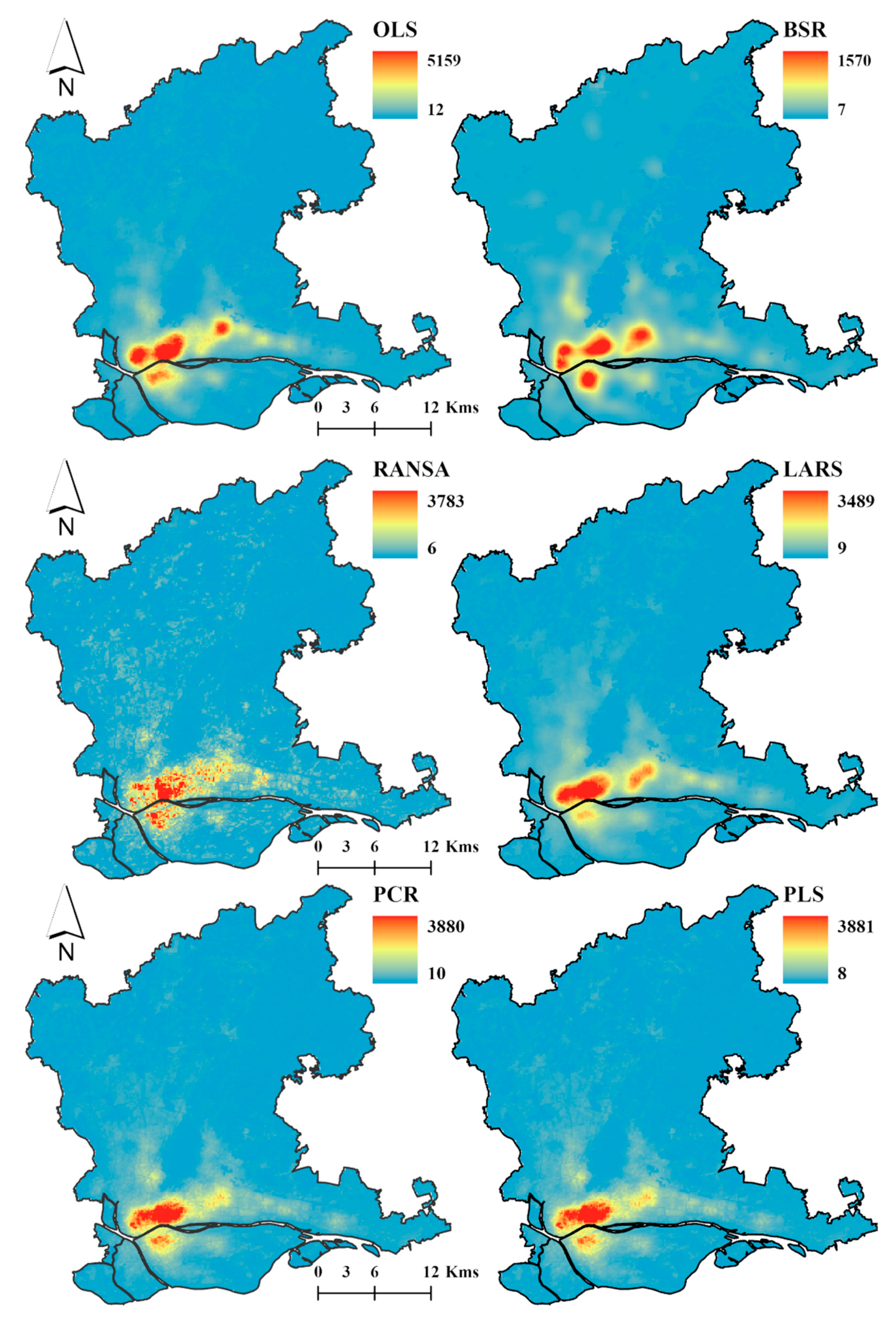
3.2. Spatial Decomposition Results Based on Different Regression Models

3.2.1. Model Training Results for Population Density Regression on Subdistrict Scale

As mentioned above, the population densities of all the subdistricts were taken as the dependent variables (Y), while the values of nineteen influence factors were selected as the independent variables (X). The twelve models were trained using the GridSearchCV function and ten-fold cross-validation. The model training results and fitted models are shown in

Table 5. Model training results through 10-fold cross-validation.

Algorithm	R2	RMSE	MAPE (%)	MABE
OLS	0.924	6471.913	48.063	4733.677
BSR	0.977	3547.13	34.667	2282.022
RANSAC	0.899	7421.336	59.307	5125.861
LARS	0.888	7838.545	69.02	5759.284
PCR	0.914	6868.028	102.96	6133.461
PLS	0.922	6535.272	89.433	5666.922
Lasso	0.924	6459.609	51.043	4819.67
Ridge	0.907	7128.09	76.27	5874.865
Elastic Net	0.915	6828.741	81.983	5814.385
SVR	0.876	8157.352	71.263	5924.128
KNN	0.925	6424.436	50.105	4711.419
RF	0.977	3606.155	21.562	2429.656

and

Table 6. Fitted models for population density regression in the subdistrict scale.

Algorithm	Regression Coefficients
OLS	Intercept: 1901.1, X18: −2701.682, X19: 3361.864, X14: −18,485.94, X16: −2380.934, X10: −64,862.639, X2: 41,694.214, X11: −4371.515, X13: −1373.629, X6: −11,883.214, X5: −5818.896, X7: 350.947, X3: 62,982.759, X9: 38,206.661, X8: 1205.293, X4: −5115.524, X1: 4267.389, X12: 8741.203, X17: 23,840.905, X20: 326.614
BSR	Intercept: −3403.922, X18: 5337.635, X19: −93,394.656, X14: 53,891.134, X16: 7504.77, X10: −25,863.081, X2: 86,852.708, X11: 20,344.519, X13: 21,736.836
LARS	Intercept: −2900.887, X18: 0.0, X19: 0.0, X14: 0.0, X16: 0.0, X10: 0.0, X2: 30,624.587, X11: 0.0, X13: 0.0, X6: 0.0, X5: 0.0, X7: 0.0, X3: 7234.966, X9: 0.0, X8: 0.0, X4: 0.0, X1: 42,087.766, X12: 0.0, X17: 8925.469, X20: 0.0
RANSAC	Intercept: 3153.065, X18: −2329.204, X19: −2244.842, X14: −15,134.735, X16: −680.564, X10: −68,444.646, X2: 62,309.348, X11: 8446.039, X13: −32,618.475, X6: −1115.962, X5: −70,222.187, X7: 1347.96, X3: 14,151.086, X9: 67,667.638, X8: 32,527.374, X4: 3245.049, X1: −9210.031, X12: 39,307.589, X17: 4264.226, X20: 6561.059
PCR	Intercept: 21,141.643, PCA_comp_1: 22,453.882, PCA_comp_2: 13,210.932, PCA_comp_3: 34,922.859, PCA_comp_4: 4447.51, PCA_comp_5: −18,119.79, PCA_comp_6: 21368.82
PLS	Intercept: 21,141.643, X18: 2373.471, X19: −2654.313, X14: −9015.102, X16: −448.029, X10: −8446.882, X2: 32,589.97, X11: −12,449.821, X13: −2399.885, X6: 3084.427, X5: −7366.366, X7: 10,634.243, X3: 21,308.299, X9: 48,67.91, X8: 6529.518, X4: 16,855.52, X1: 22,241.48, X12: −5143.745, X17: 18,142.841, X20: −7780.463
Lasso	Intercept: 1964.62, X19: −1589.42, X14: 192.919, X16: −17,277.211, X10: 0.0, X2: −42,274.926, X11: 39,859.867, X13: −6965.692, X6: 0.0, X5: 0.0, X7: −3148.53, X3: 0.0, X9: 53,982.023, X8: 18,387.694, X4: 0.0, X1: −1408.461, X12: 10,624.522, X17: 551.24
Ridge	Intercept: −564.43, X18: −463.238, X19: 6.035, X14: −11,254.556, X16: 294.123, X10: −12,849.21, X2: 27,474.343, X11: −10,941.451, X13: −971.068, X6: 3010.897, X5: −5240.741, X7: 8376.518, X3: 18,889.473, X9: 5893.067, X8: 9164.593, X4: 6572.182, X1: 29,686.551, X12: 1171.75, X17: 18,537.403, X20: −3996.295
Elastic Net	Intercept: −2646.624, X18: 75.337, X19: −523.813, X14: −6518.326, X16: 1903.378, X10: −3420.06, X2: 18,940.878, X11: −6626.514, X13: 1211.34, X6: 3634.379, X5: −2755.817, X7: 8352.229, X3: 13,091.079, X9: 5572.288, X8: 7356.989, X4: 11,183.943, X1: 23,092.917, X12: 655.476, X17: 14,025.249, X20: −2551.125
SVR	Non-parametric
KNN	Non-parametric
RF	Non-parametric

, respectively.

From Table 4 and Table 5, it can be seen that the models trained by the various algorithms presented obvious differences. When the RMSE metric is used as the only indicator to measure model accuracy, the BSR model is the best model, while the SVR model is the worst model. The results demonstrate that the BSR model can find the optimal estimator through loop traversal in theory. When the MAPE metric is used as the only indicator to measure model accuracy, the KNN model is the best model and the PCR model is the worst model. The models trained by the twelve algorithms are effective when the R² indicator is applied as the only metric for measuring the model’s performance. Generally speaking, when the accuracies of several models are relatively close, simple models should be given priority over complex models. Among the nine linear regression models, the LARS model is the simplest one, with only four independent variables. The PCR model is the second simplest model, with six independent variables. However, the interpretability of the PCR model is too weak.

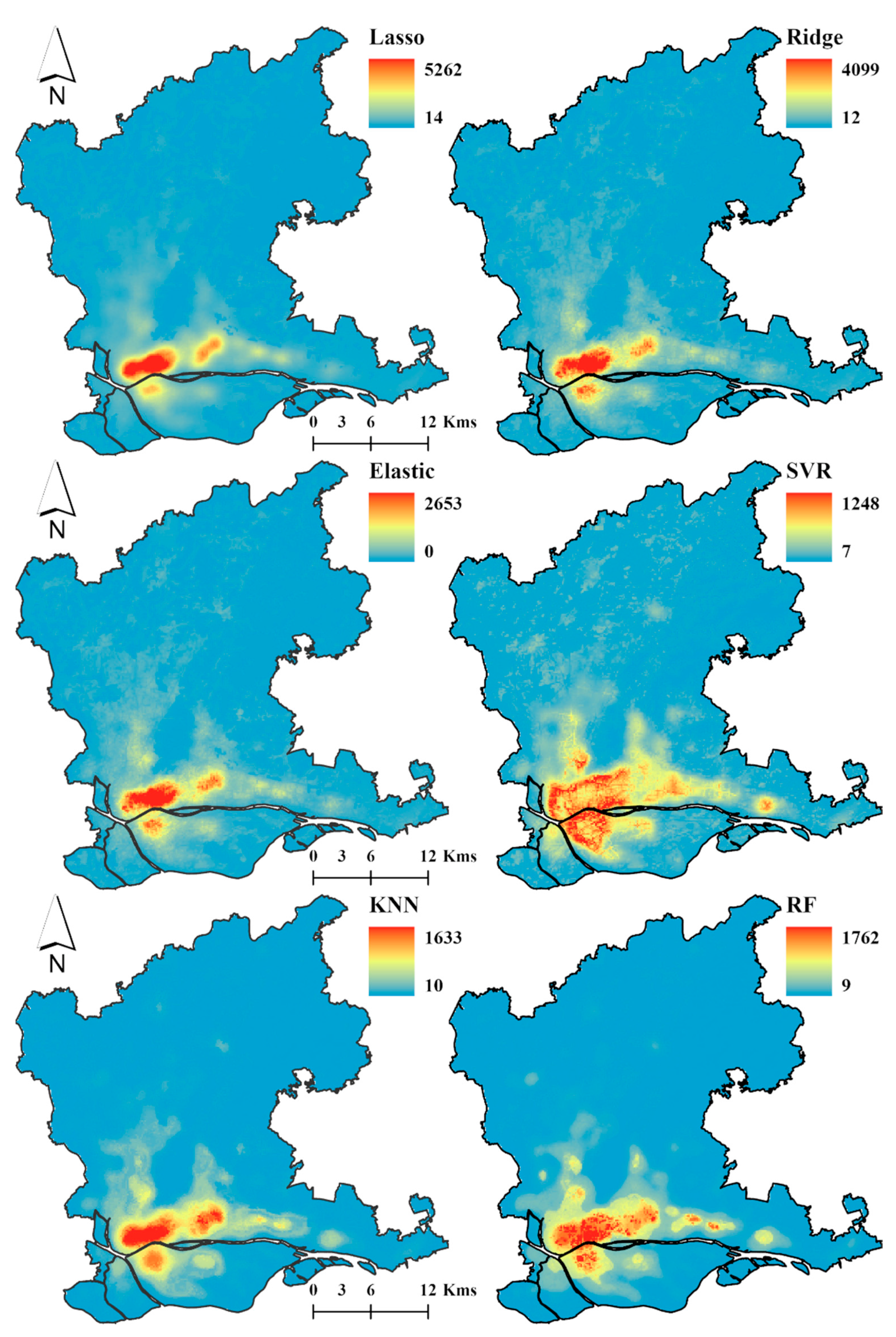
3.2.2. Spatial Decomposition Results of Demographic Data with Different Regression Models

The twelve trained models were applied to the test set to predict the population density in the grid scale. The spatial decomposition results of the demographic data generated by the twelve regression models are shown in Figure 3.

As can be observed in Figure 3, the distribution patterns of predicted populations derived from these twelve models were clearly different from each other. In general, all the spatial decomposition results reflected the pattern of population concentration in the central area. The most concentrated pattern was shown in the results from the BSR model. By contrast, the sparsest pattern was shown in the results of the SVR model. The highest predicted population of a cell was 5262, which appeared in the results from the Lasso model. The lowest predicted population of a cell was zero, which appeared in the results from the Elastic Net model. It is worth noting that, except for the Elastic Net model, there were no zero-valued grid cells in the decomposition results of the remain eleven algorithms. Among the results generated by the three nonlinear regression algorithms, the distribution of cells with high predicted populations were wider than those of the linear algorithms, especially the SVR model. According to the demographic data in the subdistrict scale, it seems that the nonlinear regression algorithms revealed the spatial heterogeneity of population distributions more clearly.

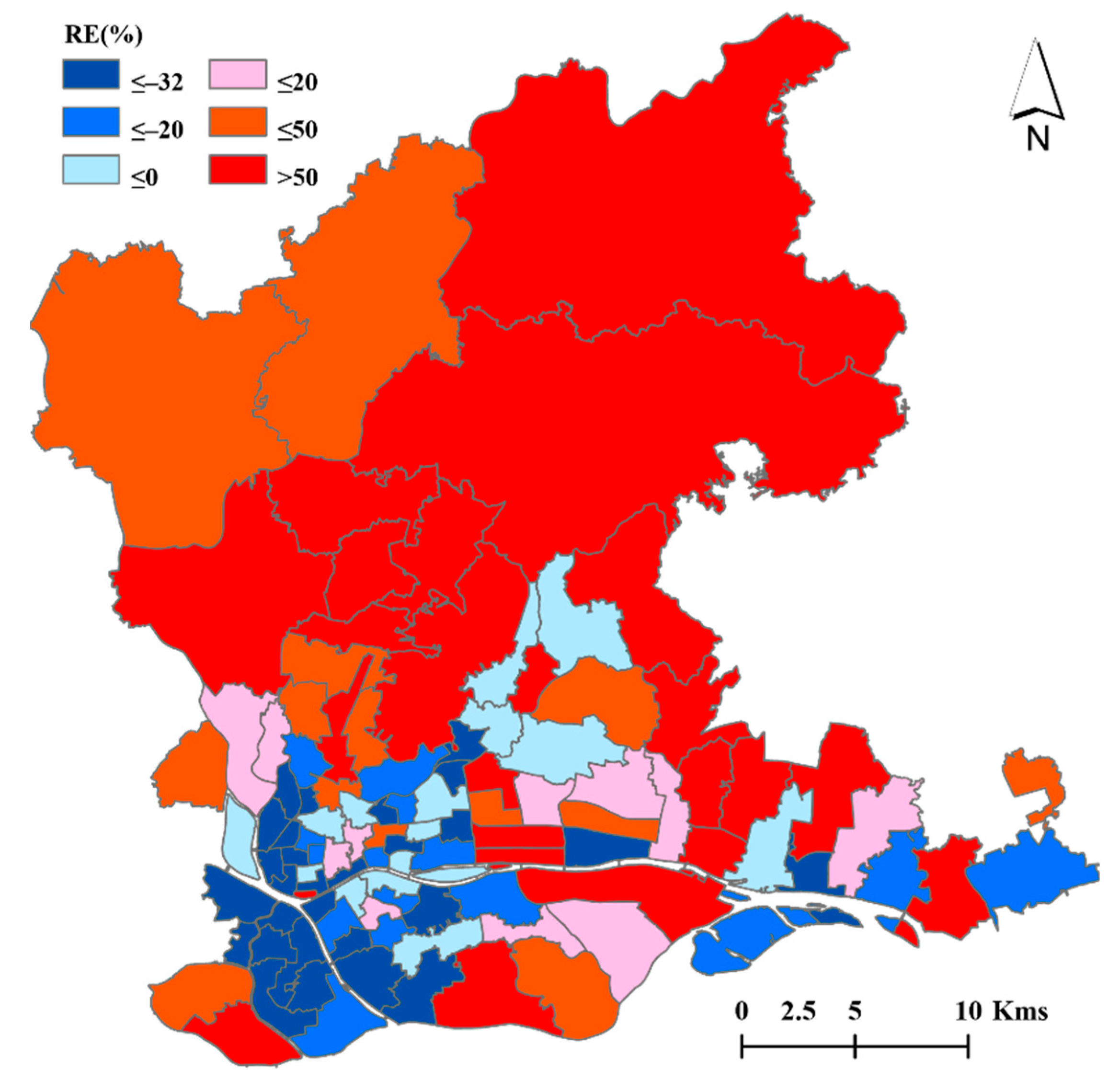
3.3. Accuracy Assessment of Spatial Decomposition Results Using Twelve Regression Models

The accuracy of the decomposition results derived from the various algorithms was evaluated using metrics such as RMSE, MAPE, and so on. The accuracy assessment of the spatial decomposition results derived from the twelve algorithms is shown in

Table 7. Evaluation of decomposition results.

Algorithms	R2	RMSE	MABE	MAPE (%)
OLS	0.924	6471.913	48.063	4733.677
BSR	0.977	3547.13	34.667	2282.022
RANSAC	0.899	7421.336	59.307	5125.861
LARS	0.888	7838.545	69.02	5759.284
PCR	0.914	6868.028	102.96	6133.461
PLS	0.922	6535.272	89.433	5666.922
Lasso	0.924	6459.609	51.043	4819.67
Ridge	0.907	7128.09	76.27	5874.865
Elastic Net	0.915	6828.741	81.983	5814.385
SVR	0.876	8157.352	71.263	5924.128
KNN	0.925	6424.436	50.105	4711.419
RF	0.977	3606.155	21.562	2429.656

.

We can see immediately from Table 7 that the decomposition accuracy of the OLS model was the worst as the RMSE value of the OLS model exceeded 200 and the R² value was only 0.19. Hence, an obvious inference is that the OLS model has an overfitting problem in our study case. Compared with the OLS model, the decomposition accuracies of the BSR model, the RANSAC model and the LARS model were significantly improved. The comparison results demonstrated that subsetting is an effective method to correct the overfitting problem. However, among the three subsetting regression models, the accuracy of the LARS model was the best, followed by the RANSAC model and the BSR model. This ranking implies that the solution to searching for the optimal subset combination through loop traversal may not necessarily lead to a better model. The decomposition results of four regularization models, Lasso, Ridge, Elastic Net, and B-Ridge, showed that regularization is also one of the general solutions to alleviate overfitting. In both the OLS model and the four regularization models, the decomposition accuracy was significantly improved.

Among the three regularized regression models, the ridge regression model demonstrated the best prediction accuracy. Therefore, we can speculate that L2 regularization was the optimal regularization scheme in our study. Compared with the OLS model, the decomposition accuracies of the PCR model and the PLS model were also significantly improved, indicating that the feature reduction method is also useful in alleviating overfitting. The prediction accuracies of the PCR model and the PLS model were very close; they can be considered as almost equivalent models in this case. Based on the accuracy evaluation results of the above nine linear regression models, it can be considered that in addition to the OLS regression model, the remaining linear regression models are also suitable for our study. Among the linear regression models, the ridge regression model was preferred as it demonstrated the best decomposition accuracy.

It is obvious that the prediction accuracies of three nonlinear regression models presented in Table 4 were significantly better than in the OLS model. The decomposition accuracies of the three nonlinear regression models, in ascending order, were the SVR model, the RF model, and the KNN model. Among them, the R² values of the RF model and the KNN model both exceeded 0.7, indicating that they both offer good decomposition effects. Therefore, the KNN model and the RF model were both suitable for this study. Because the decomposition accuracy of the RF model was slightly worse than that of the KNN model, the KNN model was the preferred nonlinear model in this study. The experiment demonstrated again that there is no universal model for machine learning regression. The statistics for the proportion of cell numbers in the twelve model outputs are shown in Figure 4.

Among the decomposition results generated by the twelve regression models, the proportion of cells with a population density of less than 17,000 people/km² exceeded 90% (see Figure 4). In the decomposition results from the BSR model, the proportion of cells with a population density of less than 17,000 people/km² was the highest, about 96.76%. In contrast, in the decomposition results from the RF model, the proportion of cells with a population density of less than 17,000 people/km² was close to 91.6%, which was the lowest.

The proportion of subdistricts with different relative errors in the twelve model results is shown in Figure 5. As can be seen in Figure 5, the proportions of subdistricts with different relative errors derived from the twelve models varied. Generally speaking, when the RE value of the model was in the range of −30% and 30%, it can be considered that the model prediction was sufficiently accurate. When the RE value of the model output was higher than 30%, it can be considered that the predicted population was overestimated. When the RE value of the model output was less than −30%, it can be considered that the predicted population was underestimated.

The proportion of subdistricts with RE between −30% and 30% in the model output can be used to evaluate how many subdistricts present reasonable accuracy. The number of subdistricts with RE between −30% and 30% in the RF model output was the highest (there were 53 subdistricts within the range) while that of the BSR model was the lowest (only 25 subdistricts fell within the range). When the relative error value of the model output was higher than 30%, it can be considered that the predicted value was overestimated. In the decomposition results from the OLS model, 68 subdistricts demonstrated a relative error value higher than 30%, which accounted for 64.1% of the total number of subdistricts. In addition, there were 61 subdistricts with a relative error higher than 30% in the decomposition results from the Lasso model, which accounted for 57.5% of the total number of subdistricts. This result implied that the OLS model and the Lasso model both displayed a serious tendency to overestimate the population density. It is worth mentioning that in the spatial decomposition results from the OLS model, the number of subdistricts with an RE greater than 30% accounted for more than 64%, which may be the main manifestation of the poor accuracy of the OLS model. In the decomposition results from the BSR model and the RANSAC model, the number of subdistricts with an RE higher than 30% were 28 and 29, respectively. Therefore, it can be considered that the BSR model and the RANSAC model were regression models with a lower tendency towards overestimation. The quantity of subdistricts with an RE of less than −30% in the decomposition results from the OLS model was 7, which was the lowest of all the models. In contrast, the number of subdistricts with an RE of less than −30% in the decomposition results from the BSR model was 53, which was the highest of all the models. These results may imply that the BSR model had a serious tendency towards underestimation. In summary, compared with that of the linear regression models, the accuracy of the non-linear regression models, RF, KNN, and SVR, was superior. Because the best performance was observed in the KNN model, the spatial decomposition results of the demographic data from the KNN algorithm are discussed in the following text. The gridded population map derived from the KNN model is shown in Figure 6 (overlayed by the boundary of subdistricts rendered with a light gray dotted line).

The population distribution in the study area presented an obvious spatial pattern: high in the center and low in the periphery (as seen in Figure 6). Specifically, the population density was highest in the northeast part of YueXiu district, LiWan district, and TianHe district. The cells with high population density were mainly distributed in the range of 5 km to the north of the Pearl River channel and 3 km to the south of the channel. The population in the northern part of the Pearl River channel was higher than that in the southern part of the Pearl River channel. It was demonstrated that the spatial pattern illustrated by the gridded population data was clearer than the demographic data. The relative error map of each subdistrict is illustrated in Figure 7 in order to evaluate the KNN model results at the subdistrict scale.

As can be seen from Figure 7, most of the populations of the subdistricts in LiWan district, YueXiu district, and the western part of HaiZhu district were underestimated. Meanwhile, most of the populations of the subdistricts in TianHe district, the northern part of HuangPu district, and the eastern part of HaiZhu District were overestimated. Specifically, the subdistricts with an RE greater than 50% included Taihe, Zhongluotan, Yongping, Junhe, Shijing, Songzhou, Jinsha, Tongde, Tangjing, Xinshi, Sanyuanli, Tonghe, Liuhua, Fenghuang, Yuangang, Changxing, Xintang, Huangcun, Zhuji, Qianjin, Dasha, Suidong, Huazhou, Nanzhou, Pazhou, Liede, Xiancun, and Linhe. The subdistricts with an RE lower than −32% included Changzhou, HuangPu, Shayuan, Nanshitou, Ruibao, Meihucun, Jianshe, Dadong, Nanhuaxi, Renmin, Zhanqian, Xicun, Nanyuan, Caihong, Changhua, Fengyuan, Duobao, Lingnan, ShiweiTang, Huadi, Dongjiao, Baihedong, and Dongsha. Based on the demographic data, it was found that the KNN algorithm generally underestimated populations in the subdistricts with higher population density, and overestimated them in the subdistricts with lower population density. Combined with the spatial pattern of the ancillary data, such as POI, night lights data, and so on, we found that in the areas where various modeling data were densely distributed, the prediction results of the KNN algorithm were mostly underestimations. On the contrary, in the area where the ancillary data were sparsely distributed, the prediction results of the KNN algorithm were mostly overestimations. A reasonable inference is that due to the fact that the differences in the socio-economic environment within the region were ignored, a single or global KNN model may have led to unreasonable estimations in the model output. According to previous studies, the zonal strategy can effectively solve the shortcomings of the global model by using secondary partition modeling [23,63]. Therefore, the zonal strategy should be given priority when dealing with the shortcomings of the global model.

4. Discussion and Conclusions

4.1. Discussion

In this study, we used twelve machine learning regression algorithms to spatially decompose demographic data into a grid scale by integrating geospatial data from various sources such as POI, night lights, land use, and so on. The following issues should be discussed further, based on the above experimental analysis.

4.1.1. Principal Findings and Meaningful Implication

(1)

The methodology framework proposed in this paper provides an effective and rapid approach to the fine spatial decomposition of demographic data. The auxiliary data from various sources can be combined for gridded population mapping via machine learning regression. It was demonstrated that location-based services (LBS) data, derived from mobile phones, Baidu map, Tencent LBS, Sina Weibo, and so on, offer the possibility of illustrating gridded population maps more accurately and finely in urban areas [11,22,64,65,66,67,68,69,70,71]. In particular, the accuracy of gridded population maps can be improved significantly through the integration of remote sensing data and LBS data [72]. The geographical detector model can quickly and effectively identify the factors influencing population density distributions. Three non-linear machine learning regression algorithms, including the SVR model, the RF model and the KNN model, were employed in the spatial decomposition of demographic data, which was demonstrated to be useful for mining implicit non-linear relationships. The proposed approach can provide very useful information to support future research on the spatial decomposition of demographic data with growing multi-source geospatial data [22,73].

(2)

The results of this study indicate that the OLS model is prone to overfitting in the spatial decomposition of demographic data. As we know, bias and variance are two key characteristics of estimators that must be considered in regression analysis; the former measures the accuracy of the model, while the latter measures the stability of the model. Clearly, ordinary least square linear regression is more affected by variance due to the excess of independent variables or collinearity. Both regularization and subsetting methods can effectively improve overfitting in the OLS model. Because all possible feature combinations are traversed, the features selected by the BSR model should, theoretically, offer an optimal combination. However, in this case, the improvement effect of the regularization methods on overfitting was better than in the BSR model, whether in the L1 regularization or the L2 regularization. These results again reflected the shortcomings of the BSR model. The reason why the BSR model is not the best in practical applications is still unclear; the unreasonable selection of independent variables, collinearity, and so on, are worth considering in this regard. In addition, another drawback of the BSR model is that it needs to fit 2^p models, which is very computationally expensive (assuming the model includes p features). For this reason, we believe that for the spatial decomposition of demographic data, the regularization method is better than the subsetting method in improving overfitting.

(3)

The results of our case study demonstrate that for the spatial decomposition of demographic data, nonlinear regression models offer greater accuracy than linear regression models. The results may imply that the relationship between population density distribution and impact factors is complicated and non-linear. Since the nonlinear regression model can deal better with the collinearity of independent variables and other problems that easily lead to overfitting, we suggest that when conducting research on the spatial decomposition of demographic data, priority should be given to using nonlinear regression models to improve the accuracy of results. However, the results of regression models such as the KNN model, the SVR model and the RF model are non-parametric, and the interpretability of these models is very poor. Therefore, when the interpretability of the model needs to be taken into account, linear regression models based on the regularization method should be given priority.

4.1.2. Explanations for Further Research

There are some limitations in this study. The first disadvantage of this paper is that whether the results of our study are valid in other regions is still in doubt. As the study area was the main developed area of Guangzhou city, the POI data were sufficient to support the implementation of the proposed method. However, the applicability of the multi-source geospatial data-driven method in other regions still needs to be studied, especially in non-urban areas, where auxiliary data are relatively sparse. Hence, the proposed method may be more suitable for developed areas with abundant geospatial data.

Second, the data sources for prompting the fine-scale spatial decomposition research need to be enriched. Dynamic geo-data, such as mobile phone communication data [74], social media check-in data [64,67,68], GPS trajectory data [66], and so on, can effectively improve the accuracy of the proposed approach and provide the spatial-temporal information on population distribution on the fine scale, which is very important for issues in urban governance, such as emergency management, public service facility configuration, and so on. In future research, we could focus on revealing the spatial-temporal dynamics of population distribution with more individual-scale trajectory data, such as mobile phone signaling data, non-floating bicycle trajectory data, online car trip hailing data, and so on.

Finally, although this article discusses twelve commonly used linear regression models and non-linear regression models that were used to perform the experiments, the popular neural network model was not involved. However, studies of the spatial decomposition of demographic data based on neural networks are relatively rare. These issues are worthy of further exploration.

4.2. Conclusions

This paper compares the use of twelve machine learning regression algorithms in gridded population mapping of Guangzhou city, China. Various spatial data (such as night light images, land use, POI, roads, and so on) from different sources are considered in the study. To evaluate the performance of the twelve regression algorithms, several metrics were involved in this study. The results indicate that the proposed method has great potential in fine-scale gridded population mapping. The conclusions can be summarized as follows.

(1)

The R² values of the twelve regression algorithms discussed in this paper varied between 0.193 and 0.758. It can be said that besides the OLS algorithm, all the algorithms produced acceptable decomposition results by taking the R² as the only evaluation metric. When all the algorithms were evaluated with the metric of MAPE, it was observed that the MAPE values of these models varied between 78.58% and 174.37%. That is, it can be concluded that all the decomposition results can be considered “reasonable”, apart from those of the OLS algorithm. Both the regularization method and the subsetting method can effectively alleviate overfitting in the OLS model. For the spatial decomposition of demographic data, the regularization method is better than the subsetting method in alleviating overfitting.

(2)

According to the model evaluation results, it can be seen that nonlinear regression algorithms offer greater accuracy than linear regression algorithms. Among the three nonlinear regression algorithms discussed in this study, the RF algorithm and the KNN algorithm both produced better results than the SVR algorithm, especially the KNN algorithm. Therefore, the KNN algorithm was recognized as a more suitable algorithm for this study. However, the accuracy of the KNN algorithm in other areas still needs to be evaluated. In addition, because the KNN algorithm does not provide a parameterized regression model, the interpretability of the decomposition model is very poor.

References

1. Azar, D.; Engstrom, R.; Graesser, J.; Comenetz, J. Generation of fine-scale population layers using multi-resolution satellite imagery and geospatial data. Remote Sens. Environ. 2013, 130, 219–232. [Google Scholar] [CrossRef]
2. Balk, D.L.; Deichmann, U.; Yetman, G.; Pozzi, F.; Hay, S.I.; Nelson, A. Determining Global Population Distribution: Methods, Applications and Data. In Advances in Parasitology; Hay, S.I., Graham, A., Rogers, D.J., Eds.; Academic Press: London, UK, 2006; Volume 62, pp. 119–156. [Google Scholar]
3. Weber, E.M.; Seaman, V.Y.; Stewart, R.N.; Bird, T.J.; Tatem, A.J.; McKee, J.J.; Bhaduri, B.L.; Moehl, J.J.; Reith, A.E. Census-independent population mapping in northern Nigeria. Remote Sens. Environ. 2018, 204, 786–798. [Google Scholar] [CrossRef]
4. O’neill, B.C.; Dalton, M.; Fuchs, R.; Jiang, L.; Pachauri, S.; Zigova, K. Global demographic trends and future carbon emissions. Proc. Natl. Acad. Sci. USA 2010, 107, 17521–17526. [Google Scholar] [CrossRef] [Green Version]
5. Wang, Y.; Huang, C.; Feng, Y.; Zhao, M.; Gu, J. Using Earth Observation for Monitoring SDG 11.3.1-Ratio of Land Consumption Rate to Population Growth Rate in Mainland China. Remote Sens. 2020, 12, 357. [Google Scholar] [CrossRef] [Green Version]
6. Tuholske, C.; Gaughan, A.E.; Sorichetta, A.; de Sherbinin, A.; Bucherie, A.; Hultquist, C.; Stevens, F.; Kruczkiewicz, A.; Huyck, C.; Yetman, G. Implications for Tracking SDG Indicator Metrics with Gridded Population Data. Sustainability 2021, 13, 7329. [Google Scholar] [CrossRef]
7. Gallopín, G.C. Human dimensions of global change: Linking the global and the local processes. Int. Soc. Sci. J. 1991, 43, 707. [Google Scholar]
8. Zhou, Y.; Ma, M.; Shi, K.; Peng, Z. Estimating and Interpreting Fine-Scale Gridded Population Using Random Forest Regression and Multisource Data. ISPRS Int. J. Geo-Inf. 2020, 9, 369. [Google Scholar] [CrossRef]
9. Wu, T.J.; Luo, J.C.; Dong, W.; Gao, L.J.; Hu, X.D.; Wu, Z.F.; Sun, Y.W.; Liu, J.S. Disaggregating County-Level Census Data for Population Mapping Using Residential Geo-Objects With Multisource Geo-Spatial Data. IEEE J. Sel. Top. Appl. Earth Obs. Remote Sens. 2020, 13, 1189–1205. [Google Scholar] [CrossRef]
10. Yao, Y.; Liu, X.; Li, X.; Zhang, J.; Liang, Z.; Mai, K.; Zhang, Y. Mapping fine-scale population distributions at the building level by integrating multisource geospatial big data. Int. J. Geogr. Inf. Sci. 2017, 31, 1220–1244. [Google Scholar] [CrossRef]
11. Deville, P.; Linard, C.; Martin, S.; Gilbert, M.; Stevens, F.R.; Gaughan, A.E.; Blondel, V.D.; Tatem, A.J. Dynamic population mapping using mobile phone data. Proc. Natl. Acad. Sci. USA 2014, 111, 15888–15893. [Google Scholar] [CrossRef] [Green Version]
12. Goodchild, M.F.; Anselin, L.; Deichmann, U. A Framework for the Areal Interpolation of Socioeconomic Data. Environ. Plan. A 1993, 25, 383–397. [Google Scholar] [CrossRef]
13. Tobler, W.; Deichmann, U.; Gottsegen, J.; Maloy, K. World population in a grid of spherical quadrilaterals. Int. J. Popul. Geogr. 1997, 3, 203–225. [Google Scholar] [CrossRef]
14. Lin, J.; Cromley, R.G. Evaluating geo-located Twitter data as a control layer for areal interpolation of population. Appl. Geogr. 2015, 58, 41–47. [Google Scholar] [CrossRef]
15. Shi, X.; Li, M.; Hunter, O.; Guetti, B.; Andrew, A.; Stommel, E.; Bradley, W.; Karagas, M. Estimation of environmental exposure: Interpolation, kernel density estimation or snapshotting. Ann. GIS 2019, 25, 1–8. [Google Scholar] [CrossRef] [Green Version]
16. Qiu, F.; Cromley, R. Areal Interpolation and Dasymetric Modeling. Geogr. Anal. 2013, 45, 213–215. [Google Scholar] [CrossRef]
17. Ye, T.; Zhao, N.; Yang, X.; Ouyang, Z.; Liu, X.; Chen, Q.; Hu, K.; Yue, W.; Qi, J.; Li, Z.; et al. Improved population mapping for China using remotely sensed and points-of-interest data within a random forests model. Sci. Total Environ. 2018, 658, 936–946. [Google Scholar] [CrossRef]
18. Xu, M.; Cao, C.; Jia, P. Mapping Fine-Scale Urban Spatial Population Distribution Based on High-Resolution Stereo Pair Images, Points of Interest, and Land Cover Data. Remote Sens. 2020, 12, 608. [Google Scholar] [CrossRef] [Green Version]
19. Balk, D.L.; Yetman, G. The Global Distribution of Population: Evaluating the Gains in Resolution Refinement; Columbia University: New York, NY, USA, 2004. [Google Scholar]
20. Dobson, J.E.; Bright, E.A.; Coleman, P.R.; Durfee, R.C.; Worley, B.A. A Global Population Database for Estimating Population at Risk. Photogramm. Eng. Remote Sens. 2000, 66, 849–858. [Google Scholar]
21. Freire, S.; Macmanus, K.; Pesaresi, M.; Doxsey-Whitfield, E.; Mills, J. Development of new open and free multi-temporal global population grids at 250 m resolution. In Proceedings of the Agile, Helsinki, Finland, 14–16 June 2016. [Google Scholar]
22. Stevens, F.R.; Gaughan, A.E.; Linard, C.; Tatem, A.J. Disaggregating Census Data for Population Mapping Using Random Forests with Remotely-Sensed and Ancillary Data. PLoS ONE 2015, 10, e0107042. [Google Scholar] [CrossRef] [Green Version]
23. Zhao, G.; Yang, M. Urban Population Distribution Mapping with Multisource Geospatial Data Based on Zonal Strategy. ISPRS Int. J. Geo-Inf. 2020, 9, 654. [Google Scholar] [CrossRef]
24. Thomson, D.R.; Gaughan, A.E.; Stevens, F.R.; Yetman, G.; Elias, P.; Chen, R. Evaluating the Accuracy of Gridded Population Estimates in Slums: A Case Study in Nigeria and Kenya. Urban Sci. 2021, 5, 48. [Google Scholar] [CrossRef]
25. Gaughan, A.E.; Stevens, F.R.; Catherine, L.; Peng, J.; Tatem, A.J.; Francesco, P. High Resolution Population Distribution Maps for Southeast Asia in 2010 and 2015. PLoS ONE 2013, 8, e55882. [Google Scholar] [CrossRef] [PubMed]
26. Azar, D.; Graesser, J.; Engstrom, R.; Comenetz, J.; Leddy, R.M., Jr.; Schechtman, N.; Andrews, T. Spatial refinement of census population distribution using remotely sensed estimates of impervious surfaces in Haiti. Int. J. Remote Sens. 2010, 31, 5635–5655. [Google Scholar] [CrossRef]
27. Hastie, T.; Tibshirani, R.; Tibshirani, R. Best Subset, Forward Stepwise or Lasso? Analysis and Recommendations Based on Extensive Comparisons. Stat. Sci. 2020, 35, 579–592. [Google Scholar] [CrossRef]
28. Hocking, R.R.; Leslie, R.N. Selection of the Best Subset in Regression Analysis. Technometrics 1967, 9, 531–540. [Google Scholar] [CrossRef]
29. Beale, E.M.L.; Kendall, M.G.; Mann, D.W. The Discarding of Variables in Multivariate Analysis. Biometrika 1967, 54, 357–366. [Google Scholar] [CrossRef]
30. Efron, B.; Hastie, T.; Johnstone, I.; Tibshirani, R. Least angle regression. Ann. Stat. 2004, 32, 407–499. [Google Scholar] [CrossRef] [Green Version]
31. Tibshirani, R. Regression Shrinkage and Selection via the Lasso. J. R. Stat. Soc. Ser. B (Methodol.) 1996, 58, 267–288. [Google Scholar] [CrossRef]
32. Chen, S.S.; Donoho, D.L.; Saunders, M.A. Atomic Decomposition by Basis Pursuit. SIAM J. Sci. Comput. 1998, 20, 33–61. [Google Scholar] [CrossRef]
33. Marquardt, D.W.; Snee, R.D. Ridge Regression in Practice. Am. Stat. 1975, 29, 3–20. [Google Scholar] [CrossRef]
34. Dorugade, A.V.; Kashid, D.N. Alternative Method for Choosing Ridge Parameter for Regression. Appl. Math. Sci. 2010, 4, 447–456. [Google Scholar]
35. Hans, C. Elastic Net Regression Modeling With the Orthant Normal Prior. J. Am. Stat. Assoc. 2011, 106, 1383–1393. [Google Scholar] [CrossRef]
36. Zou, H.; Zhang, H.H. On the Adaptive Elastic-Net with a Diverging Number of Parameters. Ann. Stat. 2009, 37, 1733–1751. [Google Scholar] [CrossRef] [PubMed] [Green Version]
37. Zou, H.; Hastie, T. Regularization and Variable Selection via the Elastic Net. J. R. Stat. Soc. Ser. B (Stat. Methodol.) 2005, 67, 301–320. [Google Scholar] [CrossRef] [Green Version]
38. Mansfield, E.R.; Webster, J.T.; Gunst, R.F. An Analytic Variable Selection Technique for Principal Component Regression. J. R. Stat. Soc. Ser. C (Appl. Stat.) 1977, 26, 34–40. [Google Scholar] [CrossRef]
39. Greenberg, E. Minimum Variance Properties of Principal Component Regression. J. Am. Stat. Assoc. 1975, 70, 194–197. [Google Scholar] [CrossRef]
40. Reiss, P.T.; Ogden, R.T. Functional Principal Component Regression and Functional Partial Least Squares. J. Am. Stat. Assoc. 2007, 102, 984–996. [Google Scholar] [CrossRef]
41. Kaspi, O.; Yosipof, A.; Senderowitz, H. RANdom SAmple Consensus (RANSAC) algorithm for material-informatics: Application to photovoltaic solar cells. J. Cheminform. 2017, 9, 34. [Google Scholar] [CrossRef] [PubMed]
42. Fischler, M.A.; Bolles, R.C. Random sample consensus: A paradigm for model fitting with applications to image analysis and automated cartography. Commun. ACM 1981, 24, 381–395. [Google Scholar] [CrossRef]
43. Wang, L.Y.; Fan, H.; Wang, Y.K. Improving population mapping using Luojia 1-01 nighttime light image and location-based social media data. Sci. Total Environ. 2020, 730, 139148. [Google Scholar] [CrossRef] [PubMed]
44. Wang, J.F.; Li, X.H.; Christakos, G.; Liao, Y.L.; Zhang, T.; Gu, X.; Zheng, X.Y. Geographical Detectors-Based Health Risk Assessment and its Application in the Neural Tube Defects Study of the Heshun Region, China. Int. J. Geogr. Inf. Sci. 2010, 24, 107–127. [Google Scholar] [CrossRef]
45. Wang, J.; Xu, C. Geodetector: Principle and prospective. Acta Geogr. Sin. 2017, 72, 116–134. (In Chinese) [Google Scholar] [CrossRef]
46. Swami, A.; Jain, R. Scikit-learn: Machine Learning in Python. J. Mach. Learn. Res. 2013, 12, 2825–2830. [Google Scholar]
47. Oh, Y.J.; Park, H.S.; Min, Y. Understanding Location-Based Service Application Connectedness: Model Development and Cross-Validation. Comput. Hum. Behav. 2019, 94, 82–91. [Google Scholar] [CrossRef]
48. Gholinejad, S.; Naeini, A.A.; Amiri-Simkooei, A.R. Robust Particle Swarm Optimization of RFMs for High-Resolution Satellite Images Based on K-Fold Cross-Validation. IEEE J. Sel. Top. Appl. Earth Obs. Remote Sens. 2019, 12, 2594–2599. [Google Scholar] [CrossRef]
49. Park, H.; Kim, N.; Lee, J. Parametric models and non-parametric machine learning models for predicting option prices: Empirical comparison study over KOSPI 200 Index options. Expert Syst. Appl. 2014, 41, 5227–5237. [Google Scholar] [CrossRef]
50. Chunhua, Z.; Yingjie, T.; Naiyang, D. The new interpretation of support vector machines on statistical learning theory. Sci. China Math. 2010, 53, 151–164. [Google Scholar]
51. Onel, M.; Kieslich, C.A.; Guzman, Y.A.; Floudas, C.A.; Pistikopoulos, E.N. Big Data Approach to Batch Process Monitoring: Simultaneous Fault Detection and Diagnosis Using Nonlinear Support Vector Machine-based Feature Selection. Comput. Chem. Eng. 2018, 115, 503–520. [Google Scholar] [CrossRef]
52. Baseer, M.A.; Saidur, R. Application of support vector machine models for forecasting solar and wind energy resources: A review. J. Clean. Prod. 2018, 199, 272–285. [Google Scholar]
53. Chapelle, O.; Vapnik, V.; Bousquet, O.; Mukherjee, S. Choosing Multiple Parameters for Support Vector Machines. Mach. Learn. 2001, 46, 131–159. [Google Scholar] [CrossRef]
54. Hu, L.Y.; Huang, M.W.; Ke, S.W.; Tsai, C.F. The distance function effect on k-nearest neighbor classification for medical datasets. SpringerPlus 2016, 5, 1–9. [Google Scholar] [CrossRef] [PubMed] [Green Version]
55. Chen, H.L.; Huang, C.C.; Yu, X.G.; Xu, X.; Sun, X.; Wang, G.; Wang, S.J. An efficient diagnosis system for detection of Parkinson’s disease using fuzzy k-nearest neighbor approach. Expert Syst. Appl. 2013, 40, 263–271. [Google Scholar] [CrossRef]
56. Rodrigues, E.O. Combining Minkowski and Cheyshev: New Distance Proposal and Survey of Distance Metrics Using k-Nearest Neighbours Classifier. Pattern Recognit. Lett. 2018, 110, 66–71. [Google Scholar] [CrossRef]
57. Breiman, L. Random Forests. Mach. Learn. 2001, 45, 5–32. [Google Scholar] [CrossRef] [Green Version]
58. Yang, L.; Cao, Q.; Yu, Y.; Liu, Y. Comparison of daily diffuse radiation models in regions of China without solar radiation measurement. Energy 2020, 191, 116571. [Google Scholar] [CrossRef]
59. Rehman, S. Solar radiation over Saudi Arabia and comparisons with empirical models. Energy 1998, 23, 1077–1082. [Google Scholar] [CrossRef]
60. Zang, H.; Cheng, L.; Ding, T.; Cheung, K.W.; Wang, M.; Wei, Z.; Sun, G. Application of functional deep belief network for estimating daily global solar radiation: A case study in China. Energy 2020, 191, 116502. [Google Scholar] [CrossRef]
61. Ceylan, İ.; Gürel, A.E.; Ergün, A. The mathematical modeling of concentrated photovoltaic module temperature. Int. J. Hydrogen Energy 2017, 42, 19641–19653. [Google Scholar] [CrossRef]
62. Gouda, S.G.; Hussein, Z.; Luo, S.; Yuan, Q. Model selection for accurate daily global solar radiation prediction in China. J. Clean. Prod. 2019, 221, 132–144. [Google Scholar] [CrossRef]
63. Zhuo, L.; Ichinose, T.; Zheng, J.; Chen, J.; Shi, P.J.; Li, X. Modelling the population density of China at the pixel level based on DMSP/OLS non-radiance-calibrated night-time light images. Int. J. Remote Sens. 2009, 30, 1003–1018. [Google Scholar] [CrossRef]
64. Patel, N.N.; Stevens, F.R.; Huang, Z.; Gaughan, A.E.; Elyazar, I.; Tatem, A.J. Improving Large Area Population Mapping Using Geotweet Densities. Trans. GIS 2017, 21, 317. [Google Scholar] [CrossRef]
65. Bakillah, M.; Liang, S.; Mobasheri, A.; Arsanjani, J.J.; Zipf, A. Fine-resolution population mapping using OpenStreetMap points-of-interest. Int. J. Geogr. Inf. Syst. 2014, 28, 1940–1963. [Google Scholar] [CrossRef]
66. Zhao, X.; Zhou, Y.; Chen, W.; Li, X.; Li, X.; Li, D. Mapping hourly population dynamics using remotely sensed and geospatial data: A case study in Beijing, China. GISci. Remote Sens. 2021, 58, 717–732. [Google Scholar] [CrossRef]
67. Xu, Y.; Song, Y.; Cai, J.; Zhu, H. Population mapping in China with Tencent social user and remote sensing data. Appl. Geogr. 2021, 130, 102450. [Google Scholar] [CrossRef]
68. Miao, R.; Wang, Y.; Li, S. Analyzing Urban Spatial Patterns and Functional Zones Using Sina Weibo POI Data: A Case Study of Beijing. Sustainability 2021, 13, 647. [Google Scholar] [CrossRef]
69. Shang, S.; Du, S.; Du, S.; Zhu, S. Estimating building-scale population using multi-source spatial data. Cities 2021, 111, 103002. [Google Scholar] [CrossRef]
70. Nong, D.H.; Fox, J.M.; Saksena, S.; Lepczyk, C.A. The Use of Spatial Metrics and Population Data in Mapping the Rural-Urban Transition and Exploring Models of Urban Growth in Hanoi, Vietnam. Environ. Urban Asia 2021, 12, 156–168. [Google Scholar] [CrossRef]
71. Liu, J.; Ma, X.; Zhu, Y.; Li, J.; He, Z.; Ye, S. Generating and Visualizing Spatially Disaggregated Synthetic Population Using a Web-Based Geospatial Service. Sustainability 2021, 13, 1587. [Google Scholar] [CrossRef]
72. Yang, X.; Ye, T.; Zhao, N.; Chen, Q.; Yue, W.; Qi, J.; Zeng, B.; Jia, P. Population Mapping with Multisensor Remote Sensing Images and Point-Of-Interest Data. Remote Sens. 2019, 11, 574. [Google Scholar] [CrossRef] [Green Version]
73. Wardrop, N.A.; Jochem, W.C.; Bird, T.J.; Chamberlain, H.R.; Clarke, D.; Kerr, D.; Bengtsson, L.; Juran, S.; Seaman, V.; Tatem, A.J. Spatially disaggregated population estimates in the absence of national population and housing census data. Proc. Natl. Acad. Sci. USA 2018, 115, 3529–3537. [Google Scholar] [CrossRef] [Green Version]
74. Kang, C.; Liu, Y.; Ma, X.; Wu, L. Towards Estimating Urban Population Distributions from Mobile Call Data. J. Urban Technol. 2012, 19, 3–21. [Google Scholar] [CrossRef]
Figure 1. Map of the study area in Guangzhou, China.
Applsci 11 09424 g001
Figure 2. Technology roadmap.
Applsci 11 09424 g002
Figure 3. Gridded population maps derived from twelve regression models.
Applsci 11 09424 g003aApplsci 11 09424 g003b
Figure 4. Grouping statistics for the proportion of cells with different population densities.
Applsci 11 09424 g004
Figure 5. Grouping statistics for the proportion of subdistricts with different relative errors.
Applsci 11 09424 g005
Figure 6. Gridded population map derived from the KNN model.
Applsci 11 09424 g006
Figure 7. The relative error map of the KNN model.
Applsci 11 09424 g007