Abstract
A landslide inventory, after an intense rainfall event in 1998, Southwestern Korea, was collected by digitizing aerial photographs. This left high uncertainty in the inventoried features to be verified by ground truths. To reduce the uncertainty, the photographs were reexamined, supported by the time slider in Google Earth. We observed 77 deformed slopes, which were similar in shape and texture, to the inventoried landslides. We then sought to label the observed formations based on their spatial relationship with surrounding conditions. A three-phase methodology was developed. First, an inventory of landslide, no landslide, vulnerable slopes, and unlabeled features was analyzed based on spatial cluster patterns, and then the dimension was reduced using the t-distributed stochastic neighbor embedding (t-SNE). Second, the Apriori algorithm, based on association rule mining, was used to identify common relations in the inventory using landslide antecedent factors (derived from topographic and landcover maps) that are linked to areas of unlabeled features. Third, the findings were validated using Landsat TM (Thematic mapper) and ETM+(Enhanced thematic mapper) images acquired before and after the original inventory. Current research offers practical and economical solutions (reduced reliance on paid remote sensing sensors and field survey) to labeling and classification of missing or outdated spatial attributed information.
1. Introduction
Complete records of previous slope failures, their distribution, and slope condition, are among the best data for predicting the location of future failures. However, the inventory record needs, to the extent possible, to include complete and specific information on triggering factors, amount, type, area, volume, and date of incidents [1]. Slope activities, in any specific study area, have unique type and spatial distribution patterns that are determined by the prevailing antecedent (conditioning) factors. Specifically, the distribution of shallow landslides, a typical land degradation, tends to be spatially clustered and to reflect the distribution and structure of the slope material [2,3,4]. Topographic factors, such as slope condition, vegetation cover, soil type, and other land covers, tend to have classes or values common to each specific landslide type. Knowledge of the specific slope formation conditions at incident locations allows identification, and spatial classification of (previously unlabeled) slope formations with similar values of the antecedent factors.
To achieve such spatial pattern visualization, dimensionality reduction machine learning, with a t-distributed stochastic neighbor embedding (t-SNE) algorithm, offers a promising and practical capacity to analyze the structure of unlabeled slopes, leading to pattern identification and matching to known locations with similar formations [5]. t-SNE has been used to visualize high-dimensional datasets, such as remote sensing products and open data, by the clustered embedding of high-dimensional data into lower-dimensional space, such as a two- or three-dimensional map [6,7,8]. In addition, t-SNE is regarded as a very efficient technique for detecting potential errors in a reference dataset through visual analysis of a t-SNE plot [9]. Moreover, t-SNE returns highly compressed data, making it suitable for identification of large margins within a dataset. However, t-SNE may be unsuitable for datasets with recurring step-like temporal profiles [6].
The Apriori algorithm, based on association rule learning (ARL), is often used to identify frequently occurring item sets (associations) within a dataset [10]. It operates on large databases through several iterations based on a priori knowledge [11]. The Apriori algorithm has been widely employed to determine association rules in nonlinear modeling problems, and successfully applied to not only determine states of landslide deformation but also predict landslide movements [12,13]. Use of machine learning to assess associations among antecedents has become user friendly, especially with the adoption of the simple, but effective, Apriori association rules function.
To verify associations between landslide locations, we need evidence of actual conditions based on prior images or supporting reports. Semiautomatic techniques, including supervised classification-based change detection and manual digitization, may be used to extract landslides from satellite images [7]. More effective, in terms of time and effort, is the automatic detection of landslides from satellite images using unsupervised classification-based change detection [8]. Yang et al. [8] developed an automatic technique to detect landslide scars in the Jinsha River area of China. The developed technique was based on k-means classification of the Normalized Difference Vegetation Index (NDVI) time series derived from Sentinel-2 data. Wright and van Schaik [9] reported that variations in vegetation phenology over time affect the spectral responses of vegetation in tropical seasonal biomes, which can affect change detection applications. By contrast, Aydda et al. [14] confirmed that lithology change detection can be useful for identification of eroded areas. Therefore, in this study, a new automatic technique, based on lithology change detection, was used to detect landslides that occurred during/after intense rainfall events in Pohang state, Southwestern Korea.
Two machine learning algorithms and an automatic remote sensing extraction technique were used to label and classify additional spatial data, and provide missing attribute information, to complement the existing incomplete 1998 landslide inventory.
2. Study Area
The geology of the study area is predominantly Mesozoic Cretaceous sedimentary formations infiltrated by igneous (including volcanic) rocks, with further sedimentary and igneous rocks from the Cenozoic Tertiary [15]. Most landslides occurred in areas of tertiary sedimentary rock, mainly easily weathered mudstone and shale that make ground conditions vulnerable to landslides.
In 1998, landslides occurred in response to heavy rainfall of 150 mm over two days (25–26 July). After the rainfall event, a field reconnaissance survey was conducted in the Pohang area, using a 1:50,000 topographic map, and 297, mostly transitional, landslide locations were confirmed (258 of the landslides occurred in the Yeonil Formation surrounding the southern urban area and the coastal Duho Formation). A further 14 landslides were traced by the National Geographic Information Institute (https://www.ngii.go.kr/kor/main.do) through the analysis of 1:20,000 scale aerial photographs (taken between 4 June 1996 and 14 December 2004). In addition, in the same year, field investigations confirmed 21 no-landslide locations, representing safe slopes (Figure 1).
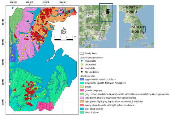
Figure 1.
Study area.
More recently, a field survey was conducted to find out if there are vulnerable or deformed slopes that might be susceptible to landslide creep. GPS-based surveys from 2015 to 2020 provided information about locations where significant signs of deformation were observed, such as tensile cracks, differential movement, continuous soil leakage, and bending trees. A total of 20 vulnerable points were assessed. These included locations of verified slope creep (8) identified by Park et al. [16], an additional point added by updated field report, and 11 points with continuous soil leakage and curved trees. Some of these have ground cracks or subsidence, and others have cracks in buildings and retaining walls, caused by an earthquake of magnitude 5.4 that occurred on 15 November 2017.
The 1:20,000 scale aerial photographs were examined, in conjunction with time-slider Google Earth images, and 73 locations, with similarly eroded landcover as in the 1998 inventory, were observed. It could not be determined with certainty whether these were areas of the landslide because of the small study area and thick green cover. Therefore, these locations were recorded as “unlabeled” landslide data. In Figure 1, we show a sample of the mentioned unlabeled features (Figure 2).
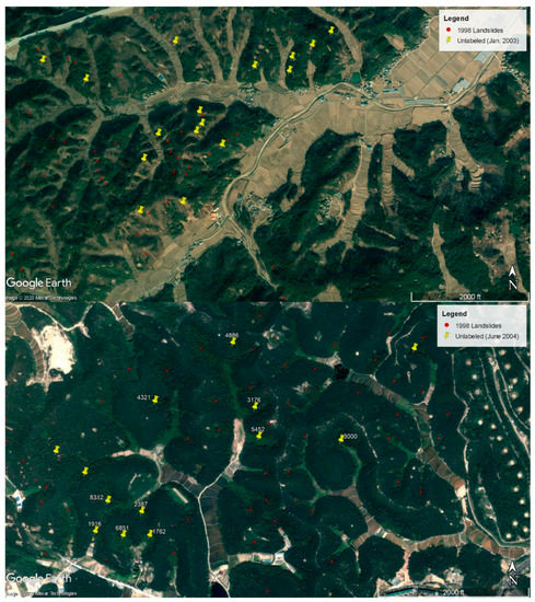
Figure 2.
Google earth images in January 2003 and June 2004.
3. Methodology
The nature of slope failure processes is dependent on the layers underneath and surrounding anthropogenic actions. Therefore, understanding of interdependencies among slope failure conditions (landslide, no landslide, or vulnerable slope) may contribute to a better understanding of patterns in newly collected data. In this research, unlabeled landslides, previously undocumented incidents observed in optical remote sensing images, were assumed to have occurred in July 1998 or later. The methodology, therefore, had three main components: (1) spatial pattern identification from slope formation inventory (20 vulnerable slopes, 73 unlabeled, 289 landslides, and 21 no landslides) using t-SNE cluster analysis; (2) identification of conditioning factor dependencies using data mining association rules; and (3) validation using temporal changes in Landsat processed data (Figure 3).
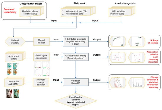
Figure 3.
Research methodology flowchart.
3.1. t-Distributed Stochastic Neighbor Embedding
t-SNE is a nonlinear machine learning dimensionality reduction algorithm. High-dimensional data are converted into two or three dimensions appropriate for scatter plotting [17]. The objective is to preserve as much of the significant structure of the high-dimensional data as possible in the low-dimensional map. Different transformations are applied in different regions such as to keep data points that are similar on a low-dimensional manifold closer together, rather than keeping dissimilar data points apart as in linear methods, such as principal component analysis (PCA).
A second interesting feature of t-SNE is a tunable parameter, called perplexity, which balances attention between local and global aspects of data and has a complex effect on the resulting distributions. The parameter can be used to predict the number of close neighbors each point has.
SNE calculations use Gaussian (normal) distributions and a gradient descent cost function that minimizes Kullback–Leibler divergence. While t-SNE calculations are very similar, they use Student’s t-distribution to recreate the probability distribution in lower-dimensional space [17]. The two steps of the t-SNE approach are as follows: First, create a probability distribution defining the relationships between data points in k-dimensional (high-dimensional) space; second, create a probability distribution defining the relationships between data counterparts in lower-dimensional space using Gaussian (normal) distributions.
Step 1: Conditional probability in high-dimensional space. This step determines the conditional probabilities defining potential neighbors or similarity between two points in k-dimensional space using Gaussian (normal) distributions as follows:
If we consider two points (xi and xj) chosen randomly from the dataset, the probability of xi picking xj as its neighbor or according to similarity is pj|i, which is proportional to the probability density under a Gaussian (normal) distribution centered at xi with variance σi.
The model calculates the conditional probability for all pairs of points in the dataset. If two points are very close to each other, the value of pj|i will be high (meaning that points are similar to each other), and if the points are far from each other, the value of pj|i will be small (meaning that points are dissimilar to each other).
Step 2: Conditional probability in low-dimensional space. This step finds the counterparts of similar points (xi and xj) in the lower-dimensional space using a Gaussian (normal) distribution.
If we considered yi and yj as the lower-dimensional counterparts of the points xi and xj, respectively, the conditional probability (qj|i) for yj being similar to yi is shown as follows:
The choice of cost function parameters in t-SNE is based on pure intuition and rule of thumb as t-SNE does not have a solid mathematical basis. For example, perplexity represents the perplexity of the conditional probability distribution induced by a Gaussian kernel, the recommended value is N1/2 (where N = number of attributes or samples) and is typically between 5 and 50. The number of principal components to keep can be found through randomization of the expression matrix, while the number of iterations is simply based on the rule the more iterations the better. When the algorithm reaches convergence, a further increase in the number of iterations will only marginally change the plot and will not enhance the results significantly.
3.2. Association Rule Learning
Apriori algorithms, as applied to data mining machine learning [18], use frequent itemset mining and ARL over databases [19]. The Apriori algorithm identifies frequently occurring patterns, and highlights general trends, in data. From these, three commonly used measures of association can be estimated.
- First-item support: an indication of how frequently an itemset appears in the dataset. It is the number of records containing the itemset divided by the total number of records in the database.
- Confidence: the support count of x U y (i.e., the number of times “x” and “y” occur together) divided by the support count of “x.”
- Lift: the observed support relative to the support expected if “x” and “y” were independent. It is calculated as the support count of x U y divided by the product of individual support counts of “x” and “y” support the count of x U y divided by the product of individual support counts of “x” and “y.”
The Apriori algorithm employs a level-wise search for frequent itemsets. It proceeds by identifying frequent individual items in the database and extending them to larger and larger itemsets, as long as those itemsets appear sufficiently often in the database [13]. For more information about the Apriori algorithms, see [20].
In the R environment, a seed was assigned, and the Rtsne function in the Rtsne package (T-Distributed Stochastic Neighbor Embedding using a Barnes–Hut Implementation) (https://cran.r-project.org/web/packages/Rtsne/) was run with optimizing the other parameters, including steps and perplexity. Different parameter values were run in a loop function to search for an optimum solution that easily differentiated between the different entities. Increasing steps (after a certain amount), which consumes more time and processing resources, does not significantly improve the results. By contrast, optimization of the perplexity value is highly recommended in such analysis, especially in the case of a complex distribution of features.
In preparation for the second phase, a data frame table was generated that included the target labels with the corresponding values for each thematic map. Eight thematic map layers, well cited and recommended as common conditioning factors of occurrence of landslide incidents, were derived from topographic, soil, and land cover maps and from Landsat 8 imagery. Elevation, slope angle, topographic wetness index (TWI), NDVI, tree age, soil depth, soil permeability index, and distance to drains were stacked and resampled to a common resolution (Figure 4).
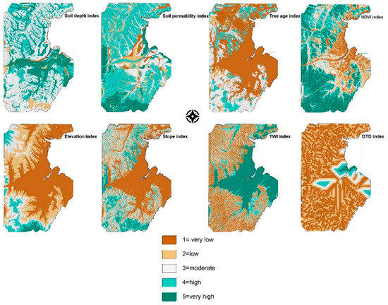
Figure 4.
Conditioning factors used in generating Apriori association rule table.
To run the Apriori analysis, we first preprocessed the input data to aid interpretation of the association rules.
- Consistent classification: a fixed number of classes for each thematic map. All the continuous data were converted into a categorical data structure. The potential classification methods (equal interval, natural break, standard deviation, and quantile) are appropriate for different data structures and applications. In landslide research, natural breaks, which preserve the natural distribution of the histogram, including real steps or changes, are commonly used [21]. Jenks Natural Breaks (Fisher–Jenks optimization algorithm) in the R classInt package (https://github.com/r-spatial/classInt/) was used to classify the continuous data into five index classes (for consistency with other naturally categorized maps).
- Normalization of the classification with meaningful names, i.e., convert the integer values to ordinal listings. We used 5–1, representing very high, high, moderate, low, and very low values.
The targeted landslide inventory (vulnerable slopes, no slide, unlabeled, and active landslides) data were collected from different sources, with different scales and feature representations (points and polygons). In order to reduce locational error, a polygon of 30 m diameter was generated for each point in the inventory (represent the average to maximum width of landslide incidents in the study area), and then 10 points were randomly generated inside each polygon. This increased the likelihood, as much as possible, that the centers of slopes and the exact locations of landslides were included in the dataset.
The derived inventory, stored in a single data frame with normalized values for each of the thematic maps, was sorted, and missing data were removed. Using the Apriori function in the R Arules package, Mining Association Rules and Frequent Itemsets (https://cran.r-project.org/package=arules), the association analysis was performed, and the association rules of each class of conditioning factors in the inventory were extracted.
For better control of the results, in terms of consistency, accuracy, length of rules, and rule-friendly interpretation, the function parameters including minimum length of rules (minlen), maximum length of rules (maxlen), support (supp), and confidence (conf) were fixed for all classes.
3.3. Lnadslides Inventory Validation
Two Landsat level 1 image scenes (geometrically corrected and radiometrically calibrated), acquired on 20 May 1998 and 22 October 1999 by the Landsat TM and Landsat ETM+ sensors (Figure 5), were processed as follows.
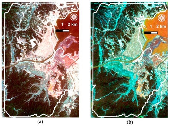
Figure 5.
(a) 20 May 1998 by Landsat TM sensors (b) 22 October 1999 by Landsat ETM+ Sensors.
- A dark object subtraction algorithm was used to correct atmospheric effects on the multispectral bands.
- Inversion of principal component bands, produced by PCA, was used to reduce noise.
- The ETM+ panchromatic band (15 m) was used to enhance the spatial resolution of the ETM+ multispectral bands.
- As landslides occurred on terrain contain clays (mud rocks) [22], band ratio 7/5 was applied to distinguish argillic from nonargillic materials [23].
- A map of change was created, from both band ratios, using image differencing change detection.
- The resultant change maps were classified using the IsoData algorithm, which is more efficient than other unsupervised classification algorithms (k-means and Expectation Maximization) for automatic extraction of objects from multispectral data [24].
Finally, we masked areas that were not of interest in the analysis (water bodies, urban areas, and agriculture areas) using land cover/land use mapping of the study area.
4. Results and Discussion
4.1. t-SNE Findings
Figure 6 shows 16 different runs at four perplexity values (40, 70, 100, and 130) and four numbers of steps (100, 300, 500, and 700). Unfortunately, there is no particular number of steps that yields a stable result. Different datasets can require different numbers of iterations to converge [25]. The t-SNE algorithm adapts its notion of “distance” to regional variations in data density, and cluster set sizes do not represent actual distances. This is different from using, for instance, k-means to directly visualize the groups by designating a unique identification number to each group [2]. The coloring shows well that the map preserves the similarities within each class.
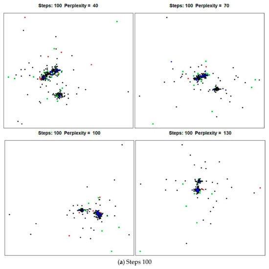
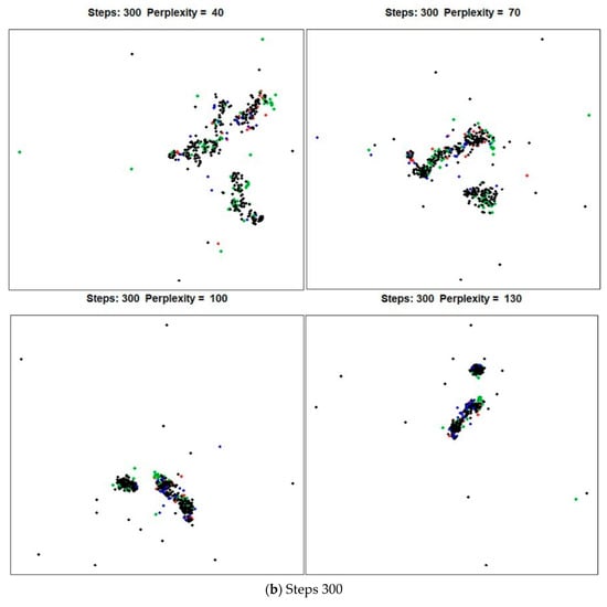
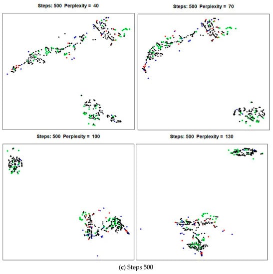
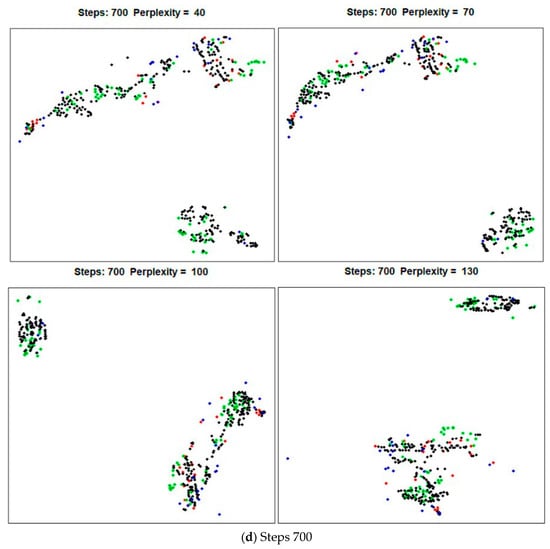
Figure 6.
t-SNE run results using different step numbers and perplexity limits for inventory classes: no landslide (red dots), landslide (black dots), vulnerable slopes (blue dots), and unlabeled (green dots). t-SNE, t-distributed stochastic neighbor embedding.
As a result, t-SNE naturally expands dense clusters and contracts sparse ones. It is not suited for finding outliers because the sample arrangement does not directly represent distance, as in PCA. However, the useful dimensionality reduction allows us to visualize data in 2D [26]. During t-SNE processing, parameter optimization changed the obtained results dramatically. While changes in the number of steps did not improve performance, increasing the value of perplexity yielded more preferred solutions.
Vulnerable slope locations, which may be considered as slow-moving landslides, had (in a certain extent) a close distribution pattern to landslides class locations. This is because they tend to share similar mother rock (mainly shale) from the Yeonil Formation of the Gyeongsang Basin formed in the third period of the Cenozoic Era. However, the vulnerable slopes class was clearly isolated from other classes (unlabeled and non-landslide).
Some overlapping between the feature classes was observed in some locations, as a result of (1) generalization in the delineation of points by the data provider, and (2) the additional random point (1359 locations) that was created during processing. No-landslide and landslide points occurred together because the no-landslide points are from the same period as the 1998 landslide events (i.e., they include slopes that were prone, but did not slide) and do not indicate absolute no-landslide regions (areas of very low slopes, for instance). We concluded that using other common grouping functions, like k-means or k-medoids, will not be able to group (classify) the inventory classes in a meaningful way, especially in small and complex study areas. t-SNE has significantly better visualization capacity through its expansion of dense clusters and contraction of sparse ones [27]. As a result, unlabeled locations were increasingly clustered around landslide locations, especially when using higher perplexity values.
4.2. Apriori Analysis Results
To run the association analysis, the antecedent data of the eight independent conditioning factors, each classified into five index values (Figure 7), and the consequent slope formation inventory data in four classes were stacked into one data frame. New counts of the inventory classes (after generating random values in the polygon around the original points) became landslide (2869), vulnerable slopes (151), unlabeled (730), and no-landslide (209). The selected conditioning factors had been previously shown to be effective in susceptibility analysis with landslide class alone [28].
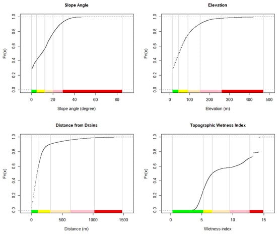
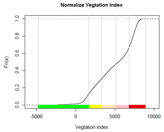
Figure 7.
Fisher’s Junks breaks in continuous conditioning factor values, green to red (very low, low, moderate, high, and very high).
Settings for the initial Apriori function parameters (support = 50%, confidence = 70%, max = 6%, and min = 2%) were applied to each class of the inventory separately. Generally, the conditioning factors included all five classes, but varied in amount. However, the distance to drains factors included just “low” and “very low” classes. Now, rather than mention each conditioning factor class and its corresponding frequency of inventory classes, the validity of using the association rules, offer to find the areas that share significant importance in landslide and unlabeled features occurrence with reference to other factor classes (Figure 8).
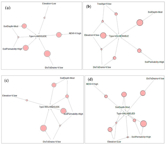
Figure 8.
Apriori analysis results showing the rules relating the antecedents to the consequents (in the center), lift value = 1 for all classes: (a) no-landslide (six rules and support 0.544–0.723). (b) Vulnerable (seven rules and support 0.522–0.713). (c) Landslide (six rules and support 0.521–0.744), and (d) unlabeled (eight rules and support 0.55–0.73).
Since there were many points in the landslide class compared to other classes, and to avoid the consequent risk of overfitting, we ran the function for each class separately. Apriori “association rules” were constructed in such a way that input could be adjusted according to its functionality. Conditioning factors, the “antecedent,” were placed on the left-hand side of the Apriori function, while the landslide inventory, the “consequent,” was placed on the right-hand side.
Figure 8 shows the relationship in terms of association rules for each inventory class. These were optimized by applying specific constraints for clear interpretation. The results, produced by the machine learning function, showed 50–76% support and 100% confidence using six, six, seven, and eight rules to describe the associations for the inventory classes, landslide, no-landslide, vulnerable slopes, and unlabeled, respectively.
The vulnerable slopes class represents slopes condition that did not cause slope failure over a long period, specifically from the main typhoons of 1998–2017. Consequently, according to field inspection, these areas were mostly on moderate slopes with thick vegetation cover and surrounded by different land uses such as infrastructure assets.
In this study, we sought to identify the original structure of the unlabeled class in the inventory; therefore, we identified the common antecedents that are particularly associated with that class.
Very low distance to drains (0–105 m) was found in all inventory classes, but was most common in landslide and unlabeled classes, reflecting observed landslide occurrence in most studies [29]. In a similar study, Althuwaynee et al. [28] produced landslide susceptibility maps that support this finding. In that work, in 40% of inventory locations identified as highly susceptible, drain distances were from 48 to 100 m. Very high NDVI values were evident in unlabeled and landslide areas, but not in vulnerable slopes and no-landslide areas, confirming that reliance on aerial photographs was not appropriate because of thick vegetation cover over the study area. In other studies, NDVI was not used (for this reason); however, forest age, density, and type were used [4]. Low elevation values (15–43 m msl) were associated with unlabeled and landslide classes, with less support for the latter. Elevation values were very low (0–15 m) in vulnerable slopes (with high support), but were insignificant in no-landslide class. The elevation layer was found to be insignificant in the identification of the occurrence of a landslide in another study [4] using chi-squared automatic interaction detection. High values of the soil permeability index (from high to somewhat excessive) were found with all classes in the inventory. However, in association with another antecedent (soil depth), it shows high support for most classes, except vulnerable slopes. Moderate soil depths (20–50 cm) occur over all the classes and are not considered an effective indicator to be used in association with the unlabeled data class. For soil thickness, which generally ranges from 0 to 100 cm, thicknesses between 50 and 100 cm have the highest susceptibility occurring in almost 88% of the training dataset. A thicker soil is likely to carry more water [30]. TWI was not significantly observed, by analysis, as antecedent factor to initiate or motivate the landslides.
Tree age, with very low intensity (short aged to non-forest), had little significance in the vulnerable slopes class but was insignificant in other classes, making this antecedent factor ineffective in the current study. This noneffectiveness accords with previous landslide susceptibility analysis [4,28].
4.3. Automatic Landslide Detection for Validation
To best identify landslides using change detection, we removed changed areas of one-pixel value (900 m2) and generated buffer circles of 300 m diameter around the original inventory locations. Figure 9 shows the results of change detection overlain on the original landslide inventory map. The results show that many active changes occurred around the unlabeled landslide data inventory (Figure 9).

Figure 9.
Results of 7/5 band ratio change detection.
Figure 10 summarizes the landslide location data obtained by automatic change detection for each landslide inventory polygon as follows.
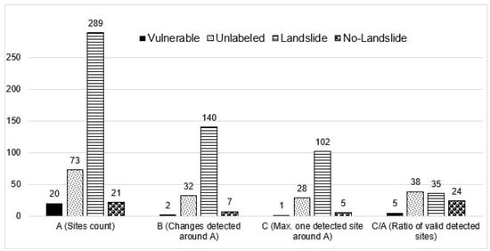
Figure 10.
Validation results using automatic change detection results.
- “A” represents the original inventory items count.
- “B” represents the total locations generated by the automatic classification change detection technique within all the inventory polygons (300 m diameter).
- “C” represents the maximum of one changes detected location per polygon in the study area.
- “C/A” represents is the ratio of polygons with a detected change to the number of original inventory items.
Figure 10 clearly shows that unlabeled and landslide have the largest numbers of locations (B). Any changes within a circle of 30 m diameter were considered as a single event, and that is shown as the value of C. Thus, C/A values are normalized detection values suggesting a valid relationship between landslide and unlabeled data locations, with the latter probably representing the missing (undocumented) landslides.
5. Conclusions
This research presents an economical solution, using machine learning with geospatial technology, to the classification of unlabeled slope structures using only the existing slope condition inventory (without need to carry out extensive fieldwork). The methodological process adopted here was designed sequentially to deliver insights into, or information about, the nature of unlabeled landslide inventory data. Thus, the results of each phase can be used as a standalone solution, or one can proceed with all phases for a higher degree of confidence (especially in cases where the inventory has a complex structure, or the study area is small with a semi-uniform surface).
Two machine learning algorithms were investigated with a multiclass inventory: first, nonlinear clustering t-SNE, which preserves as much of the significant structure of the high-dimensional data as possible in a low-dimensional map; and second, Apriori data mining to find the common rules of association between the inventory and the antecedent factors. These algorithms revealed, with acceptable degrees of confidence, the nature of the unlabeled data. However, without a validation step, significant doubt, arising from uncertainty in the data and the models, remains. Moreover, the rules of association for vulnerable slopes and no-landslide conditions were not effective in landslide or unlabeled slope identification, confirming a passive prediction capacity identified through a previous study in landslide susceptibility modeling in similar study area [4,28]. Therefore, an automatic change detection technique was used with actual optical images to verify the findings. Eventually, the objective was achieved with multiple validation tests and well-designed integrated methodology. Without needing extensive fieldworks, and using open data and an open coding environment, the presented approach will help with updating of any natural hazard’s incident inventory (medium or regional scale study area), as well as inventory that has different slope failures or slope conditions (creeps, unstable, etc.). Furthermore, this is especially useful in scarce data environments.
Author Contributions
Formal analysis, conceptualization, methodology, software: O.F.A.; data curation, conceptualization: I.-T.H. and Y.P.; writing—original draft preparation, review and editing: O.F.A., I.-T.H., A.A., Y.-K.L.; resource visualization, investigation: H.-J.P.; supervision, project administration, lab facilities, computers and hardware, research allowances: M.-S.L., S.-W.K. All authors have read and agreed to the published version of the manuscript.
Funding
This research was supported by Space Core Technology Development Program through the National Research Foundation of Korea funded by the Ministry of Science and ICT (2018M1A3A3A02066002), and MSIT (Ministry of Science, ICT), Korea, under the High-Potential Individuals Global Training Program (2019-0-01561) supervised by the IITP (Institute for Information & Communications Technology Planning and Evaluation). We express our gratitude to the Scientists Adoption Academy research network (scadacademy.com) to facilitate the research group meetings and results sharing.
Institutional Review Board Statement
Not applicable.
Informed Consent Statement
Not applicable.
Data Availability Statement
No new data were created or analyzed in this study. Data sharing is not applicable to this article.
Conflicts of Interest
The authors declare no conflict of interest and that they have no known competing financial interests or personal relationships that could have appeared to influence the work reported in this paper.
References
- Nilsen, T.H. Relative slope-stability mapping and land-use planning in the San Francisco Bay region, California. In Hillslope Processes; Routledge: London, UK, 2020. [Google Scholar]
- Althuwaynee, O.F.; Musakwa, W.; Gumbo, T.; Reis, S. Applicability of R statistics in analyzing landslides spatial patterns in Northern Turkey. In Proceedings of the 2017 2nd International Conference on Knowledge Engineering and Applications, ICKEA 2017, London, UK, 21–23 October 2017. [Google Scholar]
- Pokharel, B.; Althuwaynee, O.F.; Aydda, A.; Kim, S.-W.; Lim, S.; Park, H.-J. Spatial clustering and modelling for landslide susceptibility mapping in the north of the Kathmandu Valley, Nepal. Landslides 2020. [Google Scholar] [CrossRef]
- Althuwaynee, O.F.; Pradhan, B.; Park, H.J.; Lee, J.H. A novel ensemble decision tree-based CHi-squared Automatic Interaction Detection (CHAID) and multivariate logistic regression models in landslide susceptibility mapping. Landslides 2014, 11, 1063–1078. [Google Scholar] [CrossRef]
- Atangana Njock, P.G.; Shen, S.-L.; Zhou, A.; Lyu, H.-M. Evaluation of soil liquefaction using AI technology incorporating a coupled ENN/t-SNE model. Soil Dyn. Earthq. Eng. 2020, 130, 105988. [Google Scholar] [CrossRef]
- Brill, F.; Passuni Pineda, S.; Espichán Cuya, B.; Kreibich, H. A data-mining approach towards damage modelling for El Niño events in Peru. Geomat. Nat. Hazards Risk 2020, 11, 1966–1990. [Google Scholar] [CrossRef]
- Song, W.; Wang, L.; Liu, P.; Choo, K.K.R. Improved t-SNE based manifold dimensional reduction for remote sensing data processing. Multimed. Tools Appl. 2019, 78, 4311–4326. [Google Scholar] [CrossRef]
- Wong, K.Y.; Chung, F.-L. Visualizing Time Series Data with Temporal Matching Based t-SNE. In Proceedings of the International Joint Conference on Neural Networks, Budapest, Hungary, 14–19 July 2019; Department of Computing, Hong Kong Polytechnic University: Hong Kong, China, 2019. [Google Scholar]
- Halladin-Dabrowska, A.; Kania, A.; Kopeć, D. The t-SNE algorithm as a tool to improve the quality of reference data used in accurate mapping of heterogeneous non-forest vegetation. Remote Sens. 2020, 12, 39. [Google Scholar] [CrossRef]
- Agrawal, R.; Srikant, R. Fast Algorithms for Mining Association Rules. In Proceedings of the 20th International Conference on Very Large Data Bases, VLDB’94, Santiago de, Chile, Chile, 12–15 September 1994. [Google Scholar]
- Duaimi, M.G.; Salman, A. Association rules mining for incremental database. Int. J. Adv. Res. Comput. Sci. Technol. 2014, 2, 346–352. [Google Scholar]
- Guo, W.; Zuo, X.; Yu, J.; Zhou, B. Method for mid-long-term prediction of landslides movements based on optimized Apriori algorithm. Appl. Sci. 2019, 9, 3819. [Google Scholar] [CrossRef]
- Wu, X.; Zhan, F.B.; Zhang, K.; Deng, Q. Application of a two-step cluster analysis and the Apriori algorithm to classify the deformation states of two typical colluvial landslides in the Three Gorges, China. Environ. Earth Sci. 2016, 75, 1–16. [Google Scholar] [CrossRef]
- Aydda, A.; Algouti, A.; Algouti, A.; Essemani, M.; Taghya, Y. A new method to determine eroded areas in arid environment using Landsat satellite imagery. In Proceedings of the IOP Conference Series: Earth and Environmental Science, Jakarta, Indonesia, 23–24 January 2014. [Google Scholar]
- Kim, K.S. Methods for Investigation and Analysis of Landslides on Natural Terrain in Korea. Ph.D. Thesis, Andong National University, Andong, Korea, 2006. [Google Scholar]
- Park, J.H.; Park, S. Analysis of Instances of Characteristics Land Creep on the Mine Area in Korea. J. Korean Soc. For. Sci. 2018, 107, 393–401. [Google Scholar]
- Van Der Maaten, L.; Hinton, G. Visualizing data using t-SNE. J. Mach. Learn. Res. 2008, 9, 2579–2605. [Google Scholar]
- Wu, X.; Kumar, V.; Ross, Q.J.; Ghosh, J.; Yang, Q.; Motoda, H.; McLachlan, G.J.; Ng, A.; Liu, B.; Yu, P.S.; et al. Top 10 algorithms in data mining. Knowl. Inf. Syst. 2008, 14, 1–37. [Google Scholar] [CrossRef]
- Hahsler, M.; Grün, B.; Hornik, K. Arules—A computational environment for mining association rules and frequent item sets. J. Stat. Softw. 2005, 14, 1–25. [Google Scholar] [CrossRef]
- Toivonen, H. Apriori Algorithm. In Encyclopedia of Machine Learning and Data Mining; Springer: Berlin/Heidelberg, Germany, 2017. [Google Scholar]
- Althuwaynee, O.F.; Pradhan, B.; Lee, S. Application of an evidential belief function model in landslide susceptibility mapping. Comput. Geosci. 2012, 44, 120–135. [Google Scholar] [CrossRef]
- Jeong, G.-C.; Kim, K.-S.; Choo, C.-O.; Kim, J.-T.; Kim, M.-I. Characteristics of landslides induced by a debris flow at different geology with emphasis on clay mineralogy in South Korea. Nat. Hazards 2011, 59, 347–365. [Google Scholar] [CrossRef]
- van der Meer, F.D.; van der Werff, H.M.A.; van Ruitenbeek, F.J.A.; Hecker, C.A.; Bakker, W.H.; Noomen, M.F.; van der Meijde, M.; Carranza, E.J.M.; de Smeth, J.B.; Woldai, T. Multi- and hyperspectral geologic remote sensing: A review. Int. J. Appl. Earth Obs. Geoinf. 2012, 14, 112–128. [Google Scholar] [CrossRef]
- Aydda, A.; Althuwaynee, O.F.; Pokharel, B. An easy method for barchan dunes automatic extraction from multispectral satellite data. In IOP Conference Series: Earth and Environmental Science; IOP Publishing Ltd: Bristol, UK, 2020. [Google Scholar]
- Pezzotti, N.; Lelieveldt, B.P.F.; Van Der Maaten, L.; Höllt, T.; Eisemann, E.; Vilanova, A. Approximated and user steerable tSNE for progressive visual analytics. IEEE Trans. Vis. Comput. Graph. 2017, 23, 1739–1752. [Google Scholar] [CrossRef]
- Xu, W.; Jiang, X.; Hu, X.; Li, G. Visualization of genetic disease-phenotype similarities by multiple maps t-SNE with Laplacian regularization. BMC Med. Genomics 2014, 7, 1–9. [Google Scholar] [CrossRef]
- van der Maaten, L.; Hinton, G. User’s Guide for t-SNE Software. Structure 2008. Available online: https://sccn.ucsd.edu/svn/software/tags/EEGLAB7_0_2_9beta/external/fieldtrip-20090727/classification/toolboxes/maaten/tsne/tsne_user_guide2.pdf (accessed on 12 October 2020).
- Althuwaynee, O.F.; Pradhan, B.; Park, H.J.; Lee, J.H. A novel ensemble bivariate statistical evidential belief function with knowledge-based analytical hierarchy process and multivariate statistical logistic regression for landslide susceptibility mapping. Catena 2014, 114, 21–36. [Google Scholar] [CrossRef]
- Kayastha, P.; Dhital, M.R.; De Smedt, F. Application of the analytical hierarchy process (AHP) for landslide susceptibility mapping: A case study from the Tinau watershed, west Nepal. Comput. Geosci. 2013. [Google Scholar] [CrossRef]
- Lee, S.; Min, K. Statistical analysis of landslide susceptibility at Yongin, Korea. Environ. Geol. 2001. [Google Scholar] [CrossRef]


Publisher’s Note: MDPI stays neutral with regard to jurisdictional claims in published maps and institutional affiliations. |
© 2021 by the authors. Licensee MDPI, Basel, Switzerland. This article is an open access article distributed under the terms and conditions of the Creative Commons Attribution (CC BY) license (http://creativecommons.org/licenses/by/4.0/).