Abstract
In this study, a method is presented for estimating the number density of fine dust particles (the number of particles per unit area) through numerical simulations of multiply scattered ultrasonic wavefields. The theoretical background of the multiple scattering of ultrasonic waves under different regimes is introduced. A series of numerical simulations were performed to generate multiply scattered ultrasonic wavefield data. The generated datasets are subsequently processed using an ultrasound data processing approach to estimate the number density of fine dust particles in the air based on the independent scattering approximation theory. The data processing results demonstrate that the proposed approach can estimate the number density of fine dust particles with an average error of 43.4% in the frequency band 1–10 MHz (wavenumber × particle radius ≤ 1) at a particle volume fraction of 1%. Several other factors that affect the accuracy of the number density estimation are also presented.
1. Introduction
Airborne particulate matter, such as fine dust, is a global concern owing to its detrimental impact on human health [1,2,3,4]. Particles with a diameter of 10 μm or less (PM10) include dust from construction sites, industrial sources, and wind-blown dust from open lands. PM10 can cause eye, nose, and throat irritation and causes adverse health effects when it is inhaled into the lungs [5]. Particles with a diameter of 2.5 μm or less (PM2.5) can be emitted from the combustion of gasoline, diesel, and wood produce. The smaller particles (PM2.5) are more dangerous as they can enter the deep parts of the lungs and blood [5]. In this regard, the measurement of fine dust concentration has been recognized as a critical task for maintaining human health and there is an increasing need for accurate measurements of fine dust concentration.
Studies have been conducted to measure fine dust concentrations [6]. The available measurement techniques include the beta-attenuation method, gravimetric method, and light scattering method [7,8,9]. Among the various measurement methods, the light scattering method, which measures fine dust concentration by measuring scattered light intensity by airborne particles, is arguably the most widely accepted. This method allows for online measurements as well as low-cost, compact instrumentation. However, the light scattering method is an indirect method; the measured quantity is not an absolute physical quantity and requires additional calibration work to estimate the fine dust concentration. Moreover, it is susceptible to environmental factors, such as relative humidity, since light is an electromagnetic wave.
Unlike light, mechanical waves are less susceptible to changes in the electromagnetic properties of a medium (e.g., relative humidity), but they are sensitive to mechanical changes in a medium. Numerous studies have demonstrated the successful use of mechanical waves to characterize the mechanical properties of various media [10,11,12,13]. Mechanical waves have been employed to estimate particle concentration in various industrial applications [14,15]. Despite its potential, the authors were unable to find a work that reports the use of mechanical waves in measuring fine dust concentration.
In this study, we propose a mechanical wave-based method to estimate the number density of fine dust particles (the number of particles per unit area) in air. Here, the number density is defined as the number of particles per unit area rather than the number of particles per unit volume (in 3-D), because we performed 2-D simulation studies. The proposed method uses ultrasonic acoustic waves multiply scattered by fine dust particles in the air and the number density of fine dust particles is computed by processing the measured multiple scattering data based on the independent scattering approximation theory. The proposed number density estimation method was validated using ultrasonic wavefield data generated by a series of numerical simulations. The unique contributions of this study are: (1) the effective use of mechanical waves to estimate the number density of fine dust particles, (2) development of an ultrasonic wavefield data processing technique that directly computes the number density from measured wavefield data, and (3) understanding of the physical interaction between ultrasonic acoustic waves and fine dust particles randomly distributed in the air.
The remainder of this article is organized as follows: in Section 2 the theoretical background on the multiple scattering of acoustic waves in a discrete random medium is introduced; Section 3 describes the proposed ultrasound data processing approach to estimate the number density of fine dust particles; Section 4 provides details on the numerical simulations of multiply scattered ultrasonic wavefields; in Section 5 numerical simulation results of the number density estimation are demonstrated; in Section 6 we discuss several factors that affect the accuracy of the number density estimation.
2. Theoretical Background on Multiple Scattering of Acoustic Waves
Air with fine dust can be considered a discrete random medium where fine dust particles are randomly distributed within a background medium (i.e., air). When acoustic waves propagate through a discrete random medium, they interact with scatterers. The wave propagation lies in a different regime depending on the wave propagating distance (L) and scattering mean free path (lS), as illustrated in Figure 1. Here, lS is the characteristic length of the exponential decay of a coherent wave that propagates in its initial direction after taking ensemble averaging over multiple realizations of disorder [16].
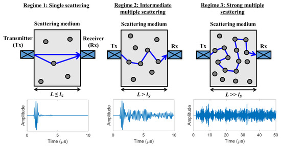
Figure 1.
Conceptual illustration of multiple scattering of acoustic waves. An example time-domain signal is displayed below the conceptual illustration of each regime. The scattering mean free path (lS) is the characteristic length of the exponential decay of a coherent wave that propagates in its initial direction after taking ensemble averaging over multiple realizations of disorder.
In the single-scattering regime (Regime 1), where L is comparable to or less than lS, unscattered and singly scattered wave components (presumably coherent waves) are dominant in the measured response. In this regime, the medium can be considered quasi-homogeneous, but with a renormalized wave speed. When the value of L is equivalent to a few mean free paths, single scattering becomes unimportant, and the wave propagation lies in the intermediate multiple scattering regime (Regime 2). In this regime, multiply scattered wave components are developed, but coherent waves are still observable with sufficient ensemble averaging. As L further increases to become much greater than lS, most wave energy is diffusively transferred by incoherent waves (Regime 3). In this regime, the transfer of the average wave intensity can be approximated by the diffusion equation. In this study, we focus on using coherent waves under Regimes 1 and 2 to estimate the number density of fine dust particles in the air, considering that acoustic wave propagation in the air–fine dust system typically lies in Regimes 1 and 2. Moreover, the independent scattering approximation (ISA) method, the basis of the proposed approach, works for Regimes 1 and 2 but not for Regime 3.
For a discrete random medium (e.g., air with fine dust), the solution of acoustic wave motion at the angular frequency ω and the position vector r given a point source location r’ can be represented as the summation of the incident wave and all possible waves scattered by the scatterers (e.g., random particles) [16]. It is given by:
where is the Green’s function (solution) of the homogeneous background medium (a non-scattering medium such as air without particles) at the frequency (ω) given the source position () and the receiver position (), and is the scattering potential at position (). represents the complete wave response solution including incident and all the scattered waves for the discrete random medium. Note that is a nonlocal operator that depends only on the distance between the source and receiver (), and it is expressed in the wavenumber (k) domain as:
where , and is the wave speed in the homogeneous background medium. Considering that Equation (1) is implicit, the exact closed-form solution for is not available. When the distance () is much shorter than lS, in Equation (1) can be approximated as , which is called the Born approximation. However, as the distance () increases, the Born approximate solution diverges from the actual solution. To obtain an accurate solution that considers the multiple scattering effects, the integral equation (Equation (1)) needs to be expanded to nearly infinite orders with respect to , which is computationally intractable.
Instead of seeking an exact solution for Equation (1), a statistical solution that is computationally tractable can be sought. Taking ensemble average responses, the mean Green’s function ⟨⟩ can be obtained as follows:
where the notation < > represents ensemble averaging and Σ is the self-energy that contains information about multiple scattering of acoustic waves. Equation (3) is known for the Dyson equation [17]. Note that the mean Green’s function <G> shown in Equation (3) is a nonlocal (translation-invariant) operator, similar to G0, unlike the Green’s function G shown in Equation (1). Then, the mean Green’s function in the k domain is given by
A comparison between Equations (2) and (4) reveals that the self-energy modifies the dispersion relation resulting in a modified wave speed and attenuation in the mean wavefield. Numerous multiple scattering theories have been proposed to model the self-energy term and hence to compute the effective wavenumber (ke) [18,19,20,21,22]. In this study, we incorporate the independent scattering approximation (ISA) method [22] to estimate the number density of fine dust in the air from the measured acoustic wave responses.
In the ISA method, each scatterer is assumed to be uncorrelated. The self-energy Σ is then expressed by the product of the scattering contribution of one scatterer and the number density (n) of scatterers
where is the T-matrix that describes the contribution of a single scatterer [23]. Within a certain range of frequencies where the wavelength is not much larger than the scatterers, the self-energy becomes independent of k. In this regime, the random medium can be considered a quasi-homogeneous medium (effective medium) with an effective wavenumber given by
Note that is a complex number whose real part is related to the phase velocity of the effective medium and imaginary part the attenuation. An important characteristic distance for coherent wave propagation is the mean free path lS given by
where α is the attenuation of the coherent wave. Within a few mean free paths, the coherent wave propagates with the speed of and decays exponentially with attenuation α. Here, the coherent wave attenuation is caused by scattering. In the ISA, lS is further related to the number density n, given by
where is the total scattering cross-section of one scatterer. Note that the theory introduced in this section can apply to both 2-D and 3-D conditions without loss of generality. In 2-D, n has a unit of (1/m2), and (m). In 3-D, n and have a unit of 1/m3 and m2, respectively. Equation (8) depicts the fundamentals of the proposed fine density estimation technique: the number density of scatterers can be estimated using α obtained from the ensemble average wave responses and the analytically computed . More detail about the ISA theory can be found in [22]. The proposed fine dust density estimation technique is detailed further in the following section.
3. Number Density Estimation Approach Based on Independent Scattering Approximation
An overview of the proposed fine dust number density estimation technique is presented in Figure 2. First, ensemble averaging is carried out over multiple realizations to obtain coherent wave responses ,
where M is the number of realizations, is the mth scanning measurement data, and is the ith sensor position at each realization. The coherent wave responses are subsequently converted from the time domain to the frequency domain using the Fourier transform below
where is the converted frequency-domain coherent wave response data. Here, the magnitude of the frequency-domain data can be represented as
where is the coherent wave magnitude at the first sensor position . The coherent wave attenuation is then computed by seeking the slope of the least-squares fit of , where
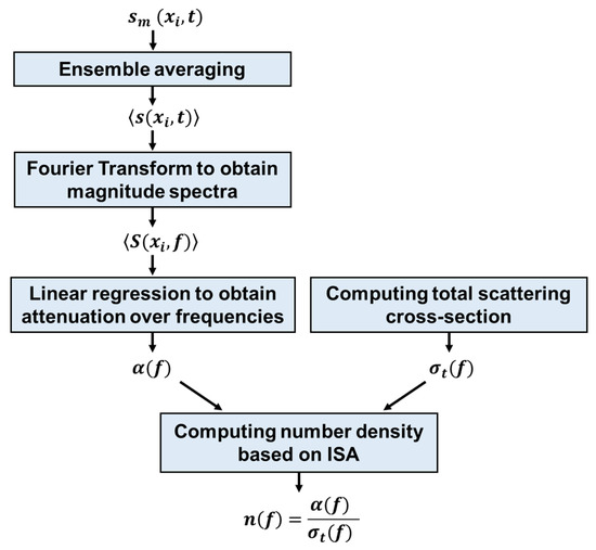
Figure 2.
Schematic of the proposed number density estimation approach.
Next, the total scattering cross-section for one fine dust particle is analytically computed. In this study, we use for the rigid cylindrical cavity seen in [24] to compute the number density of fine dust in the air, given by
where is the radius of the cylindrical cavity, and and are the Bessel function of the first kind and Henkel function of the second kind, respectively. Note that an additional elastic contribution term exists in when the scatterer is an elastic solid [25]. However, this term is negligibly small in the frequency range ( that is primarily used in this study; for example, ka is approximately 0.45 at the frequency of 5 MHz, which is employed in this study. Therefore, we use the rigid contribution of displayed in Equation (13) and neglect the elastic contribution when computing of a fine dust particle. Finally, the fine dust number density n is obtained based on the ISA described in the previous section, given by
Note that the obtained n can vary for each frequency, and it is represented by taking an average value of the n values across the excitation frequency band.
4. Numerical Simulations
Two-dimensional acoustic plane wave propagation in air with fine dust particles was simulated to generate acoustic wavefield data and evaluate the proposed number density estimation approach. A finite-difference time-domain (FDTD) simulation tool, k-wave, was used in this study [26]. The simulation was performed using a desktop computer with a graphical processing unit (GPU) (NVIDIA GeForce RTX 2060 Super), and the total calculation time per model was approximately 23 h.
The overall structure of the numerical simulation model is illustrated in Figure 3 and the numerical simulation parameters are summarized in Table 1. The simulated media represent 1425 μm × 57 μm air spaces where 10 μm fine dust particles were randomly spread out with different volume fractions (1, 2, 5, 10, and 15%). For each particle volume fraction case, two models with different particle placements were simulated. A spatially random distribution of dust particles is assumed to represent the air-particle system in reality. Perfectly matched layers (PMLs) [27] were added at the two ends of the simulation space to eliminate boundary reflections, as shown in Figure 3. PMLs were not added to the two edges parallel to the wave propagation path to model a plane wave incidence condition. Plane acoustic waves were generated with an excitation signal that was a linear chirp, across 0 to 10 MHz (see Figure 3), applied to the left end of the air space. We chose the frequency band (0–10 MHz) that gives a ka value below 1 to use the simplified analytical solution of the total scattering cross-section (Equation (13)). The corresponding acoustic wavefields were captured by a 35 × 30 sensor array at each model, as shown in Figure 3. Here, each of the 35 acoustic wave signals along the x-axis represented a signal set (1-D scan data) for a single realization . To obtain an ensemble-averaged signal set , multiple realizations were needed. For each volume fraction case with two medium models, 60 acoustic wave signal sets (30 signal sets per model) were obtained to give the number of ensemble averaging (M) of 60. Two separate models, each providing 35 signal sets, were simulated, instead of a unified model providing 60 signal sets, for each volume fraction case due to limited computation power.
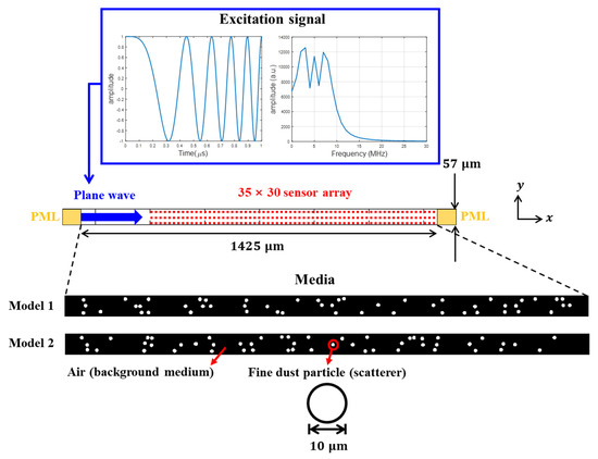
Figure 3.
The overall structure of the numerical simulation model. At each volume fraction case, two models that had different scatterer distributions were simulated to obtain acoustic wave responses across multiple realizations.

Table 1.
Summary of the numerical simulation parameters.
5. Results and Discussion
In this section, acoustic wavefield data generated by numerical simulations are presented, followed by the number density estimation results obtained by the proposed approach. Additionally, we discuss several factors that affect the number density estimation accuracy as well as the validity of ISA in number density estimation.
5.1. Multiply Scattered Acoustic Waves
Acoustic wavefields (represented by the particle velocity) for the 1% volume fraction case for a single realization and the ensemble-averaged wavefield with 60 realizations are shown in Figure 4a,b, respectively. Figure 4a represents and Figure 4b denotes . In these figures, wave rays with a positive slope indicate forward-propagating wave components and those with a negative slope indicate backward-propagating wave components. To clearly visualize incoherent wave components, the amplitude range (particle velocity) was limited to −1 to 1 m/s in Figure 4a,b. The single realization case (Figure 4a) displays a mixture of coherent forward-propagating waves and incoherent noise-like wave components that are set up by the network of fine dust particles. For the ensemble-average case (Figure 4b), the incoherent wave components that are distinct in Figure 4a are suppressed. Coherent forward-propagating waves are dominant in the ensemble-averaged wavefield and coherent back-scattering components are also observed. Acoustic wave signals at the first sensor position for the single realization and ensemble-average cases are depicted in Figure 4c,d, respectively. The two signals also demonstrate incoherent wave suppression by ensemble averaging.
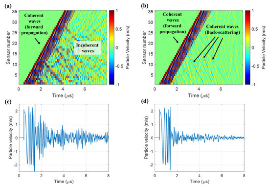
Figure 4.
Acoustic wavefields for the 1% volume fraction case: (a) wavefield for a single realization and (b) ensemble-average wavefield. Acoustic wave signals at the first sensor position for the two cases are shown in (c) and (d), respectively.
The coherent wave attenuation for the 1% volume fraction, computed using the coherent wavefield data presented in Figure 4b, is illustrated in Figure 5. As a reference, the ISA-based analytical attenuation computed by multiplying the analytical total scattering cross-section and the known number density value of 123 is also displayed. Overall, the coherent wave attenuation obtained using the simulation wavefield data exhibits good agreement with the analytical attenuation in the increasing trend over frequencies. However, as the frequency increases, the deviation between the two attenuation curves (data and analytical) becomes more distinct, revealing the possibility of number density estimation error.
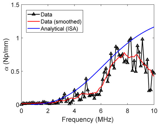
Figure 5.
Coherent wave attenuation for the 1% volume fraction case. An analytical attenuation curve computed using independent scattering approximation (ISA) is displayed as a reference. A smoothed coherent wave attenuation curve obtained by applying moving averaging is also displayed.
5.2. Number Density Estimation Results
The total scattering cross-section () used to compute the number density for a circular particle with a diameter of 10 μm is illustrated in Figure 6. The values were computed using the analytical solution in Equation (13) and a numerical simulation for a scattered wavefield by a circular particle. Here, the numerical simulation case models the scatterer as a circular particle having the material properties listed in Table 1, while the analytical solution assumes the scatterer to be a rigid cavity. Despite the discrepancy in the physical conditions of scatterers, the curves for the two cases are generally similar. In this study, we use the values computed by the analytical solution for number density computation, owing to its simplicity and ease of computation.
Figure 6.
Total scattering cross-section () for a circular particle in 2-D.
The number density values computed by the proposed approach are presented in Figure 7a. The exact number density value (123) is also indicated in the figure. Except for the low-frequency region (below 1 MHz), the estimated number density values are close to the exact number density with some variation. The mean and standard deviation of the estimated number density values in the frequency region between 1 MHz and 10 MHz are 99.18 and 91.83, respectively. The number density estimation error over the frequency region is displayed in Figure 7b. The estimation error varies with frequency. The mean of the estimation error within 1–10 MHz was 43.4%, and the minimum error was 1.19% at 1.88 MHz. Considering that the number density values were back-calculated from complicated wavefield data from a discrete random medium, the obtained number density values and the error level seem to be reasonable.
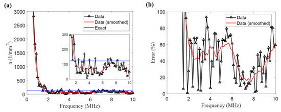
Figure 7.
Scatterer number density estimation results for the 1% volume fraction case: (a) computed number density and (b) estimation error. A zoom-in plot of the computed number density in the frequency region (1–10 MHz) is displayed in (a).
5.3. Effects of Particle Volume Fractions
To investigate the effects of particle volume fraction on the number density estimation accuracy, numerical simulation data for different particle volume fractions were used. Figure 8a–d present the number density estimation results (left) and estimation error (right) for volume fractions of 2%, 5%, 10%, and 15%, respectively. Along with Figure 7 (1% volume fraction), Figure 8 indicates that the estimated number density values over the frequency region of interest (1–10 MHz) become more deviant from the exact number density values as the volume fraction increases. In general, a higher estimation error is observed as the particle volume fraction increases. The higher errors observed in the cases with higher volume fractions are mainly because the scattering attenuation computed by the ISA is valid within lower volume fractions of scatterers [28].
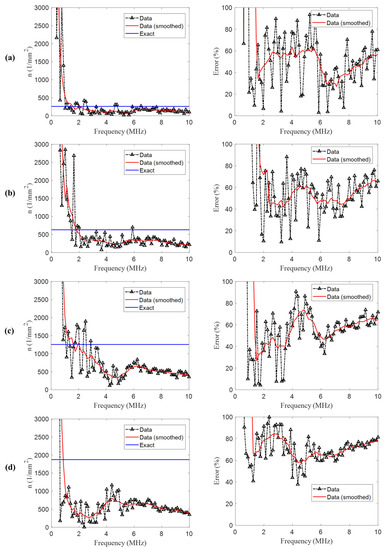
Figure 8.
Number density estimation results (left) and estimation error (right) for different scatterer volume fractions: (a) 2%, (b) 5%, (c) 10%, and (d) 15%.
Multiple scattering models can be divided into first-order and second-order models with respect to the number density [29]. The effective wavenumber (i.e., phase velocity and attenuation) computed by the first-order model is valid under lower number density media (roughly volume fractions below 10%). A second-order model, in most cases, provides higher accuracy when computing phase velocity and attenuation for higher number density media (higher volume fractions) [28], with a cost of higher computation complexity. Note that the ISA used in this study is inherently a first-order model. The ISA is selected as the basis of our approach, considering that it is computationally simple and most real-world applications may have a low volume fraction of fine dust particles, possibly below 1%.
In reality, the reported index of fine dust in the air is the mass concentration that can be obtained by multiplying the number density, mass density, and spherical volume of fine dust. The volume fractions (2–15%) considered in this study exceed the air quality guideline from the World Health Organization, which is 50 μg/m3 per day in the unit of mass concentration [30]. In other words, the volume fraction of fine dust, in reality, may be lower than 1%.
5.4. Effects of Particle Shapes
When computing a total scattering cross-section for a circular fine dust particle, the analytical solution for the case of a rigid circular cavity is used. This is because the scattering cross-section for a circular fine dust particle is similar to that for a rigid circular cavity (see Figure 6) and the rigid cavity case is computationally comprehensive. However, the shape of fine dust particles can vary in real-world applications.
The effects of varying particle shapes on the total scattering cross-section were investigated by considering six different particle shapes, as shown in Figure 9a. The upper three particle shapes (standard, ellipse, and two aggregated circles) were artificially designed by the authors, and the lower three particles (SEM 1 to 3) were obtained by image segmentation from scanning electron miscopy (SEM) images of actual fine dust particles. The total scattering cross-sections computed for the six particle shapes are depicted in Figure 9b along with those computed from the analytical solution (Equation (13)) with a cavity diameter of 2 μm. Figure 9b indicates that the scattering cross-section values vary significantly for the six particle shapes and are different from the analytical solution, especially at frequencies higher than 4 MHz. These results reveal that varying particle shapes can be sources of uncertainty when estimating the number density in real-world applications. Modeling the scattering cross-section as a point estimate can cause an erroneous number density estimation. Rather, we suggest the scattering cross-section as a probability distribution as an output across possible values. This approach can provide a probability distribution that enables not only the estimation of the number density but also the uncertainty quantification of the estimate.
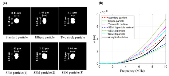
Figure 9.
Variations of scattering cross-section under varying scatterer shapes: (a) six different particle shapes and (b) their corresponding total scattering cross-sections.
6. Conclusions
This study investigates the application of ultrasonic multiple scattering features to estimate the number density (number of particles per unit area) of fine dust particles. We propose a number density estimation approach based on the independent scattering approximation theory. Based on the presented results, the following conclusions were drawn:
- Independent scattering approximation can be used to estimate the number density, especially when the volume fraction of fine dust particles is low.
- The proposed ultrasonic wave data processing approach enables the estimation of the number density of fine dust particles with an average error of 43.4% in the frequency band 1–10 MHz (ka ≤ 1) at a particle volume fraction of 1%.
- Variation of fine particle shapes is a cause of uncertainty in number density estimation.
Despite the potential to estimate the number density of fine dust particles in the air, the presented work has some limitations. The number density estimation performance varies across the studied frequency band, and the overall error in the number density estimation is still high (43.4%). In future work, we will further investigate how to improve the number density estimation performance and translate the proposed approach to an experimental system.
Author Contributions
Designed the study, H.S. and H.C.; performed numerical simulations, analyzed the simulation data, and drafted the manuscript, H.S. and U.W.; acquired the funding, supervised the study, reviewed, and improved the manuscript draft, H.C. All authors have read and agreed to the published version of the manuscript.
Funding
This study was supported by the Korea Agency for Infrastructure Technology Advancement (KAIA) grant funded by the Ministry of Land, Infrastructure and Transport (Grant 20CTAP-C151907-02).
Data Availability Statement
The data presented in this study are available on request from the corresponding author.
Conflicts of Interest
The authors declare no conflict of interest. The funders had no role in the design of the study; in the collection, analyses, or interpretation of data; in the writing of the manuscript; or in the decision to publish the results.
References
- Shridhar, V.; Khillare, P.S.; Agarwal, T.; Ray, S. Metallic species in ambient particulate matter at rural and urban location of Delhi. J. Hazard. Mater. 2010, 175, 600–607. [Google Scholar] [CrossRef]
- Jim, C.Y.; Chen, W.Y. Assessing the ecosystem service of air pollutant removal by urban trees in Guangzhou (China). J. Environ. Manag. 2008, 88, 665–676. [Google Scholar] [CrossRef]
- Nowak, D.J.; Crane, D.E.; Stevens, J.C. Air pollution removal by urban trees and shrubs in the United States. Urban For. Urban Green. 2006, 4, 115–123. [Google Scholar] [CrossRef]
- Pope, C.A.; Dockery, D.W. Health effects of fine particulate air pollution: Lines that connect. J. Air Waste Manag. Assoc. 2006, 56, 709–742. [Google Scholar] [CrossRef] [PubMed]
- Center for Disease Control and Prevention Particle Pollution. Available online: https://www.cdc.gov/air/particulate_matter.html (accessed on 10 December 2020).
- Amaral, S.S.; de Carvalho, J.A.; Costa, M.A.M.; Pinheiro, C. An overview of particulate matter measurement instruments. Atmosphere 2015, 6, 1327–1345. [Google Scholar] [CrossRef]
- Hauck, H.; Berner, A.; Gomiscek, B.; Stopper, S.; Puxbaum, H.; Kundi, M.; Preining, O. On the equivalence of gravimetric PM data with TEOM and beta-attenuation measurements. J. Aerosol Sci. 2004, 35, 1135–1149. [Google Scholar] [CrossRef]
- Giechaskiel, B.; Maricq, M.; Ntziachristos, L.; Dardiotis, C.; Wang, X.; Axmann, H.; Bergmann, A.; Schindler, W. Review of motor vehicle particulate emissions sampling and measurement: From smoke and filter mass to particle number. J. Aerosol Sci. 2014, 67, 48–86. [Google Scholar] [CrossRef]
- Chow, J.C.; Watson, J.G.; Park, K.; Lowenthal, D.H.; Robinson, N.F.; Park, K.; Maglian, K.A. Comparison of particle light scattering and fine particulate matter mass in central california). J. Air Waste Manag. Assoc. 2006, 56, 398–410. [Google Scholar] [CrossRef]
- Chimenti, D.E. Review of air-coupled ultrasonic materials characterization. Ultrasonics 2014, 54, 1804–1816. [Google Scholar] [CrossRef] [PubMed]
- Safaeinili, A. Air-coupled ultrasonic estimation of viscoelastic stiffnesses in plates. IEEE Trans. Ultrason. Ferroelectr. Freq. Control 1996, 43, 1171–1180. [Google Scholar] [CrossRef]
- Choi, H.; Song, H.; Tran, Q.N.V.; Roesler, J.R.; Popovics, J.S. Concrete International. 2016. Available online: https://www.concrete-international.nl/en/ (accessed on 20 December 2020).
- Zhang, J.; Drinkwater, B.W.; Wilcox, P.D. Defect characterization using an ultrasonic array to measure the scattering coefficient matrix. IEEE Trans. Ultrason. Ferroelectr. Freq. Control 2008, 55, 2254–2265. [Google Scholar] [CrossRef]
- Fu, S.; Lou, W.; Wang, H.; Li, C.; Chen, Z.; Zhang, Y. Evaluating the effects of aluminum dust concentration on explosions in a 20L spherical vessel using ultrasonic sensors. Powder Technol. 2020, 367, 809–819. [Google Scholar] [CrossRef]
- Kazys, R.; Sliteris, R.; Mazeika, L.; Van den Abeele, L.; Nielsen, P.; Snellings, R. Ultrasonic monitoring of variations in dust concentration in a powder classifier. Powder Technol. 2020, in press. [Google Scholar] [CrossRef]
- Tourin, A.; Derode, A.; Peyre, A.; Fink, M. Transport parameters for an ultrasonic pulsed wave propagating in a multiple scattering medium. J. Acoust. Soc. Am. 2000, 108, 503–512. [Google Scholar] [CrossRef]
- Sheng, P.; van Tiggelen, B. Introduction to wave scattering, localization and mesoscopic phenomena. Second edition. Waves Random Complex Media 2007, 17, 235–237. [Google Scholar] [CrossRef]
- Foldy, L.L. The multiple scattering of waves. I. General theory of isotropic scattering by randomly distributed scatterers. Phys. Rev. 1945, 67, 107–119. [Google Scholar] [CrossRef]
- Lax, M. Multiple scattering of waves. II. the effective field in dense systems. Phys. Rev. 1952, 85, 621–629. [Google Scholar] [CrossRef]
- Waterman, P.C.; Truell, R. Multiple scattering of waves. J. Math. Phys. 1961, 2, 512–537. [Google Scholar] [CrossRef]
- Lloyd, P.; Berry, M.V. Wave propagation through an assembly of spheres: IV. Relations between different multiple scattering theories. Proc. Phys. Soc. 1967, 91, 678–688. [Google Scholar] [CrossRef]
- Lagendijk, A.; Van Tiggelen, B.A. Resonant multiple scattering of light. Phys. Rep. 1996, 29, 143–215. [Google Scholar] [CrossRef]
- Tourin, A.; Fink, M.; Derode, A. Multiple scattering of sound. Waves Random Media 2000, 10, R31–R60. [Google Scholar] [CrossRef]
- Graff, K.F. Wave Motion in Elastic Solids; Dover Publications Inc.: New York, NY, USA, 1975; ISBN 0486667456. [Google Scholar]
- Derode, A.; Tourin, A.; Fink, M. Random multiple scattering of ultrasound. I. Coherent and ballistic waves. Phys. Rev. E Stat. Phys. Plasmas Fluids Relat. Interdiscip. Top. 2001, 64, 7. [Google Scholar] [CrossRef]
- Treeby, B.E.; Cox, B.T. k-Wave: MATLAB toolbox for the simulation and reconstruction of photoacoustic wave fields. J. Biomed. Opt. 2010, 15, 021314. [Google Scholar] [CrossRef] [PubMed]
- Berenger, J.P. A Perfectly Matched Layer for the Absorption of Electromagnetic Waves. J. Comput. Phys. 1994, 114, 185–200. [Google Scholar] [CrossRef]
- Chekroun, M.; Le Marrec, L.; Lombard, B.; Piraux, J. Time-domain numerical simulations of multiple scattering to extract elastic effective wavenumbers. Waves Random Complex Media 2012, 22, 398–422. [Google Scholar] [CrossRef]
- Kim, J.-Y. Models for wave propagation in two-dimensional random composites: A comparative study. J. Acoust. Soc. Am. 2010, 127, 2201–2209. [Google Scholar] [CrossRef]
- World Health Organization. WHO Air Quality Guidelines for Particulate Matter, Ozone, Nitrogen Dioxide and Sulfur Dioxide: Global Update 2005: Summary of Risk Assessment; World Health Organization: Geneva, Switzerland, 2006. [Google Scholar]


Publisher’s Note: MDPI stays neutral with regard to jurisdictional claims in published maps and institutional affiliations. |
© 2021 by the authors. Licensee MDPI, Basel, Switzerland. This article is an open access article distributed under the terms and conditions of the Creative Commons Attribution (CC BY) license (http://creativecommons.org/licenses/by/4.0/).