Applicability and Analysis of the Results of Non-Contact Methods in Determining the Vertical Displacements of Timber Beams

Abstract

Determining the displacements and consequent deformations of structures is a demanding branch of engineering. Displacements are most often determined by geodetic methods, among which high-precision non-contact methods have recently taken the lead. Engineering geodesy is an indispensable part of construction projects. In the desire for efficient and fast measurements, the technology of terrestrial laser scanning (TLS) and the use of robotic total station (RTS) and other geodetic methods are becoming more and more useful for engineers. In the presented study, we focused on the measurement and comparison of vertical displacements with various mentioned equipment and the determination of the influence of meteorological conditions on the displacements of timber beams that we used to perform the experiment. Measurements were performed both in the laboratory and outdoors. A novelty in the work was the use of a TLS scanner to determine the evaluation of small value displacements and the analysis of the usability of geodetic measuring equipment. In the Materials and Methods section, we describe the equipment used and the characteristics of the beams. The Results section describes the experimental outcomes, which include the performance of experimental analysis of vertical displacements of timber beams under different meteorological conditions. Altogether, the results consist of geodetic measurements and the processing of measured data. The results of measurements of vertical displacements with a terrestrial laser scanner were compared with the results obtained with a robotic total station were evaluated and compared with the displacements calculated from static analysis and the results of other methods used.

1. Introduction

Engineering geodesy is an essential part of construction projects, as it provides the necessary support in all phases of construction projects, from design to construction to recording of built facilities and infrastructure. The basic element of geodesy is the acquisition of spatial data of the earth’s surface and objects with the help of various geodetic measurement techniques and instruments. The applicability of non-contact methods for determining displacements and deformations is described in [1,2,3,4,5]. In addition, the analysis of various geodetic methods is carried out to determine displacements and their applicability and suitability for detecting displacements of smaller values. Among the described methods, the RTS method is in the forefront, which allows for automatic tracking of the target in motion and a sufficient number of measurements per second. Our work focused on the applicability of the terrestrial laser scanning (TLS) method, which has not been previously used for this type of research. We also compared the results with the applicability of the robotic total station (RTS) with other measurement tools and methods. The comparison of the experimental results with RTS show the high accuracy of the TLS measurements. When automatically tracking a measurement point, a parameter “number of measurements per second” is always defined, which can also be used to define dynamic parameters. Moreover, the tables show the results of other methods used. The experiment was performed on nine test specimens, three for each experiment, which corresponded to the [6] standards for testing timber beams. Calculations of deformations of timber beams were performed by SCIeng analysis, in order to compare the obtained results.

For many years, manual calculations were used to determine the statics of the structure, which required a good knowledge of the structure and the loads. When calculating the statics of a structure, we have to take into account all the additional parameters, such as moisture content of the material, density of the test specimen, weight and mass of the load, etc., which is a very demanding procedure when calculating the statics manually. Currently, at least in the field of engineering, the computer calculation of statics is a much simpler and reliable calculation procedure. In the procedure itself, with the help of programs, parameters can be entered, the load can be changed at will, and displacements can be simulated depending on the position of the load. The computer programs also allow us to better present the results in 3D or 4D technology.

Due to the constant development of computer technologies, the requirements for the representation of spatial data have changed. This allows users to improve the integrity of their spatial perception and, above all, to find spatial solutions at a higher level of quality. On the desire for efficient and fast measurements, the technology of TLS and RTS is becoming more and more useful for engineers.

The first 3D scanning technology was developed in the 1980s. The basic idea was to create as accurate a model as possible of the surface of various objects and buildings. The technology and use of 3D laser scanning took off in the 1990s when the scanners not only became more affordable but also became more accurate, faster, and able to realistically capture the environment [7]. The authors of [8] compared different methods for measuring the volume and deformations of a sand embankment. When using the TLS technology, they emphasized the high measurement accuracy and the simplicity and speed of field work. Focusing on the use of TLS to determine the deformation of structures, we note that a number of researchers have conducted similar studies Due to the mentioned advantages, the method may be suitable for monitoring deformations and displacements of structural elements. The authors of [9] determined the deformations and described the computational processing in the case of an arch beam loading. The applicability of the TLS scanner for monitoring infrastructure was investigated [10] in the case of a retaining wall [11], in the case of a bridge structure [12], in the case of a dam, and [13] in the case of a tunnel. A non-contact data acquisition technique is mainly used in areas where obtaining data by other methods is difficult.

Using TLS in combination with other deformation methods makes a lot of sense because the methods complement each other. Each measuring device has its own characteristics, so the use of several methods is highly recommended. In particular, the determination of small displacements or displacements within the reliability limits of the equipment is recommended, as described in [14]. The authors used a laser tracker in addition to the TLS and used both methods to determine the displacement of a small structure. Similar research can also be found in [15,16,17,18], where the authors describe the use and reliability of TLS to determine the deformation of structures.

Additionally, in the last decade, a lot of attention has been paid to determining displacements using RTS. This method gives us very accurate results, and the advantages are shown in the automatic sighting, registration, and tracking of measurement targets. Methods of data acquisition by RTS techniques to determine static and dynamic responses have been described in works [19,20,21,22,23,24,25,26,27,28,29,30,31,32].

Currently, TLS scanners are used for various purposes in the representation of the mutual relationships between objects and surroundings. They are also very suitable for BIM modelling of buildings and structures, for analysis of traffic accidents, and in architecture for reconstruction of buildings. In addition, they are used for various forms of monitoring, as described by the authors of [33,34,35,36,37,38,39,40,41,42,43,44,45,46,47,48,49,50,51,52,53,54,55,56,57,58,59,60,61,62,63,64,65,66,67,68,69]. In scan vs BIM methods for monitoring the progress of construction, the corresponding quality of the point cloud plays an important role, which has been studied in detail by the authors in [70].

The mentioned research confirmed the thesis that the use of TLS and RTS is suitable for performing measurements in hard-to-reach areas with an adequate number of stands and stabilization of support points for the point cloud georeferencing process.

The Purpose of the Research

The research had two goals—namely, to determine the vertical displacements of timber beams using non-contact methods under different conditions and to determine the behavior of timber beams under load. For this purpose, we used the TLS method, and for the comparison of results we also used the RTS technology, which is one of the most geodetically reliable methods. Geodetic instruments for leveling and total station of lower accuracy were also used. To perform the experiment, we used the available measuring equipment that we have at the Faculty of the University of Maribor. In our case, TLS technology was exposed in the laboratory to additional lighting and additional reflection of rays from reflex surfaces, and the technology was exposed in the open to increased humidity due to additional humidification of the beams. With additional humidification, we wanted to determine how the increased humidity affected the load-bearing capacity, and thus we also increased the air humidity. As is known from the available literature, only a change in humidity has an additional effect on the results obtained with both TLS and RTS technology. To avoid mistakes, we placed both instruments at an ideal distance of less than 10 m and perpendicular to the brackets, which allowed us the optimal angle. To analyze the results, we used the results obtained with a TLS Leica RTC 360 LT and RTS Leica TS 50. As a second goal, we set out to investigate the static load-bearing capacity of timber beams of the same type, which were exposed to different meteorological conditions but the same load. We chose timber beams because wooden construction represents a new trend in construction and timber beams often replace other building composites. For this purpose, the static load capacity of the beams was calculated, and the predicted vertical displacements were determined for the characteristic points on the beam. The bending tests were carried out according to the recommendations of EN 408 [6], which prescribe the performance of a 4-point bending test. The distance between the supports was 18 times the height (3960 mm), and the load points were located at one-third of the span.

All static loads and consequent stiffnesses are statically and strength-determined according to European regulation EN 408:2003. The regulation requires that the minimum effective length of the test piece (L*) should be 19 times the height of the test piece, thus ensuring a fully bending behavior of the member (tangential stresses are small). The test piece should be freely supported on two edge supports with a center-to-center spacing (L) 18 times the height of the test piece. The load is transmitted to the subject by two symmetrically located equal point forces whose distance (a) to the axis of the support can be chosen. A special steel backing plate can be inserted between the piston through which the force is transmitted and the test piece, the thickness of which must be less than half the thickness of the test piece, as shown in Figure 1.

The so-called “global” elastic modulus of the sample (E_m,g) can now be calculated analytically in the form (1):

$$E_{m,g} = \frac{L^3\cdot \left(F_2 - F_1\right)}{b{h}^3\cdot \left(w_2-w_1\right)}\cdot \left[\left(\frac{3a}{4L}\right) -{\left(\frac{a}{L}\right)}^3\right]$$

(1)

where w₂ − w₁ is the increment of the measured deflection by the increment of the loading force F₂ − F₁.

The same requirements as for the modulus of elasticity shall apply as those regarding the basic requirements of the tester. The static system as shown in Figure 1 above shall be used. The flexural strength of the test piece material (f_m) shall be calculated as (2):

$$f_m = \frac{a\cdot F_{\max }}{2W}$$

(2)

where W represents the resistance moment of the test piece. The characteristic value (f_m,k) is statistically determined by taking into account the 5% fractional fraction.

Six 4400 mm long beams C24 with dimensions 60 × 200 mm, which are used in the construction of houses, were used for the experiment. The beams were labeled TL (timber in laboratory), TO (timber outside) and TW (timber outside—wet) and the serial number of the beam. The TL beam series represented beams for measurements under laboratory room conditions, while the TO and TW beam series represented measurements under outdoor meteorological conditions under which the TW beam was additionally moist. In our paper, the results of vertical displacements are presented for three beams—one from each group. For further analysis and before the actual testing and loading of the timber beams, the current condition—timber moisture content, mass, volume, and characteristic density of the beams—was recorded. The meteorological data listed in

Table 1. Physical and material properties of timber C24.

Beam	Humidity (%)	m (kg)	V (m3)	ρk (kg/m3)	fm,k (MPa)
TL_01	10.	22.1	0.05808	380.51	24
TO_01	11.2	26.05	0.05808	448.52	24
TW_01	10.5	22.5	0.05808	388.12	24

Where: m is mass per unit area, V is volume, ρ_k is characteristic density, f_m,k is characteristic bending strength.

were needed for the static load calculation. The characteristic bending strength was determined by EN 338:2004 [71]. All three timber beams were certified as solid timber—spruce C24. The physical properties changed naturally during the measurements. That is, the difference in moisture content and mass between TW and TO, which is given in Table 1.

Representative measurement points were placed between beams spaced 66 cm apart. A total of 18 concrete blocks 29 × 39 × 19 cm were used to load the beam. The average weight of a single block was 25.8 kg, and the total applied load was 1.17 kN/m². Figure 2 and Figure 3 show the loads on the beam and the installed targets.

The experiment was carried out to verify the behavior of the timber beams under different meteorological conditions and the same load, as well as the applicability of the TLS method to determine the displacements. For this purpose, the beams were placed in the laboratory under constant weather conditions and outdoors where they were exposed to the weather. All loading events were recorded using available surveying equipment. Flat, black-and-white targets printed on white, plasticized A4 paper were positioned for georeferencing before performing the measurements. Five targets were placed inside and five targets outside the laboratory in highly visible locations.

2. Materials and Methods

To perform the experiment, we used the available measuring equipment that we had at the Faculty of the University of Maribor: Leica RTC 360 LT terrestrial laser scanner, 5 flat black and white laser scanning targets measuring 10 × 10 cm, 10 flat black and white laser scanning targets measuring 15 cm × 15 cm, robotic total station Leica Nova TS 50, total station Nikon DTM700, two electronic levelers (Zeiss and Leica), 4 self-adhesive reflection retro targets with dimensions 6 × 6 cm, geodetic Pentagon prism, 5 measuring tapes for levelling. Some of the equipment is shown in Figure 4, the technical data of the available equipment are given in

Table 2. The technical data of the available equipment.

	RTS	Sprinter	TLS	DTM 730	Zeiss Dini 10
Accuracy (angle)	0.5″ (0.15 mgon)		18″	1″to 3″
Accuracy (distance)	0.6 mm + 1 ppm	0.6 mm (per 1 km)	1 mm + 10 ppm	2 mm + 2 ppm	0.1 to 0.7 mm (per 1 km)
working range	1.5 m to 3500 m	2 to 100 m	0.5 m to 130 m	2 m to 2500 m	1.5 m to 100 m
Number of readings (per sec)	9	3	1 milion	3	5

.

To prepare for the measurements, the optimal stand positions of the instruments were determined before the measurements. Before and during the measurements, the relative humidity was measured:

• In the laboratory, the measurements were performed under the conditions of 1 October 2020. The air temperature was 21.2 °C, the relative humidity 51%.
• Outdoor measurements were performed on 5 October 2020 under meteorological conditions outside the laboratory. The air temperature was 16.5 °C, the relative humidity 70%.

The measured meteorological parameters were taken into account when balancing the data. Before starting the loads, TS 50 was used to determine the initial spatial coordinates in the local coordinate system for all points on the beams and in the surrounding area.

Determining the coordinates of all points is used for georeferencing point clouds and identifying identical points in different series of data capture. Coordinate points represent the zero state of the beams. Data registration with TS 50 was performed in 4 gyri, taking into account metrological conditions.

For the analysis of displacements, we used additional targets for TLS technology—namely, dimensions 10 × 10 cm and 15 × 15 cm. We decided to use the targets because we anticipated that geodetic reflex self-adhesive targets would cause registration problems due to beam reflection and light. Additional targets for TLS technology were used mainly for georeferencing and connection with the results of RTS technology. Reference targets and small-scale targets were placed in the space on the media for scanning. In addition, spatial coordinates were determined for these targets. Scanning was performed using medium resolution (6 mm at 10 m) automatic double scanning and HDR photography, which is most often used in practice, as it provides a wide range of implementation with a medium level of data-capture accuracy and time required for capture. It took 4 min 21 s to complete one scan.

Georeferencing is the transformation of a point cloud from the local coordinate system of a laser scanner into any reference coordinate system. Georeferencing can be performed based on reference points in the point cloud or based on the known position of the device. In our case, we used reference points for TLS and RTS technology.

The advantage of using targets is also reflected in the georeferencing process. Indirect georeferencing is performed on the basis of known coordinates of scanned targets in the reference coordinate system, which serve as reference points. We established a geodetic network of these using classical terrestrial methods. The reference points represented the starting point for the formation of transformation parameters between the local coordinate system of the scanner and the reference coordinate system. At least 3 support points are required for a successful transformation.

The computer processing process began with the registration of the scans. The complexity of the procedure depended on the number of captured scans from different positions and the coverage of these for quality registration. The number of stands was due to the size and geometry of the scanned object, as we could avoid blind spots and possible physical obstacles when working. Given that we were considering a single area or facility, it was necessary to connect the stands. The basic purpose of registration was to find the binding parameters that optimally converted the point cloud of the local scanner coordinate system into a single project coordinate system. This could be done through various registration methods, such as registration using binding points, using features, and iterative approximation [72].

Combined method of registration—i.e., cloud-to-cloud and using targets—is the most common way to register point clouds as it gives the best results. The basic principle was to use special targets when scanning, which we placed in the field of view of the scanner. Each target allowed optimal reflection of the laser beam. In this way, good target identification was enabled. The scanner detected the target and determined its center based on various algorithms. The center of each target thus represented an unambiguous and direct connecting point in two different scans. Based on identical points, the program automatically determined the transformation parameters of the spatial transformation between the local scanner coordinate system and enabled their merger into a single project coordinate system [73]. The use of three connection points was sufficient for determining the transformation parameters. Increasing the number of these increased the reliability and accuracy of matching the two point clouds. In addition to the number, the appropriate layout was also important. Targets should be arranged to allow adequate homogeneity of the point cloud in the core and at the outer edges of the scan [74].

The registration of the scans was done with the program Leica Cyclone Register 360, based on the cloud-to-cloud and target registration process. This process used modern registration algorithms and was an established and automated registration process for combining individual scans. After combining the point clouds, optimizing the registration, and completing the registration, a registration report was created for all cases in the mentioned software, which included a bundle report (registration of the point cloud before and after the load). In all cases, the total registration error was below 3 mm, with overlap above 84% and strength above 72%, which was base on the Calibration Certificate and ensured that the results were within the specification of the product.

For georeferencing, the combined point cloud was transformed into a selected coordinate system stabilized on laboratory and outdoor support points, as shown in Figure 5 and Figure 6.

After merging the scans and georeferencing, the relevant distances were measured using the “measure distance” function, comparing the point clouds (“cloud-to-cloud”) before loading and after the performed loading of the beams. The displacements were determined based on the change in the positions of the centric point of the target. Figure 7 shows an example of the determination of displacements in the middle of the TL_02 beam. The procedure was repeated for all targets on the beams.

3. Results

The goals of the experiment were to determine the applicability of geodetic non-contact methods for measuring displacements of timber beams and to check the static load-bearing capacity of beams under different meteorological conditions. To this end, we combined the two goals in a single, experiment. The focus was on the applicability of the TLS method for calculating displacements. To achieve the desired values, a comparative analysis and accurate calculation were performed for each medium.

First, the vertical displacements at a given load based on the performed measurements were determined for each beam. Second, the beam displacements were measured at the locations where the targets were placed (Figure 8). Third, the measurement results were compared with the calculated value of vertical displacements based on the static analysis of the beam.

To evaluate the results, the vertical displacements were determined using a Leica RTS NOVA TS 50 and Leica RTC 360LR. The difference was given by the measurement error |Δz|. The measurement error was different for each individual measurement, so the calculated error could not be generalized as a standard error. The measurement was affected by many factors, such as changes in humidity, variations in temperature, variations in pressure, and, last but not least, the skill of the operator; it was therefore necessary to calculate the error of measurement separately for each measurement, as can be seen in Table 2, where the accuracies of the instruments used are given. The obtained results are summarized in

Table 3. Differences and comparisons of measurements with static analyses of the beam TL_01.

TL_01
Target	Static Analyses	Leica RTC 360 LT			Leica RTS NOVA TS 50
	z [mm]	z [mm]	|Δz|[mm]	|Δz|[%]	z [mm]	|Δz|[mm]	|Δz|[%]
1	−4.9	−3.8	1.1	23.89	−5.0	0.1	0.14
2	−8.5	−6.9	1.6	19.48	−7.9	0.6	7.81
3	−9.8	−9.0	0.8	8.70	−9.8	0.0	0.00
4	−8.5	−7.1	1.4	17.14	−8.0	0.5	8.97
5	−4.9	−4.1	0.8	17.89	−5.1	0.2	2.14
TL_01
Target	Zeiss DiNi	Leica Sprinter			Nikon DTM 700
	z [mm/%]	z [mm]	|Δz|[mm]	|Δz|[%]	z [mm]	|Δz|[mm]	|Δz|[%]
1		−6.1	1.1	22.17	−4.7	0.2	5.86
2		−9.6	1.1	12.03	−8.2	0.3	4.31
3	−10.5 (6.51%)	−10.4	0.6	5.48	−10.4	0.6	5.49
4		−9.1	0.6	6.20	−9.1	0.6	6.20
5		−6.0	1.1	20.17	−6.0	1.1	20.17

,

Table 4. Differences and comparisons of measurements with static analyses of the beam TO_01.

TO_01
Target	Static Analyses	Leica RTC 360 LT			Leica RTS NOVA TS 50
	z [mm]	z [mm]	|Δz|[mm]	|Δz|[%]	z [mm]	|Δz|[mm]	|Δz|[%]
1	−4.1	−3.6	0.5	12.20	−3.9	0.2	4.88
2	−7.0	−5.9	1.1	16.19	−6.9	0.1	1.99
3	−8.1	−7.9	0.2	2.47	−8.1	0.0	0.00
4	−7.0	−5.8	1.2	17.61	−6.8	0.2	3.41
5	−4.1	−3.7	0.4	9.76	−4.0	0.1	2.44
TO_01
Target	Zeiss DiNi	Leica Sprinter			Nikon DTM 700
	z [mm/%]	z [mm]	|Δz|[mm]	|Δz|[%]	z [mm]	|Δz|[mm]	|Δz|[%]
1		−4.9	0.8	16.33	−5.0	0.9	18.00
2		−7.4	0.4	4.86	−7.5	0.5	6.13
3	−8.8 (8.64%)	−9.1	1.0	10.99	−9.3	1.2	12.90
4		−7.4	0.4	4.86	−7.7	0.7	8.57
5		−4.6	0.5	10.86	−4.9	0.8	16.33

and

Table 5. Differences and comparisons of measurements with static analyses of the beam TW_01.

TW_01
Target	Static Analyses	Leica RTC 360 LT			Leica RTS NOVA TS 50
	z [mm]	z [mm]	|Δz|[mm]	|Δz|[%]	z [mm]	|Δz|[mm]	|Δz|[%]
1	−4.6	−5.4	0.8	17.24	−4.8	0.2	4.21
2	−7.9	−8.9	1.0	12.52	−6.8	1.1	14.03
3	−9.1	−10.0	0.9	9.88	−9.8	0.7	7.68
4	−7.9	−9.0	1.1	13.78	−6.8	1.1	14.03
5	−4.6	−5.6	1.0	21.58	−4.7	0.1	2.04
TW_01
Target	Zeiss DiNi	Leica Sprinter			Nikon DTM 700
	z [mm/%]	z [mm]	|Δz|[mm]	|Δz|[%]	z [mm]	|Δz|[mm]	|Δz|[%]
1		−4.4	0.2	4.55	−4.8	0.2	4.04
2		−6.5	1.4	17.83	−7.5	0.4	5.47
3	−8.4 (7.69%)	−8.1	−1.0	10.99	−8.9	0.2	2.26
4		−6.8	−1.1	14.03	−7.3	0.6	8.36
5		−4.6	0.0	0.21	−4.5	0.1	2.38

. To illustrate the dispersion, the results are presented in the form of graphs in Figure 9, Figure 10, Figure 11, Figure 12, Figure 13 and Figure 14.

From the results of Figure 9, Figure 10 and Figure 11, we see that the results are comparable with the static calculation. In Figure 1, where we compared the displacements of the beam in the laboratory, we see that the curve obtained with a robotic total station and a classical total station fits best into the static calculation. The TLS method differs the most.

Figure 10 shows us the values of the carrier that were exposed to meteorological conditions. The RTS curve is closest to the static calculation, while the Nikon DTM and Leica Sprinter curves are the closest, which is attributed to the external variable conditions. Subject to the golden rule, no method deviates from the static calculation.

Figure 11 shows the results of the additionally moistened support and thus also the higher load. The Nikon DTM curve fits best into the static calculation, followed by the Leica Sprinter curve. In this case, the geodetic instruments were greatly affected by the increased humidity in the air, which has a great influence on the measurements. However, none of the results exceeded the limit of the golden rule.

As can be seen from the results presented in Figure 9, Figure 10 and Figure 11, different displacements were obtained despite the same load. Therefore, for beams TO_01 and TW_01, the causes can be found in the higher humidity and thus the increase in load. The load of one brick increased by 2.6 kg in the superstructure during the experiment. Given that the modulus of elasticity of the timber beam has a large influence on the displacements, more accurate results would be obtained by means of long-term tests—i.e., exposing the beams to this load for a longer period of time, e.g., 1, 3, 6, and 9 months—which may be the subject of our further investigations. A detailed analysis of the behavior of the beams is shown in the following subheadings.

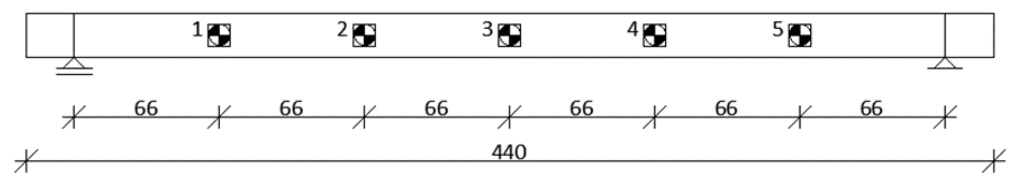
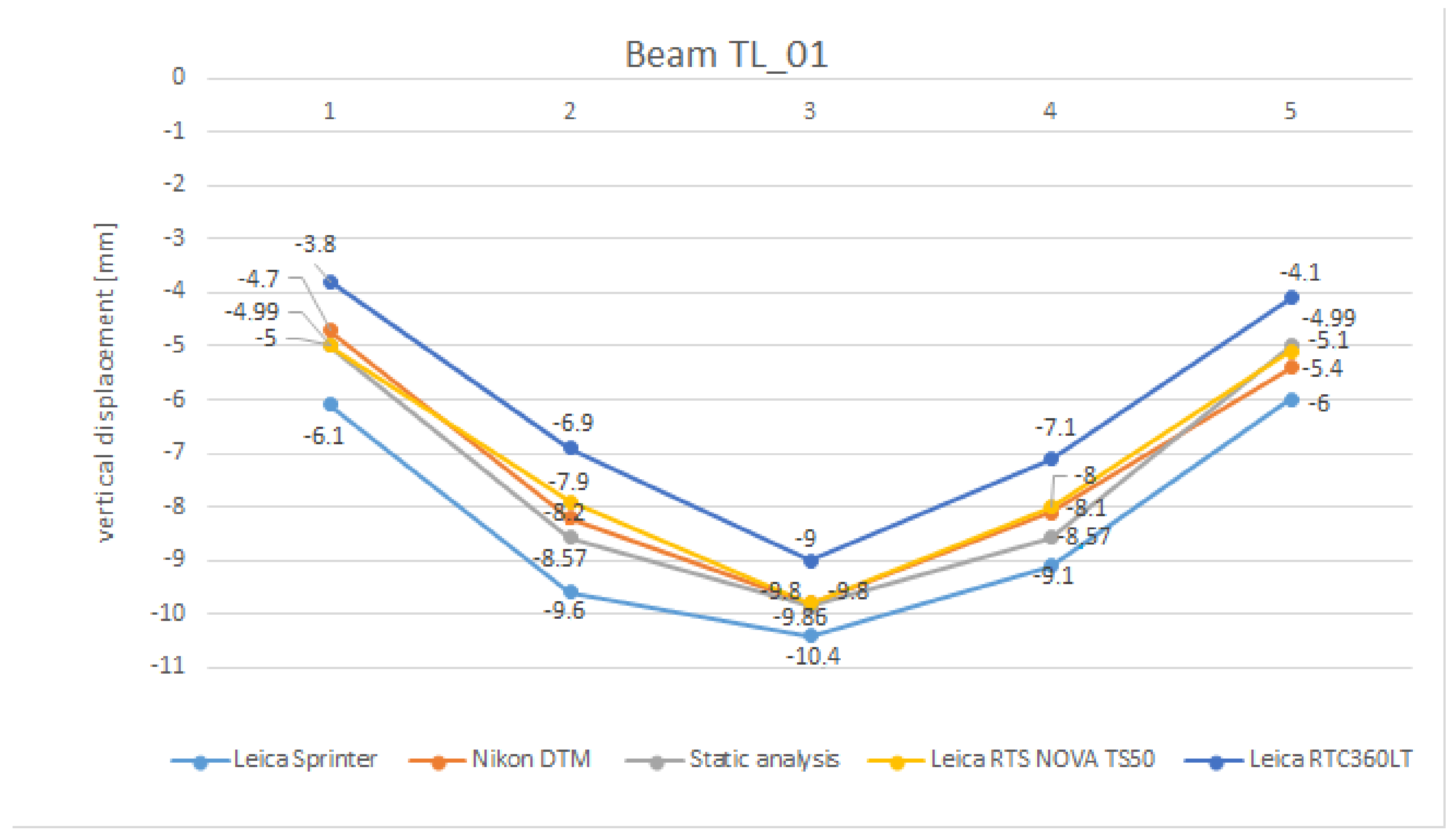
3.1. Timber Beam TL_01

The air temperature was 21.2 °C; the relative humidity was 51%. Temperature and pressure data are needed in the basic setup of measurements with geodetic instruments, which calculate meteorological corrections based on the input parameters. From the static analysis (Figure 12), it is possible to deduce the maximum vertical displacement that occurred in the middle of the beam (target 3), which was −9.858 mm. The vertical displacements measured by the RTC 360 LT were smaller compared with those calculated. The absolute value of the difference ranged from 0.858 mm (target 3) to 1.669 mm (target 2) and averaged 1.216 mm, which was comparable and had small deviations from the calculated values of vertical displacements (Figure 9 and Table 4). The error ranged from 0.007 mm (target 1) to 0.769 mm (target 4), with a mean of 0.322 mm. The calculated accuracy for the middle point of the beam was 0.822 mm (Table 3).

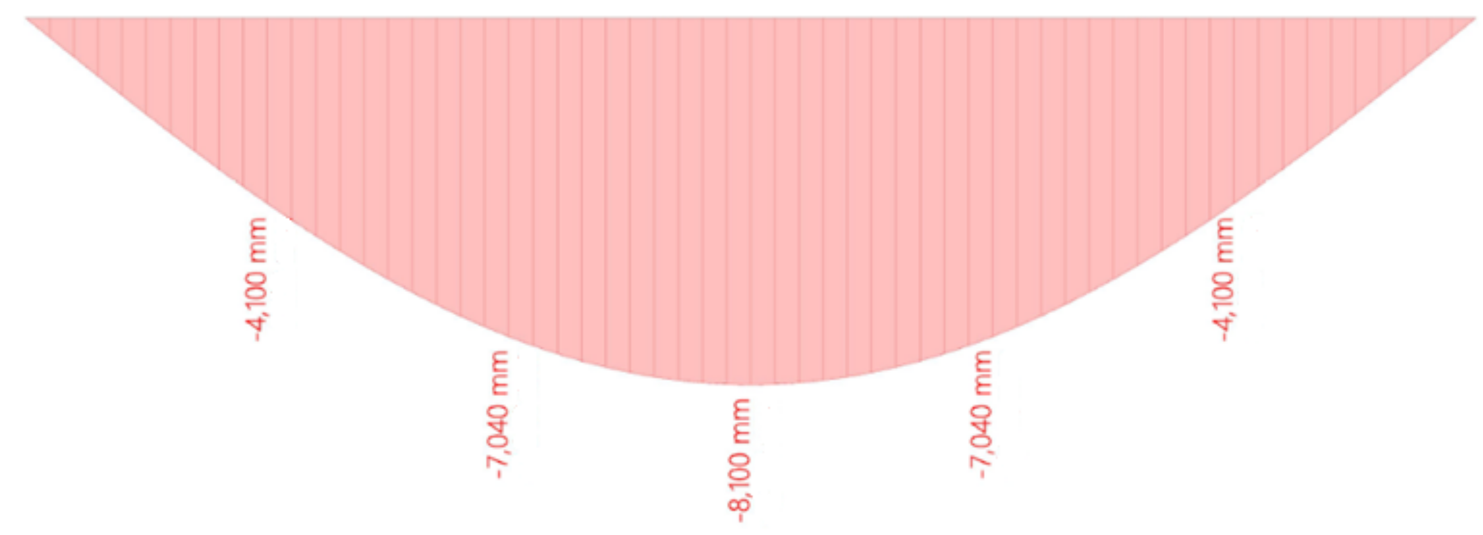
3.2. Timber Beam TO_01

The air temperature was 16.5 °C; the relative humidity was 70%. From the static analyses (Figure 13), the maximum vertical displacement could be calculated by introducing the so-called center of support (target 3) −8.1 mm. The vertical displacements measured by the RTC 360 LT were in the form of calculated minorities (Figure 10). The value of the error ranged from 0.200 mm (target 4) to 1.240 mm (target 4) and averaged 0.696 mm. The displacements obtained with RTS were more appropriate, which is also shown by the reduction in the curve in Figure 10. The average error value was 0.136 mm (Figure 10 and Table 4).

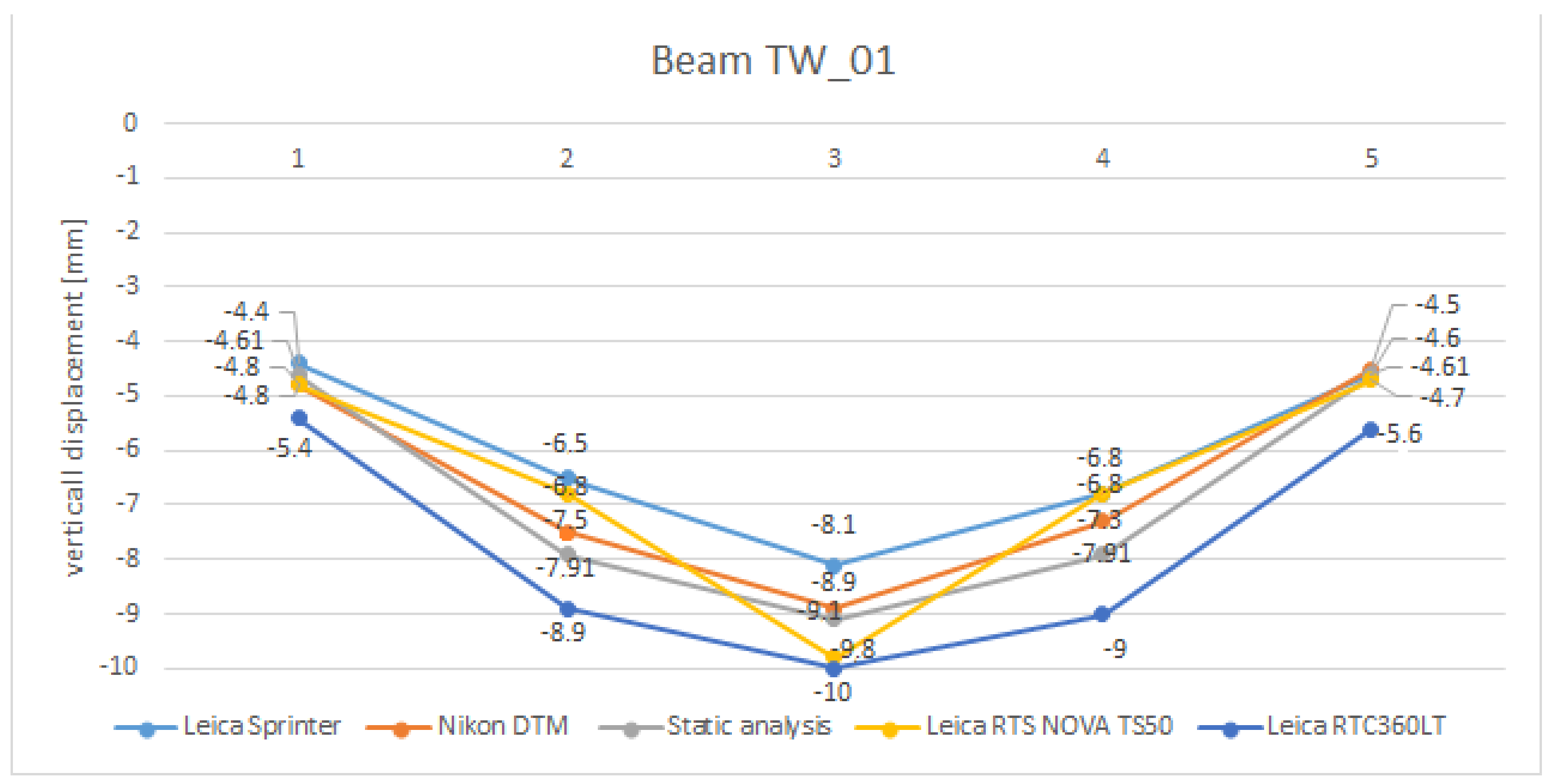
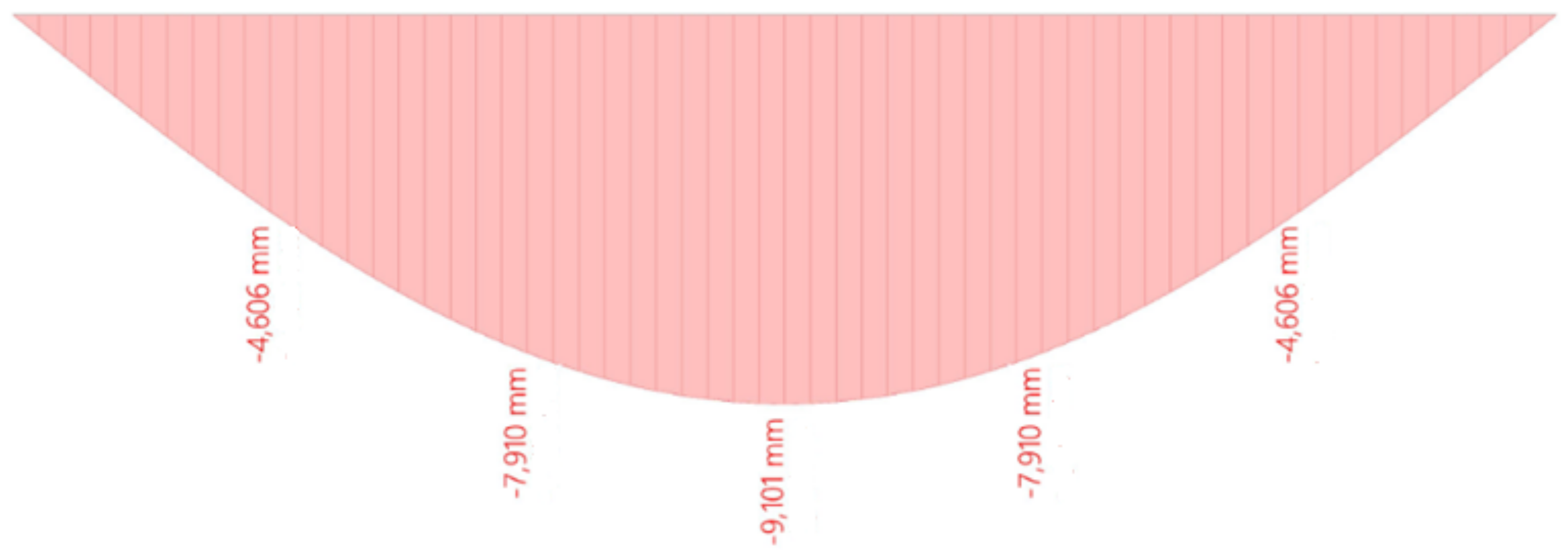
3.3. Timber Beam TW_01

The air temperature was 16.5 °C; the relative humidity was 70%. From the static analysis (Figure 14), the maximum calculated vertical displacement could be derived, which occurred in the middle of the beam (target 3) and was −9.1 mm. This time, the vertical displacements measured with the RTC 360 LT were higher than the calculated ones (Figure 11 and Table 5). The error values ranged from 0.794 mm (target 1) to 1.090 mm (target 5 and averaged 0.953 mm. The displacements determined with RTS were higher for targets 1, 3, and 5. The corresponding errors were: 0.194, 0.699, and 0.094 mm, respectively. In targets 2 and 4, the vertical displacements were smaller than calculated. The absolute value of the error was 1.110 mm. On average, the error was 0.247 mm (Table 5).

Figure 12, Figure 13 and Figure 14 show the results of the static analysis software SCIeng. These figures can be used to compare the experimental results with the numerically calculated values. A static model of a cantilever beam loaded with a permanent load along its entire length was considered.

4. Discussion

In the measurements, the results obtained with the TS 50 appear to be most consistent with the static calculation, which was to be expected since the TS 50 instrument is also the most accurate geodetic instrument. The TS 50 has an angular accuracy of 0.5″ (015 mgon) and a length accuracy of 0.6 mm +1 ppm, providing very accurate measurements. Given the length (7.05 m in the laboratory and 5.55 m outdoors) between the stand and the beam, the length error is negligible. In addition, the instrument was placed perpendicular to the midpoint which allowed clear reflection and minimal angular error. The smallest standard deviation of the measurements, which provides the precision of measurements from the calculated displacements of the static analysis, was at the center of the beam (target 3), where the largest vertical displacement for the single beam was also measured. For the measurements performed with RTC 360 LT, the absolute value of the difference between the calculated displacement and the measured displacement was less than 1 mm: 0.8 mm for beam TL_01 or 8.70% of the size of the calculated displacement, for beam TO _01 0.200 mm or 2.47%, and for beam TW_01 0.9 mm or 9.88%.

Calculations of deformations of timber beams were performed by SCIeng analysis, in order to compare the obtained results. If we compare only the highest obtained results—i.e., the results on the core of the carrier—we can see that the static analysis at TL_01 coincides with the results obtained with Nikon DTM 700 and RTS TS 50; at TO_01 it is comparable with RTS TS 50 and at TW_01 with Nikon DTM 700. We conclude that these two instruments could be the most authoritative. Further analyses have also confirmed this, but more detailed analyses would certainly require further investigations, which will also be carried out if the need arises.

Table 6. Comparison of measurement precision.

Beam	Leica RTC 360 LT		Leica RTS NOVA TS 50
	|Δz|[mm]	|Δz|[%]	|Δz|[mm]	|Δz|[%]
TL_01	1.2	17.42	0.3	3.93
TO_01	0.7	11.65	0.1	2.54
TW_01	0.9	15.00	0.2	8.40
Average	0.9	14.69	0.2	4.957

shows the comparison of measurement accuracy between the Leica RTC 360 LT and the Leica RTS NOVA TS 50, so as to consider the most accurate non-contact method. The results are presented for the midpoint of the beams.

Measurements made with the Leica RTC 360 LT terrestrial laser scanner, as a good laboratory alternative and contactless method, were found to be less accurate than those made with the Leica TS Nova TS 50. Furthermore, the difference between the calculated value and the measured value of the vertical displacement was on average 0.2 mm or 4.957% (Leica TS Nova TS 50), while this difference was 0.955 mm or 14.69% of the vertical displacement for the measurements with the RTC 360 LT.

Analysis of the measurement results of our experiment showed larger measurement errors for points that the scenario did not automatically detect. These points were entered manually into the program. The results thus show that the absolute value of the difference between the measured and calculated displacement value for these points was greater than 20%.

Table 6 shows that the lowest deviation from the displacements acquired from the static analysis was obtained for the measurements of TO_01 (11.65%). For the mentioned beam, the tripod was placed at a distance of 7.05 m, while for the other measurements the tripod was 5.55 m away from the beam. These distances are within a radius of 10 m, where the manufacturer guarantees maximum accuracy and minimum sampling scanning noise. For this purpose, additional research on the use of TLS for such measurements would be reasonable by changing the distance of the instrument within a radius of 10 m. It was found that the uneven influence of lighting conditions in laboratory on the accuracy of measurements made with the RTC 360 LT terrestrial laser scanner was significant. Measurements of TL_01 (1.2 mm and 17.42%) under artificial light conditions in the laboratory were less accurate than measurements outside the laboratory with TO_01 (0.7 mm and 11.65%) and TW_01 (0.9 mm and 15.00%). This can be mainly attributed to a larger number of reflecting surfaces in the laboratory, which affect the reflection of the laser beam and lead to imperfections in the point cloud of the scanned surroundings. The imperfections were visible in the form of the resulting holes in the point cloud, which could be eliminated by selecting a larger number of stands.

As one can see from the measurement results, there are some shifts in the reliability rank of the measurement devices. From the declarations of the used devices, we can conclude that displacements smaller than 1 mm cannot be considered as displacements because this is the maximum reasonable limit for geodetic measurements. If we wanted to measure displacements smaller than 1 mm, we would have to use other methods, such as inductive gauges, laser gauges, or precision dial gauges that offer a measurement accuracy of up to 0.01 mm.

Performing an experimental analysis of the displacements of timber beams aimed to evaluate the suitability of using terrestrial 3D laser scanning as a good laboratory alternative and non-contact method for determining the vertical displacements of structural elements. Based on the obtained results and existing literature, the findings can be summarized in the following points:

• Measurements made with the Leica RTC 360 LT terrestrial laser scanner were found to be less accurate than measurements made with the Leica Nova TS 50. The difference between the calculated value and the measured value of the vertical displacement was on average 0.2 mm for the measurements with the Leica Nova TS 50, while this difference was 0.9 mm for the measurements with the RTC 360 LT.
• A larger deviation of the vertical displacement measurements occurred with targets that were not automatically detected by the program and were therefore recorded manually.

5. Conclusions

Terrestrial laser scanning is a modern non-contact method of acquiring spatial data by measuring the distance between an instrument and an observed object using laser light. Measurements are made using terrestrial laser scanners with active sensors that operate in the visible and infrared spectrum of light.

The market for measuring instruments involves many manufacturers of high-quality measuring and computing equipment. On account of competition, the technology has become increasingly affordable for engineers in various technical disciplines. In addition to the price, which is often a determining factor in equipment purchases, other important elements of quality have been identified, such as scanner performance, accuracy and precision, scanning speed, laser dot resolution, range, field of view, target usability, camera features, and associated software. The advantages in the technology include the speed and relative ease of making measurements in the field, which played a significant role in conducting experiments. Working with the Leica RTC 360 LT terrestrial laser scanner involved more than just collecting measurement data during the scanning process. A necessary step in terms of the applicability of the technology is the computer processing. This process was divided into several work phases in the following order: registration of the scans, georeferencing of the point cloud, filtering of the point cloud, grid construction and modelling, and analysis and interpretation of the vertical beam displacements.

Based on the written results, and in line with the purpose of the article, terrestrial 3D laser scanning can be confirmed as a good laboratory alternative and non-contact method for determination of vertical displacements due to following advantages: (i) the method showed millimeter accuracy of the measurements performed, (ii) application in the field was fast and easy, and (iii) the results could be post-processed quickly using standard software and hardware.

References

1. Kovačič, B.; Motoh, T. Determination of static and dynamic response of structures with geodetic methods in loading tests. Acta Geod. Geophys. 2019, 54, 243–261. [Google Scholar] [CrossRef]
2. Kovačič, B.; Gubeljak, N.; Lubej, S. Experimental investigation of the effect of temperature on the structures in the measurement of displacements. Tech. Gaz. 2019, 26, 1010–1016. [Google Scholar]
3. Kovačič, B.; Kapović, Z. Precision and results reliability analysis of different instruments for investigating vertical micro-displacement of structures. Surv. Rev. 2005, 38, 190–203. [Google Scholar] [CrossRef]
4. Kovačič, B.; Muršec, L.; Lubej, S. Non-contact monitoring for assessing potential bridge damages, Topical Problems of Green Architecture. In Proceedings of the Civil and Environmental Engineering 2019 (TPACEE 2019), Moscow, Russia, 19–22 November 2019. [Google Scholar]
5. Kovačič, B.; Motoh, T.; Lubej, S. Experimental analysis of the dynamic responses of bridging objects with alternative non-contact method. In Proceedings of the E3S Web of Conferences, International Science Conference SPbWOSCE-2018 Business Technologies for Sustainable Urban Development, St. Petersburg, Russia, 10–12 December 2018. [Google Scholar]
6. European Committee for Standardization. EN 408:2010+A1:2012. Timber Structures—Structural Timber and Glued Laminated Timber—Determination of some Physical and Mechanical Properties. Available online: https://standards.iteh.ai/catalog/standards/cen/5adc63d2-e164-4b6e-9c2d-64dd8a9d6f19/en-408-2010 (accessed on 11 August 2010).
7. Ebrahim, M. 3D Laser Scanners: History, Applications, and Future; Faculty of Engineering, Assiut University: Assiut, Egypt, 2014. [Google Scholar]
8. Yakar, M.; Yilmaz, H.M.; Mutluoglu, O. Comparative Evaluation of Excavation Volume by TLS and Total Topographic Station Based Methods. Lasers Eng. 2010, 19, 331–345. [Google Scholar]
9. Yang, H.; Omidalizarandi, M.; Xu, X.; Neumann, I. Terrestrial Laser Scanning Technology for Deformation Monitoring and Surface Modelling of Arch Structures. Compos. Struct. 2016, 17, 173–179. [Google Scholar]
10. Vezočnik, R. Analiza Tehnologije Terestričnega Laserskega Skeniranja za Spremljanje Deformacij na Objektih. Ph.D. Thesis, University of Ljubljana, Ljubljana, Slovenija, 2011. [Google Scholar]
11. Truong-Hong, L.; Laefer, D.F. Application of terrestrial laser scanner in bridge inspection: Review and an opportunity. In Proceedings of the IABSE Symposium Report, Madrid, Spain, 3–5 September 2014; Volume 102. [Google Scholar]
12. González-Aguilera, D.; Gómez-Lahoz, J.; Sánchez, J. A New Approach for Structural Monitoring of Large Dams with a Three-Dimensional Laser Scanner. Sensors 2008, 8, 5866–5883. [Google Scholar] [CrossRef] [Green Version]
13. Li, J.; Wan, Y.; Gao, X. A new approach for subway tunnel deformation monitoring: High-resolution terrestrial laser scanning. ISPRS-Int. Arch. Photogramm. Remote Sens. Spat. Inf. Sci. 2012, 39, 223–228. [Google Scholar]
14. Xu, X.; Bureick, J.; Yang, H.; Neumann, I. TLS-based composite structure deformation analysis validated with laser tracker. Compos. Struct. 2018, 202, 60–65. [Google Scholar] [CrossRef]
15. Lovas, T.; Barsi, A.; Detrekoi, A.; Dunai, L.; Csak, Z.; Polgar, A.; Bereyi, A.; Kibedy, Z.; Szocs, K. Terrestrial Laserscanning in Deformation Measurements of Structures; International Archives of Photogrammetry, Remote Sensing and Spatial Information Sciences, Part 5 Commission V Symposium: Newcastle upon Tyne, UK, 2010; Volume XXXVIII. [Google Scholar]
16. Yang, H.; Xu, X.; Neumann, I. Deformation Behavior Analysis of Composite Structures under Monotonic Loads based on terrestrial laser scanning technology. Compos. Struct. 2018, 183, 594–599. [Google Scholar] [CrossRef]
17. Gordon, S.; Lichti, D.D. Modeling Terrestrial Laser Scanner Data for Precise Structural Deformation Measurement. J. Surv. Eng. 2007, 133, 2. [Google Scholar] [CrossRef]
18. Lienhard, W.; Ehrhart, M.; Grick, M. High frequent total station measurements for the monitoring of bridge vibrations. In Proceedings of the 3rd Joint International Symposium of Deformation Monitoring (JISDM), Vienna, Austria, 30 March–1 April 2016. [Google Scholar]
19. Leinhard, W.; Ehrhart, M. State of the art of geodetic bridge monitoring. In Proceedings of the International Workshop of Structural Health Monitoring (IWSHM), Stanford, CA, USA, 1–3 September 2015. [Google Scholar]
20. Celebi, M.; Sanli, A. GPS is Pioneering Dynamic Monitoring of Long-Period Structures. Earthq. Spectra 2002, 18, 47–61. [Google Scholar] [CrossRef]
21. Chen, Q.; Huang, D.F.; Ding, X.L.; Xu, Y.L.; Ko, J.L. Measurement of vibrations of tall buildings with GPS. In Proceedings of the Health Monitoring and Management of Civil Infrastructure Systems, Newport Beach, WA, USA, 4–8 March 2001; Volume 4337, pp. 477–483. [Google Scholar]
22. Roberts, G.W.; Meng, X.; Dodson, A.H. The use of kinematic GPS and triaxial accelerometers to monitor the deflections of large bridges. In Proceedings of the 10th FIG International Symposium on Deformation Measurement, Orange, CA, USA, 19–22 March 2001. [Google Scholar]
23. Ogaja, C.; Wang, J.; Rizos, C. Detection of Wind-induced Response by Wavelet Transformed GPS Solutions. J. Surv. Eng. 2003, 129, 99–104. [Google Scholar] [CrossRef]
24. Meng, X.; Dodson, A.H.; Roberts, G.W. Detecting Bridge Dynamic with GPS and Triaxial Accelerometers. Eng. Struct. 2007, 29, 3178–3184. [Google Scholar] [CrossRef]
25. Marendić, A.; Kapović, Z.; Paar, R. Possibilities of Surveying Instruments in Determination of Structures Dynamic Displacements. Geod. List. 2013, 3, 175–190. [Google Scholar]
26. Koo, K.Y.; Brownjohn, J.M.W. Structural health monitoring of the Tamar suspension bridge. Struct. Control. Health Monit. 2013, 20, 609–625. [Google Scholar] [CrossRef] [Green Version]
27. Psimoulious, S.; Stiros, S. Measuring deflections of a Short-span Railway Bridges Using Robotic Total Sation. J. Bridge Eng. 2013, 18, 182–185. [Google Scholar] [CrossRef]
28. Marendić, A.; Paar, R.; Grgac, I.; Damjanović, D. Monitoring of oscillations and frequency analysis of the railway bridge “sava” using robotic total station. In Proceedings of the 2nd Joint International Symposium on Deformation Monitoring (JISDM), Vienna, Austria, 6 March 2016. [Google Scholar]
29. Marendić, A.; Paar, R.; Duvnjak, I.; Buterin, A. Determination of dynamic displacements of the roof of spots hall arena zagreb, FIG. In Proceedings of the 6th International Conference on Engineering Surveying, Prague, Czech Republic, 3–4 April 2014. [Google Scholar]
30. Psimoulious, P.; Stiros, S. Measurement of Deflections and Oscillation Frequencies of Engineering Structures Using Robotic Theodolites (TS). Eng. Struct. 2007, 29, 3312–3324. [Google Scholar] [CrossRef]
31. Kopačik, A.; Kyronovič, P.; Kadlecikova, V. Laboratory tests of robotic stations. In Proceedings of the FIG Working Week, Cairo, Egypt, 16–21 April 2005. [Google Scholar]
32. Plekidis, V.; Tsakiri, M.; Makra, K.; Karakostas, C.; Klimis, N.; Sous, I. Evaluation of Dynamic Response and Local Soil Effects of the Evripos Cable-stayed Bridge Using Multi-Sensor Monitoring System. Eng. Geol. 2005, 179, 7–17. [Google Scholar]
33. Christian, T. Model-based Analysis and Evaluation of Point Sets from Optical 3D Laser Scanners. Ph.D. Thesis, Otto-von-Guericke University Magdeburg, Magdeburg, Germany, 2007. [Google Scholar]
34. Clark, J.; Robson, S. Accuracy of Measurements Made with A Cyrax 2500 Laser Scanner against Surfaces of Known Colors. In Proceedings of the XXth ISPRS Congress, Commission 4, Istanbul, Turkey, 12–23 July 2004. [Google Scholar]
35. Luebke, D.; Lutz, C.; Wang, R.; Woolley, C. Scanning Monticello; The Department of Computer Science, School of Engineering and Applied Science, University of Virginia: Charlottesville, VA, USA, 2002. [Google Scholar]
36. Comis, D. ARS Study Helps Farmers Make Best Use of Fertilizers, United States Department of Agriculture, Agricultural Research Service (ARS). Available online: https://www.ars.usda.gov/news-events/news/research-news/2010/ars-study-helps-farmers-make-best-use-of-fertilizers/ (accessed on 9 June 2010).
37. Blais, F.; Picard, M.; Godin, G. Accurate 3D acquisition of freely moving objects. In Proceedings of the 2nd International Symposium on 3D Data Processing, Visualization, and Transmission, 3DPVT, Thessaloniki, Greece, 6–9 September 2004; pp. 422–429. [Google Scholar]
38. Guidi, G.; Micoli, L.; Russo, M.; Frischer, B.; De Simone, M.; Spinetti, A.; Carosso, L. 3D digitization of a large model of imperial Rome. In Proceedings of the 5th International Conference on 3-D Digital Imaging and Modeling: 3DIM, Ottawa, ON, Canada, 13–15 June 2005. [Google Scholar]
39. Hansen, H.N.; Carneiro, K.; Haitjema, H.; De Chiffre, L. Dimensional Micro and Nano Metrology. CIRP Ann. 2006, 55, 721–743. [Google Scholar] [CrossRef]
40. Ingensand, H.; Ryf, A.; Schulz, T. Performances and experiences in terrestrial laser scanning. In Proceedings of the Optical 3-D Measurement Techniques VI, Athens, Greece, 22–27 May 2004. [Google Scholar]
41. Gruen, A.; Kahmen, H. (Eds.) Ground-Base Remote Sensing Observations and Systems for Monitoring Volcanic Clouds. In Proceedings of the International Volcanic Ash Task Force (IVATF), Second Meeting, International Civil Aviation Organization, Montreal, QC, Canada, 11–15 July 2011. [Google Scholar]
42. Kersten, T.; Sternberg, H.; Mechelke, K. Investigations into the accuracy behaviour of the terrestrial laser scanning system trimble GS100. In Proceedings of the Optical 3D Measurement Techniques VII, Vienna, Austria, 3–5 October 2005; pp. 122–131. [Google Scholar]
43. Mechelke, K.; Kersten, T.P.; Lindstaedt, M. Comparative investigations into the accuracy behaviour of the new generation of terrestrial laser scanning systems. In Proceedings of the Optical 3-DMeasurement Techniques VIII, Zurich, Switzerland, 9–12 July 2007; pp. 319–327. [Google Scholar]
44. Bauza, M.B.; Hocken, R.J.; Smith, S.T.; Woody, S.C. The development of a virtual probetip with application to high aspect ratio microscale features. Rev. Sci. Instrum. 2005, 76, 095112. [Google Scholar] [CrossRef]
45. Dorn, M. Landmark detection by a rotary laser scanner for autonomous robot navigation in sewer pipes. In Proceedings of the ICMIT, the second International Conference on Mechatronics and Information Technology, Jecheon, Korea, 4–6 December 2003; pp. 600–604. [Google Scholar]
46. Medina, A.; Gayá, F.; Pozo, F. Compact Laser Radar and Three-Dimensional Camera. J. Opt. Soc. Am. A 2006, 23, 800–805. [Google Scholar] [CrossRef] [PubMed]
47. Torben, M.; Hansen, M.; Hjorth, K. Lidar Wind Speed Measurements from a Rotating Spinner; Danish Research Database & Danish Technical University: Lyngby, Denmark, 2010. [Google Scholar]
48. Scopigno, R.; Bracci, S.; Franca, F.; Matteini, M. Exploring David. Diagnostic Tests and State of Conservation, 1st ed.; Giunti: Firenze, Italy, 2004; ISBN 88-09-03325-6. [Google Scholar]
49. Zhang, S.; Huang, P. High-resolution, real-time 3-D shape measurement. Opt. Eng. 2006, 45, 123601. [Google Scholar]
50. Larsson, S.; Kjellander, J.A.P. Motion control and data capturing for laser scanning with an industrial robot. Robot. Auton. Syst. 2006, 54, 453–460. [Google Scholar] [CrossRef]
51. Na, K.-M.; Lee, K.; Shin, S.-K.; Kim, H. Detecting Deformation on Pantograph Contact Strip of Railway Vehicle on Image Processing and Deep Learning. Appl. Sci. 2020, 10, 8509. [Google Scholar] [CrossRef]
52. Yrttimaa, T.; Luoma, V.; Saarinen, N.; Kankare, V.; Junttila, S.; Holopainen, M.; Hyyppä, J.; Vastaranta, M. Structural Changes in Boreal Forests Can Be Quantified Using Terrestrial Laser Scanning. Remote Sens. 2020, 12, 2672. [Google Scholar] [CrossRef]
53. Szostak, M. Automated Land Cover Change Detection and Forest Succession Monitoring Using LiDAR Point Clouds and GIS Analyses. Geosciences 2020, 10, 321. [Google Scholar] [CrossRef]
54. Chan, T.O.; Xia, L.; Lichti, D.D.; Sun, Y.; Wang, J.; Jiang, T.; Li, Q. Geometric Modelling for 3D Point Clouds of Elbow Joints in Piping Systems. Sensors 2020, 20, 4594. [Google Scholar] [CrossRef]
55. Cigna, F.; Tapete, D.; Lu, Z. Remote Sensing of Volcanic Processes and Risk. Remote Sens. 2020, 12, 2567. [Google Scholar] [CrossRef]
56. Yin, C.; Li, H.; Hu, Z.; Li, Y. Application of the Terrestrial Laser Scanning in Slope Deformation Monitoring: Taking a Highway Slope as an Example. Appl. Sci. 2020, 10, 2808. [Google Scholar] [CrossRef] [Green Version]
57. Bakuła, K.; Pilarska, M.; Salach, A.; Kurczyński, Z. Detection of Levee Damage Based on UAS Data—Optical Imagery and LiDAR Point Clouds. ISPRS Int. J. Geo-Inf. 2020, 9, 248. [Google Scholar] [CrossRef] [Green Version]
58. Tralli, D.M.; Blom, R.G.; Zlotnicki, V.; Donnellan, A.; Evans, D.L. Satellite remote sensing of an earthquake, volcano, flood, landslide and coastal inundation hazards. ISPRS J. Photogram. Remote Sens. 2005, 59, 185–198. [Google Scholar] [CrossRef]
59. Kussul, N.; Skakun, S.; Shelestov, A.; Lavreniuk, M.; Yailymov, B.; Kussul, O. Regional-scale crop mapping using multi-temporal satellite imagery. Int. Arch. Photogram. Remote Sens. Spat. Inf. Sci. 2015, 40, 45–52. [Google Scholar] [CrossRef] [Green Version]
60. Weintrit, B.; Osińska-Skotak, K.; Pilarska, M. Feasibility study of flood risk monitoring based on optical satellite data. Misc. Geogr. 2018, 22, 172–180. [Google Scholar] [CrossRef] [Green Version]
61. Yen, B.C. Hydraulics and Effectiveness of Levees for Flood Control. In the US–Italy Research Workshop on the Hydrometeorology, Impacts, and Management of Extreme Floods. 1995. Available online: https://www.engr.colostate.edu/ce/facultystaff/salas/us-italy/papers/44yen.pdf (accessed on 14 April 2020).
62. Long, G.; Mawdesley, M.J.; Smith, M.; Taha, A. Simulation of airborne LiDAR for the assessment of its role in infrastructure asset monitoring. In Proceedings of the 13th International Conference on Computing in Civil and Building Engineering, Nottingham, UK, 30 June–2 July 2010. [Google Scholar]
63. Kurczyński, Z.; Bakuła, K. SAFEDAM-zaawansowane technologie wspomagające przeciwdziałanie zagrożeniom związanym z powodziami. Arch. Fotogram. Kartogr. Teledetekcji 2016, 28, 39–52. [Google Scholar]
64. Tournadre, V.; Pierrot-Deseilligny, M.; Faure, P.H. UAV photogrammetry to monitor dykes-calibration and comparison to terrestrial lidar. Int. Arch. Photogram. Remote Sens. Spat. Inf. Sci. 2014, 40, 143. [Google Scholar] [CrossRef] [Green Version]
65. Zhou, Y.; Rupnik, E.; Faure, P.H.; Pierrot-Deseilligny, M. GNSS-assisted integrated sensor orientation with sensor pre-calibration for accurate corridor mapping. Sensors 2018, 18, 2783. [Google Scholar] [CrossRef] [Green Version]
66. Bakuła, K.; Ostrowski, W.; Szender, M.; Plutecki, W.; Salach, A.; Górski, K. Possibilities for using lidar and photogrammetric data obtained with an unmanned aerial vehicle for levee monitoring. Int. Arch. Photogram. Remote Sens. Spat. Inf. Sci. 2016, 41, 773–780. [Google Scholar] [CrossRef] [Green Version]
67. Baltsavias, E.P. A comparison between photogrammetry and laser scanning. ISPRS J. Photogram. Remote Sens. 1999, 54, 83–94. [Google Scholar] [CrossRef]
68. Kim, H.; Pyo, H.; Kim, H.; Kang, H.W. Multi-Lens Arrays (MLA)-Assisted Photothermal Effects for Enhanced Fractional Cancer Treatment: Computational and Experimental Validations. Cancers 2021, 13, 1146. [Google Scholar]
69. Cariou, E.; Baltzer, A.; Leparoux, D.; Lacombe, V. Collaborative 3D Monitoring for Coastal Survey: Conclusive Tests and First Feedbacks Using the SELPhCoAST Workflow. Geosciences 2021, 11, 114. [Google Scholar] [CrossRef]
70. Rebolj, D.; Pučko, Z.; Čuš Babič, N.; Bizjak, Z.; Mongus, D. Point cloud quality requirements for Scan-vs-BIM based automated construction progress monitoring. Autom. Constr. 2017, 84, 323–334. [Google Scholar] [CrossRef]
71. EN 338:2004. Structural Timber—Strength Classes; European Committee for Standardization: Brussels, Belgium, 2009. [Google Scholar]
72. Smogavec, L. Uporabnost Terestričnega Laserskega Skeniranja Pri Izdelavi Geodetskega Načrta. Ph.D. Thesis, University of Ljubljana, Ljubljana, Slovenija, 2015. [Google Scholar]
73. Opravš, P. Postopek in Natančnosti Tehnologije 3R Terestričnega Laserskega Skeniranja. Ph.D. Thesis, University of Ljubljana, Ljubljana, Slovenija, 2008. [Google Scholar]
74. Đapo, A. Terestričko Lasersko Skeniranje; Faculty of Geodesy, University of Zagreb: Zagreb, Croatia, 2008. [Google Scholar]
Figure 1. Example of load determination.
Applsci 11 08936 g001
Figure 2. Setting up and loading a timber beam in the laboratory (TL).
Applsci 11 08936 g002
Figure 3. Setting up and loading of the two timber beams outside (TO and TW).
Applsci 11 08936 g003
Figure 4. Measuring equipment used and marked measuring points (Leica TS 50, Nikon DTM700, Zeiss DiNi10, Leica Sprinter 100, Leica RTC 360 LT, retro target).
Applsci 11 08936 g004
Figure 5. Georeferencing and input of support points when measuring the beam TL_01.
Applsci 11 08936 g005
Figure 6. Identification of support points of the combined point cloud required for transformation into the selected coordinate system.
Applsci 11 08936 g006
Figure 7. Evaluation of TL_02 beam displacements based on changes in target positions before and after loading.
Applsci 11 08936 g007
Figure 8. Sketch of target positions with corresponding markings.
Applsci 11 08936 g008
Figure 9. Comparison of the results of the vertical displacements of the beam TL_01.
Applsci 11 08936 g009
Figure 10. Comparison of the results of the vertical displacements of the beam TO_01.
Applsci 11 08936 g010
Figure 11. Comparison of the results of vertical displacements of the beam TW_01.
Applsci 11 08936 g011
Figure 12. Results of the static analysis of vertical displacements of the beam TL_01.
Applsci 11 08936 g012
Figure 13. Results of the static analysis of vertical displacements of the beam TO_01.
Applsci 11 08936 g013
Figure 14. Results of static analysis of vertical displacements of the beam TW_01.
Applsci 11 08936 g014