Instantaneous Frequency Representation Used for CPA Laser Simulation

Abstract

In the current study, we present a novel intuitive graphical method for the simulation of nonlinear effects on stretched pulses, characterized by a large time-bandwidth product. By way of example, this method allows precise determination of effects occurring in CPA (chirped pulse amplification) laser chains, such as the pre-pulse generation by the nonlinear Kerr effect. This method is not limited to first-order dispersion and can handle all resulting distortions of the generated pre-pulse.

1. Introduction

Ultra-intense laser systems are used for a variety of applications in the fields of high-energy-density physics and relativistic laser plasma physics [1]. Achievable contrast ratios are in the range of 10⁻¹² on temporal scales between ns and a few 10 ps prior to the main pulse. Amplification of stretched pulses (i.e., chirped pulse amplification, CPA [2]) is conventionally performed in regenerative and multipass amplifiers. Despite its capacity to lower nonlinearities in the amplifiers, the CPA technique, when used for an extremely high-power system (PW range), still accumulates nonlinear distortions due to the Kerr effect, which is characterized by the maximum value of the B-integral. The B-integral represents the nonlinear temporal phase shift acquired after propagation through the system. Typical levels of the B-integral are in the range of 0.1 to 1 [3,4,5,6]. To simulate the consequence of this nonlinearity on the temporal profile of the output beam, the simulation of nonlinear effects on stretched pulses with large time-bandwidth products is required. As an example, recent observations [6] have shown that the temporal characteristics of a pre-pulse may differ significantly from the main and post pulses from which it was generated via temporal diffraction.

These observations, significantly affecting the interaction of high-power laser pulses with matter, have renewed the interest in intuitive simulation capabilities of complex pulse shapes that are developing through the CPA process.

In the classical finite-difference time-domain and split-step Fourier methods, large time-bandwidth product laser pulses, such as the ones used in CPA, are difficult to handle. Although these methods solve the pulse propagation problem, they are time- and memory-consuming in computation, as the temporal resolution has to be in the order of the Fourier transform-limited pulse width, while the excursion should remain larger than the pulse width. For typical CPA conditions, this requires a minimum of 10⁴ or 10⁵ points. For the sake of simplicity, we restricted our attention to a one-dimensional model for a scalar field and used Maxwell’s wave equation in the form [7]:

$$\frac{{\partial }^2\mathrm{E}}{\partial {\mathrm{z}}^2}-\frac{1}{{\mathrm{c}}^2}\frac{{\partial }^2\mathrm{D}}{\partial {\mathsf{\tau }}^2}=0,$$

(1)

where E = E(τ,z) is the electric field, D is the electric displacement, and c the velocity of light in a vacuum. The constitutive relation between D and E takes into account both the dispersion and nonlinearity of the medium:

$$\mathrm{D}=\mathsf{\epsilon }\mathrm{E}+{\mathrm{P}}_{\mathrm{NL}},$$

(2)

where ε is the dielectric permittivity (ε = n² with n being the refractive index), and PNL the nonlinear polarization. In our case, we will only consider the third-order nonlinear polarization enabling effects, such as four-wave mixing, self-phase modulation and cross-phase modulation: ${\mathrm{P}}_{\mathrm{NL}}={\mathsf{\chi }}^{\left(3\right)}{\left|\mathrm{E}\right|}^2\mathrm{E}$, where ${\mathsf{\chi }}^{\left(3\right)}$ is the third-order nonlinear susceptibility.

The first term of the electric displacement includes all linear terms and has a simple form in the frequency domain:

$${\tilde{\mathrm{E}}}_{\mathrm{out}}\left(\mathsf{\omega }\right)=\tilde{\mathrm{H}}\left(\mathsf{\omega }\right){\tilde{\mathrm{E}}}_{\mathrm{in}}\left(\mathsf{\omega }\right),$$

(3)

where ${\tilde{\mathrm{E}}}_{\mathrm{out}}\left(\mathsf{\omega }\right)$ and ${\tilde{\mathrm{E}}}_{\mathrm{in}}\left(\mathsf{\omega }\right)$ are the Fourier transforms of the output and input signals, and $\mathsf{\omega }=2\mathsf{\pi }\mathrm{f}$ is the optical pulsation where f is the optical frequency. The frequency response function $\tilde{\mathrm{H}}\left(\mathsf{\omega }\right)$ includes the spectral transmission T(ω) as its amplitude and the spectral phase dispersion φ(ω) as its argument, $\tilde{\mathrm{H}}\left(\mathsf{\omega }\right)=\mathrm{T}\left(\mathsf{\omega }\right){\mathrm{e}}^{\mathrm{i}\mathsf{\phi }\left(\mathsf{\omega }\right)}$. The simulation of this term is straight forward in the spectral domain.

As for the nonlinear Schrodinger equation, the nonlinear term must be simulated in the temporal domain [8,9]; a fast Fourier transform is usually used to pass from the spectral to temporal domain and vice versa. As already mentioned, the huge temporal excursion, due to the stretching ratio of the CPA, will introduce a huge number of points that tend to overload the memory of standard computers.

In this paper, we propose an alternative method that keeps the advantages of both domains without needing any direct relationship between the spectral and temporal resolution and excursion. It also has the advantage of being intuitive as a graphical representation of stretched laser pulses with huge time-bandwidth products.

2. Instantaneous Frequency Representation for a Simple CPA Simulation

Large time-bandwidth product pulses are difficult to represent. In general, there are no other options other than using a very large temporal excursion that covers the full duration along with a large bandwidth that covers the spectral amplitude of the pulse. As both domains are linked by Fourier transformation, the temporal resolution is inversely proportional to the spectral excursion and vice versa. To visualize such relationships and large time-bandwidth product pulses, time–frequency representations, such as the Wigner–Ville distribution or spectrogram, are commonly used. Here, we introduce the instantaneous frequency representation (IFR). The instantaneous frequency $\mathsf{\omega }\left(\mathsf{\tau }\right)=\partial \mathsf{\phi }/\partial \mathsf{\tau }$ weighted by the associated spectral amplitude is fully representative of a laser pulse. Furthermore, in terms of physics, the line that represents the spectral distribution in the temporal domain can be convoluted by the Fourier-transformed pulse profile temporal amplitude. The IFR of a Fourier transform-limited pulse is shown in Figure 1. For a Wigner–Ville representation, both domains would have the same number of points to easily calculate the Fourier transformation, as represented by the grey grid in Figure 1. Thus, the number of points N, resolutions ($\mathsf{\delta }\mathrm{f}$, $\mathsf{\delta }\mathsf{\tau }$) and excursions (∆F, ΔΤ) of both domains are fully determined:

$$\Delta \mathrm{F}\mathsf{\delta }\mathsf{\tau }=\mathsf{\Delta }\mathsf{{\rm T}}\mathsf{\delta }\mathrm{f}=1\mathrm{and}\frac{\Delta \mathrm{F}}{\mathsf{\delta }\mathrm{f}}=\frac{\Delta \mathsf{{\rm T}}}{\mathsf{\delta }\mathsf{\tau }}=\mathrm{N}=\frac{1}{\mathsf{\delta }\mathrm{f}\mathsf{\delta }\mathsf{\tau }}$$

(4)

For Fourier transform-limited pulses, the time-bandwidth product is minimal and close to 0.5:

$$\Delta {\mathsf{\omega }}_{\mathrm{pulse}}{\mathsf{\Delta }\mathrm{t}}_{\mathrm{pulse}}\ge 0.5$$

(5)

where $\Delta {\mathsf{\omega }}_{\mathrm{pulse}}$ and ${\mathsf{\Delta }\mathrm{t}}_{\mathrm{pulse}}$ are statistical widths (root mean squares).

On the IFR, similar to the Wigner–Ville representation, the spectral or temporal amplitude can be recovered by the projection of the curve along one dimension (Figure 1 (1,2)). A Fourier-limited pulse is represented as a vertical line. The instantaneous frequency curve $\mathsf{\tau }\left(\mathsf{\omega }\right)={\left(\partial \mathsf{\phi }/\partial \mathsf{\omega }\right)}_{{\mathsf{\omega }}_{\mathrm{i}}-{\mathsf{\omega }}_0}=0)$ is represented by the black-dotted line in Figure 1 (3). Applying linear filters, such as spectral transmission and dispersion to the pulse, can be performed directly on the IFR with line-by-line modification. A pure spectral amplitude corresponds to a simple multiplication of the line ω_i by the spectral amplitude T(ω_i). After line-by-line multiplication, the new spectral amplitude is used to calculate the new temporal Fourier limit. This Fourier limit temporal profile is then applied onto the temporal pulse by convolution.

In this case, the constraint of having the same number of points with the temporal excursion limited by the spectral resolution is not limiting, as the pulse time-bandwidth product is still minimal.

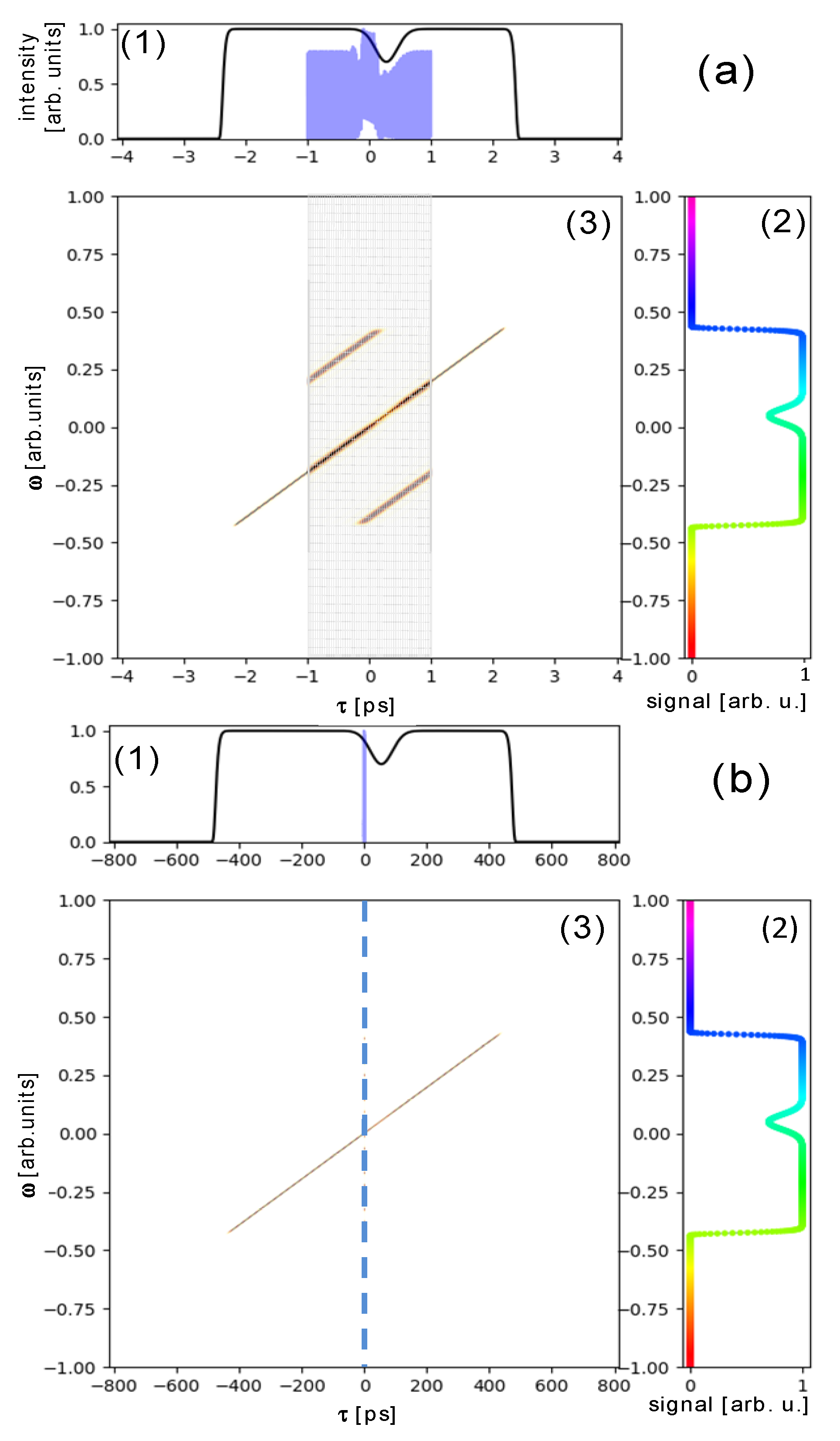
However, in a CPA laser, the pulse is stretched. Its time-bandwidth product rises to about 10⁵. The temporal excursion of the pulse is then greater than that used for the simulation, as shown by the grey grid in Figure 2a (3). By using Fourier transformation, such as in Wigner–Ville or spectrogram simulation, the temporal domain is restricted to this area. The simulation then presents temporal aliasing that is harmful to the result, as shown in Figure 2a (3), as well as by the blue curve in Figure 2a (1). For conventional large-scale CPA lasers, the initial temporal domain is so small that it becomes nearly invisible on the IFR (Figure 2b (3)). With a conventional Fourier transform, in order to avoid this temporal aliasing, the only solution is to proportionally increase the number of samples on both axes.

This makes it difficult to use Fourier transformations for very strongly stretched pulses with huge time-bandwidth products, as the required number of points grows quadratically alongside the stretching rate.

However, by using IFR, it is possible to stretch the temporal scale without restriction (Figure 2a,b), which makes the method very useful for large-stretched CPA laser pulses. This stretching corresponds to a translation of the points on the instantaneous curve, depending on the frequency in time. For each ω_i, the position of the new point is modified by the relative delay from the central pulsation:

$$\mathrm{d}\mathsf{\tau }\left({\mathsf{\omega }}_{\mathrm{i}}\right)={\left(\partial \mathsf{\phi }/\partial \mathsf{\omega }\right)}_{{\mathsf{\omega }}_{\mathrm{i}}-{\mathsf{\omega }}_0}.$$

(6)

The operation has no temporal limitation and does not need a regular temporal pattern. It is a pure line-by-line spectral operation. The output temporal scale is no longer linked to the spectral one by a regular point-to-point pattern. The temporal amplitude estimation will then require either resampling of the curve on a regular temporal pattern or consideration of the irregular pattern in the amplitude calculation. The IFR will then be compatible with any time-bandwidth product.

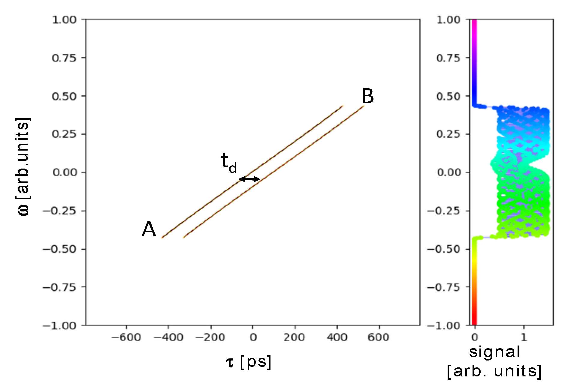
Pulse replicas are also due to linear operations but combine both spectral amplitude and spectral phase. As an example, a post-pulse delayed by t_d is simply introduced by replicating the IF curve and translating the full curve by t_d. Here, the absolute phase difference at ${\mathsf{\omega }}_0$ between the pulses is ignored. It can be considered by using an additional array within the phase values or by using complex weights rather than purely real ones. The calculation of the spectral amplitude is then more complex as it requires the integration of all the different ω_i components. The sum of these components includes the phase terms that are frequency dependent $\mathsf{\phi }\left({\mathsf{\omega }}_{\mathrm{i}}\right)={\mathsf{\omega }}_{\mathrm{i}}{\mathrm{t}}_{\mathrm{d}}$. The spectral amplitude is then obtained through the following integration:

$$\tilde{\mathrm{A}}\left({\mathsf{\omega }}_{\mathrm{i}}\right)={{\displaystyle \int }}_{-\mathrm{T}}^{\mathrm{T}}\mathrm{A}\left(\mathsf{\tau }\right){\mathrm{e}}^{{\mathrm{i}\mathsf{\omega }}_{\mathrm{i}}\mathsf{\tau }}\mathrm{d}\mathsf{\tau }.$$

(7)

By symmetry, the temporal intensity is also recovered by integration as:

$$\mathrm{A}\left({\mathsf{\tau }}_{\mathrm{i}}\right)={{\displaystyle \int }}_{-\infty }^{\infty }\tilde{\mathrm{A}}\left(\mathsf{\omega }\right){\mathrm{e}}^{{\mathrm{i}\mathsf{\omega }\mathsf{\tau }}_{\mathrm{i}}}\mathrm{d}\mathsf{\omega }.$$

(8)

As expected by its linear nature, this operation is still performed line by line (spectral amplitude) or column by column (temporal amplitude). Combining the main pulse with a post-pulse, generated, e.g., by partial internal reflection in planar transmission optics, and stretching results in what usually occurs in CPA systems (Figure 3).

Without nonlinearities, the pulses are then amplified with minor dispersions and minor spectral narrowing due to amplification. With proper dispersion management, the main pulse is perfectly recompressed by the compressor, and the output and input pulses look very similar to one another. PW-class CPA systems are designed to maximize the extracted laser pulse power, resulting in an operation close to or within an intensity range of the stretched pulse that causes significant nonlinearities. This results in laser pulse degradation that is deleterious for ultra-high laser applications. The main effect is the Kerr effect, globally characterized by the B-integral. The most deleterious impact of this effect on the temporal contrast is the pre-pulse generation from a post pulse by temporal diffraction [6,10,11].

Let us consider the two pulses of Figure 3, E₁ representing the main pulse and E₂ a post-pulse time, delayed by t_d. The third-order nonlinear polarization due to the Kerr effect [11] is

$${\mathrm{P}}_{\mathrm{NL}}\left(\mathsf{\tau }\right)={\mathsf{\chi }}_3\left[{\mathrm{E}}_1\left({\mathsf{\omega }}_1\left(\mathsf{\tau }\right)\right)+{\mathrm{E}}_2\left({\mathsf{\omega }}_2\left(\mathsf{\tau }\right)\right)\right]\left[{\mathrm{E}}_1^{*}\left(-{\mathsf{\omega }}_1\left(\mathsf{\tau }\right)\right)+{\mathrm{E}}_2^{*}\left(-{\mathsf{\omega }}_2\left(\mathsf{\tau }\right)\right)\right]\left[{\mathrm{E}}_1\left({\mathsf{\omega }}_1\left(\mathsf{\tau }\right)\right)+{\mathrm{E}}_2\left({\mathsf{\omega }}_2\left(\mathsf{\tau }\right)\right)\right],$$

(9)

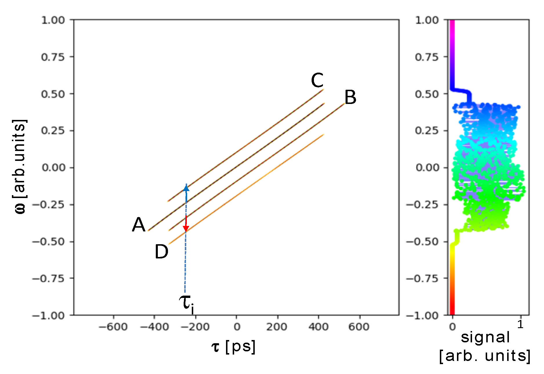
where it gives rise to four-wave mixing (FWM), self-phase modulation (SPM), cross-phase modulation (XPM) and cross-polarized wave generation (XPW). In particular, the terms ${\mathrm{E}}_1\left({\mathsf{\omega }}_1\left(\mathsf{\tau }\right)\right){\mathrm{E}}_2^{*}\left(-{\mathsf{\omega }}_2\left(\mathsf{\tau }\right)\right){\mathrm{E}}_1\left({\mathsf{\omega }}_1\left(\mathsf{\tau }\right)\right)$ and ${\mathrm{E}}_2\left({\mathsf{\omega }}_2\left(\mathsf{\tau }\right)\right){\mathrm{E}}_1^{*}\left(-{\mathsf{\omega }}_1\left(\mathsf{\tau }\right)\right){\mathrm{E}}_2\left({\mathsf{\omega }}_2\left(\mathsf{\tau }\right)\right)$ are the FWM processes of interest, giving the new frequencies 2${\mathsf{\omega }}_1-{\mathsf{\omega }}_2$, and 2${\mathsf{\omega }}_2-{\mathsf{\omega }}_1$. We see that a pre-pulse is generated t_d before the main pulse and ${\mathsf{\delta }\mathsf{\omega }}_1={\left(2{\mathsf{\omega }}_1-{\mathsf{\omega }}_2\right)}_{\mathsf{\tau }}-{\mathsf{\omega }}_1={\mathrm{bt}}_{\mathrm{d}},$ so it is constantly blue-shifted from ${\mathsf{\omega }}_1\left(\mathsf{\tau }\right)$ as b > 0 in PW-class CPA. Similarly, a post-pulse is also generated t_d after the post-pulse and ${\mathsf{\delta }\mathsf{\omega }}_2={\left(2{\mathsf{\omega }}_2-{\mathsf{\omega }}_1\right)}_{\mathsf{\tau }}-{\mathsf{\omega }}_2=-{\mathrm{bt}}_{\mathrm{d}}$ is red shifted from ${\mathsf{\omega }}_2\left(\mathsf{\tau }\right).$ Here, ${\mathsf{\delta }\mathsf{\omega }}_1$ indicates its origin from the main pulse ${\mathsf{\omega }}_1$, and ${\mathsf{\delta }\mathsf{\omega }}_2$ indicates its origin from the post-pulse ${\mathsf{\omega }}_2$. The FWM process is efficient as long as all spectral components are phase matched. The phase matching is kept since the components ${\mathsf{\omega }}_1\left(\mathsf{\tau }\right)$ and ${\mathsf{\omega }}_2\left(\mathsf{\tau }\right)$ are nearly equal. On the IFR, this temporal effect is simulated column by column. For any ${\mathsf{\tau }}_{\mathrm{i}}$, the temporal amplitude is calculated by using the inverse Fourier transform:

$$\forall {\mathsf{\tau }}_{\mathrm{i}},\mathrm{i}\in \left\{1..{\mathrm{N}}_{\mathsf{\tau }}\right\},\mathrm{A}\left(\mathrm{t},{\mathsf{\tau }}_{\mathrm{i}}\right)={\mathrm{FT}}^{-1}\left[\tilde{\mathrm{A}}\left(\mathsf{\omega },{\mathsf{\tau }}_{\mathrm{i}}\right)\right].$$

(10)

Then, the nonlinear effect is applied in this time domain:

$${\mathrm{A}}_{\mathrm{out}}\left(\mathrm{t},{\mathsf{\tau }}_{\mathrm{i}}\right)={\left|{\mathrm{A}}_{\mathrm{in}}\left(\mathrm{t},{\mathsf{\tau }}_{\mathrm{i}}\right)\right|}^2{\mathrm{A}}_{\mathrm{in}}\left(\mathrm{t},{\mathsf{\tau }}_{\mathrm{i}}\right).$$

(11)

Finally, the spectral amplitude at any ${\mathsf{\tau }}_{\mathrm{i}}$ is obtained by Fourier transform:

$$\forall {\mathsf{\tau }}_{\mathrm{i}},\mathrm{i}\in \left\{1..{\mathrm{N}}_{\mathsf{\tau }}\right\},\widetilde{{\mathrm{A}}_{\mathrm{out}}}\left(\mathsf{\omega },{\mathsf{\tau }}_{\mathrm{i}}\right)=\mathrm{FT}\left[{\mathrm{A}}_{\mathrm{out}}\left(\mathrm{t},{\mathsf{\tau }}_{\mathrm{i}}\right)\right].$$

(12)

The pre-pulse and post-pulse generation appears naturally from this process as shown in Figure 4.

If $\forall {\mathsf{\tau }}_{\mathrm{i}},\mathrm{i}\in \left\{1..{\mathrm{N}}_{\mathsf{\tau }}\right\},\mathrm{b}\left({\mathsf{\tau }}_{\mathrm{i}}\right)$ is large enough, then one can approximate: $\mathrm{A}\left(\mathrm{t},{\mathsf{\tau }}_{\mathrm{i}}\right)\approx \left[\frac{\tilde{\mathrm{A}}\left(\mathsf{\omega },{\mathsf{\tau }}_{\mathrm{i}}\right)}{\mathrm{b}\left({\mathsf{\tau }}_{\mathrm{i}}\right)}\right]$. Thus, $\widetilde{{\mathrm{A}}_{\mathrm{pre}-\mathrm{pulse}}}\left(\mathsf{\omega },{\mathsf{\tau }}_{\mathrm{i}}\right)\approx \mathsf{\alpha }{\left|\tilde{\mathrm{A}}\left(\mathsf{\omega },{\mathsf{\tau }}_{\mathrm{i}}\right)\right|}^2\widetilde{{\mathrm{A}}_{\mathrm{post}-\mathrm{pulse}}}\left(\mathsf{\omega },{\mathsf{\tau }}_{\mathrm{i}}\right)$, where $\mathsf{\alpha }$ is the coupling factor from post-pulse to pre-pulse [12].

3. Instantaneous Frequency Representation for a Realistic CPA Laser Simulation Step by Step

A typical CPA laser chain is depicted in Figure 5. Here, we follow the scheme presented by Liu et al. [11]. The pulses are derived from a high repetition rate mode-locked oscillator with an initial pulse length order of 25 fs. The laser pulse train typically passes Pockels cells, Faraday isolators and polarizers to decrease the repetition rate and for back-reflection isolation within the laser chain. The repetition rate is reduced for amplification to the order of a few Hz or less, especially in the case of petawatt class systems. After being stretched, typically from a time-bandwidth product of 0.5 to approximately 10⁵, or from 25 fs to 1ns, the laser pulse is amplified and recompressed close to the Fourier limit, which is determined by the spectral shape. The actively controlled spectral shape of the amplified pulse is typically a top hat, which is taken into account in all of the simulations presented here. Since the huge dispersion generated by the stretcher far outweighs the dispersion of the material in the amplifier chain, we only consider the stretcher and compressor as dispersive elements at this time.

Post-pulses are typically generated when the laser pulse passes through elements with plane-parallel surfaces. While for some cases this issue can be avoided by use of wedged components, causing spatio-temporal distortions and degrading the laser pulse quality in the focus, for others, this might not be possible. Anti-reflection coatings reduce the relative pulse level of the generated post-pulse to a certain degree. Plan-convex or plan-concave lenses can also cause post-pulses within a certain angular acceptance. For the simulation discussed here, we considered a rather large post-pulse level of 1% with respect to the main pulse and a delay of 100 ps.

Taking this into consideration, the spectral group delay can be expressed as:

$$\begin{array}{cc}\mathsf{\tau }\left(\mathsf{\omega }\right)& ={{\displaystyle \sum }}_{\mathrm{n}=2}^{\infty }\frac{{\mathsf{\phi }}_{\mathrm{n}}}{\left(\mathrm{n}-1\right)!}\left[{\left(\mathsf{\omega }-{\mathsf{\omega }}_0\right)}^{\mathrm{n}-1}\right] \approx {\mathsf{\phi }}_2\left(\mathsf{\omega }-{\mathsf{\omega }}_0\right)+\frac{{\mathsf{\phi }}_3}{2}{\left(\mathsf{\omega }-{\mathsf{\omega }}_0\right)}^2+\frac{{\mathsf{\phi }}_4}{3!}{\left(\mathsf{\omega }-{\mathsf{\omega }}_0\right)}^3\end{array}$$

(13)

where ${\mathsf{\phi }}_2$ is the linear chirp, mainly stretching the pulse and called the group velocity dispersion (GVD); ${\mathsf{\phi }}_3$ is the third-order spectral phase (third-order dispersion TOD), i.e., the first distortion order on the linear chirp; and ${\mathsf{\phi }}_4$ is the fourth-order spectral phase (fourth-order dispersion FOD), i.e., the second distortion order on the linear chirp. As sketched in Figure 5b, these distortions modify the previously used simplified IFR where only the linear chirp was applied, in contrast to Liu et al. [11].

The pulse and its post-pulse will undergo the Kerr-effect-induced FWM, which is predominantly induced by the amplifier materials [10]. After amplification, the pulses are recompressed by the compressor, such that the main pulse is near-perfect dispersion compensated and compressed as in the previous example.

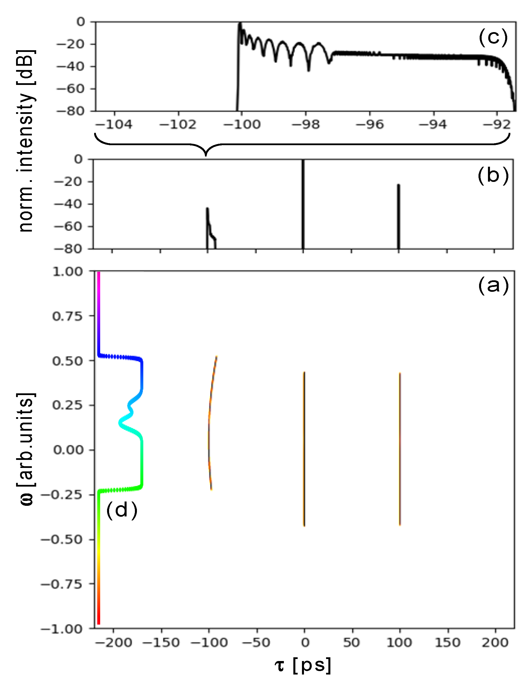
The first simulation considers only pure linear chirp stretching (Figure 6). The overall B-integral is chosen such that the pre-pulse generates yields close to the same power as the post-pulse [12], meaning about $\sqrt{3}$. As expected, in the output pulse, the Kerr effect through FWM generates a “time-diffracted” pre-pulse blue shifted in frequency. A post-pulse should also appear, but it is too weak to be visible on the dynamic scale of 80dB. In the ideal case of a pure chirp, as already mentioned by Liu et al. [11], the generated and compressed pre-pulse appears exactly with the mirrored delay of the original post-pulse but with significant frequency shifts (Figure 6a–c). This blue shift can be significant compared to the pulse bandwidth and can lead to an underestimated temporal deterioration by third-order cross-correlators with limited bandwidths [13]. The generated post-pulse can also be resolved on the temporal intensity display.

The simulation was performed on a standard personal computer with a 2000-point array in a few seconds without any code optimization. The chirp stretched the pulse by a factor of 40,000 (1ns stretched pulse), so the delay of 100 ps is still observable (Figure 3). Smaller or larger delays could be used without significant impact on simulation time and precision of the result.

In the more interesting case of distortions of the linear chirp, commonly present in the CPA stretcher and compressor realizations, the generated pre-pulse is modified and not recompressed completely at the output by the compressor. In the case of third-order spectral phase distortions, the pre-pulse is chirped (Figure 7) and its peak power can be decreased by two orders of magnitude. In contrast, the generated post-pulse appears unaffected, changing the relative pulse height of the pre- and post-pulse. The apparent delay of the pre-pulse is also shifted to a smaller delay than the equivalent delay of the post-pulse by symmetry.

For a fourth-order spectral phase distortion, the pre-pulse exhibits a third-order spectral phase distortion (Figure 8). Its maximum peak power is also decreased but less than for the third-order distortion. The generated post-pulse disappears below −80 dB. In both cases, interestingly, the peak power of the pre-pulse is decreased by the stretching and detuning of the pure linear chirp.

This pre-pulse temporal intensity distortion is similar to the one observed by Kiriyama et al. [6]. A proper stretching distortion could thus be intentionally applied to decrease the pre-pulse peak power and enhance the temporal contrast of the laser. This observation can be understood by the effect of the blue shift on the compression. Without the blue shift, the compressor fully compensates for the dispersion of the system. With the blue shift, the compensation is incomplete:

$$\begin{array}{ll}{\mathsf{\delta }\mathsf{\tau }}_{{\mathsf{\delta }\mathsf{\omega }}_1}\left(\mathsf{\omega }\right)& ={{\displaystyle \sum }}_{\mathrm{n}=2}^{\infty }\frac{{\mathsf{\phi }}_{\mathrm{n}}}{\left(\mathrm{n}-1\right)!}\left[\begin{array}{c}{\left(\mathsf{\omega }-{\mathsf{\omega }}_0\right)}^{\mathrm{n}-1}\\ -{\left(\mathsf{\omega }+{\mathsf{\delta }\mathsf{\omega }}_1-{\mathsf{\omega }}_0\right)}^{\mathrm{n}-1}\end{array}\right]\\ & ={{\displaystyle \sum }}_{\mathrm{n}=2}^{\infty }\frac{{\mathsf{\phi }}_{\mathrm{n}}}{\left(\mathrm{n}-1\right)!}\left(-{\mathsf{\delta }\mathsf{\omega }}_1\right)\left[{{\displaystyle \sum }}_{\mathrm{k}=0}^{\mathrm{n}-2}{{\displaystyle \sum }}_{\mathrm{j}=0}^{\mathrm{k}}\left(\begin{array}{c}\mathrm{k}\\ \mathrm{j}\end{array}\right){\left({\mathsf{\delta }\mathsf{\omega }}_1\right)}^{\mathrm{j}}{\left(\mathsf{\omega }-{\mathsf{\omega }}_0\right)}^{\mathrm{k}}\right]\end{array}$$

(14)

If we consider the effect nearby ${\mathsf{\omega }}_0$, $\mathsf{\omega }-{\mathsf{\omega }}_0\ll {\mathsf{\delta }\mathsf{\omega }}_1$ and that ${\mathsf{\delta }\mathsf{\omega }}_1$ is nearly constant over the bandwidth, the Nth-order distortion for the pre-pulse is produced by a combination of higher order terms of the stretcher dispersion:

$${\mathsf{\phi }}_{\mathrm{M},\mathrm{prepulse}}\left({\mathsf{\omega }}_0\right)=-{{\displaystyle \sum }}_{\mathrm{n}=\mathrm{M}+1}^{\infty }\frac{{\mathsf{\phi }}_{\mathrm{n}}}{\left(\mathrm{M}-1\right)!\left(\mathrm{n}-\mathrm{M}\right)!}{\left({\mathsf{\delta }\mathsf{\omega }}_1\right)}^{\mathrm{n}-\mathrm{M}}$$

(15)

For pure third-order distortion, the chirp of the pre-pulse can be approximated to:

$$\frac{\partial {\mathsf{\delta }\mathsf{\tau }}_{{\mathsf{\delta }\mathsf{\omega }}_1}\left(\mathsf{\omega }\right)}{\partial \mathsf{\omega }}\approx -\left[\left({\mathsf{\phi }}_3{\mathsf{\delta }\mathsf{\omega }}_1\right)\right].$$

(16)

For pure fourth order, the chirp is combined with a third order:

$$\frac{\partial {\mathsf{\delta }\mathsf{\tau }}_{{\mathsf{\delta }\mathsf{\omega }}_1}\left(\mathsf{\omega }\right)}{\partial \mathsf{\omega }}\approx -\left[\left(\frac{{\mathsf{\phi }}_4}{2!}{\mathsf{\delta }\mathsf{\omega }}_1{}^2\right)\right]-\left[\frac{{\mathsf{\phi }}_4}{2!}{\mathsf{\delta }\mathsf{\omega }}_1\right]\left[\left(\mathsf{\omega }-{\mathsf{\omega }}_0\right)\right].$$

(17)

These approximations confirm the effects seen in Figure 7 and Figure 8. Non-intuitively, having a large third order may ease the constraints on the pulse contrast, as it decreases the peak power of the generated pre-pulse due to its residual chirp. Note, however, that this model lacks precision because it assumes that ${\mathsf{\delta }\mathsf{\omega }}_1={\left({\mathsf{\omega }}_1-{\mathsf{\omega }}_2\right)}_{\mathsf{\tau }}$ is constant.

This realistic example of a case that is currently limiting high-intensity laser performance on the target illustrates the main advantage of the presented IFR simulation method. It is compatible with huge time-bandwidth product pulses existing in most high-power CPA laser systems. The temporal domain can be stretched and recompressed without loss of information and without any modification on the frequency domain. It is also very efficient numerically, as all the operations presented above are purely along one dimension.

4. Conclusions

We introduced a novel method for the simulation of nonlinearities on very large time-bandwidth product pulses. This method is very efficient numerically and is intuitive in the interpretation of the physical meaning of pulse modifications. It was applied to model pre-pulse generation in CPA chains as an example of current interest and will be used for a quantitative description of a full laser chain. Based on the investigated principles, it was observed in the simplified picture of single higher order stretching distortions that a contrast enhancement, i.e., a reduction in the intensity of the generated pre-pulse, becomes possible due to its corresponding incomplete compression.