Reactive Planning-Driven Approach to Online UAVs Mission Rerouting and Rescheduling

Abstract

The presented problem concerns the route planning of a UAV fleet carrying out deliveries to spatially dispersed customers in a highly dynamic and unpredictable environment within a specified timeframe. The developed model allows for predictive (i.e., taking into account forecasted changing weather conditions) and reactive (i.e., enabling contingency UAVs rerouting) delivery mission planning (i.e., NP-hard problem) in terms of the constraint satisfaction problem. Due to the need to implement an emergency return of the UAV to the base or handling ad hoc ordered deliveries, sufficient conditions have been developed. Checking that these conditions are met allows cases to be eliminated if they do not guarantee acceptable solutions, thereby allowing the calculations to be sped up. The experiments carried out showed the usefulness of the proposed approach in DSS-based contingency planning of the UAVs’ mission performed in a dynamic environment.

1. Introduction

In this paper, we consider the planning of the fleet mission problem for UAVs with highly dynamic and unpredictable environment constraints [1,2,3,4,5]. Typical disruptions in deliveries by UAVs may be caused by ad hoc changes to the deliveries ordered or changing weather conditions, which affect the energy consumption of UAVs and result in their shorter range due to the depletion of batteries [6,7]. For this reason, routing and scheduling a UAV fleet in partially known and unpredictable environments should take into account both projected changes in orders and weather conditions and selected categories of interference not included in previous forecasts. In other words, the planning of the UAVs’ missions should take into account the possibility of implementing both proactive (e.g., taking into account the projected disturbances) and reactive (e.g., enabling contingency reactions) behaviour.

UAV routes can be determined through proactive planning [6] and generated in an offline mode or in reactive planning [8,9] while executed in an online mode. Routes determined in proactive planning guarantee the achievement of the planned mission’s goal in terms of environmental parameters, which change at predetermined intervals. Scenarios corresponding to planned reactive rules do not guarantee reactive end-to-end paths employed in the routing process while adapting to changes in the environment during the execution of a mission [7,9,10,11,12,13,14,15,16]. In particular, the reactive routing strategies linking “route discovery” (proactive route planning) and “route maintenance” (adopting reactive rules) concepts [17] are responsible for the robustness of UAVs in terms of the changes in weather conditions. In this context, our study focuses on reactive planning [18,19] of deliveries by the UAVs’ fleet that are resistant to sudden atmospheric changes, resulting in a change in wind direction and intensity, rain or snow, precipitation, or unforeseen changes in delivery schedules caused by the cancellation of ordered deliveries or the notification of new orders.

In this context, the studies presented are a continuation of the previously published work focused on methods for planning UAVs’ fleet missions online [20,21]. Previous research has focused on selected planning strategies for UAVs’ fleet missions. These focus on arbitrarily chosen decomposition concepts for planned volumes of deliveries being phased out under submissions and are responsible for the partial distribution of supplies. Both variable weather conditions and ad hoc changing conditions for the volume of planned deliveries are taken into account. The aim of the research was to develop methods of predictive and/or reactive planning of acceptable options successively implemented under the supply of sub-missions, in particular the methods that enable their online use.

The originality of the paper results from merging the proactive and reactive planning of UAV fleet missions. The developed model allows for predictive (i.e., taking into account forecasted weather conditions changing) and reactive (i.e., enabling the interruption of a drone’s mission) planning for delivery missions in terms of the constraint satisfaction problem (CSP). This is easily implemented and commercially available in a constraint programming environment, e.g., IBM ILOG. In particular, the conditions guaranteeing the resistance function convexity, which consequently speed up the calculations (involved in the CSP solution) for the extended version of the UAVs’ mission planning are developed (i.e., taking into account multiple depots).

To summarise, the main objective of this paper is to introduce constraint programming based on a hybrid model. This is a combination of proactive and reactive planning and routing the UAVs’ fleet delivery missions. The new contributions provided to the currently available literature are (i) presenting a resistance function determining the UAVs’ mission resistance to both changes in weather conditions and changes to the times and location of deliveries, (ii) demonstrating the condition guaranteeing convexity of the resistance function in the polar coordinate system and (iii) conducting computational experiments confirming the usefulness of the proposed approach (i.e., the model and the condition based on it) for online planning of the UAVs’ fleet missions.

In other words, the proposed approach supports the decision-makers in their search for a plan of the missions (with routes and flight schedules), which allows for the delivery of an expected quantity of goods to a specific group of recipients. Introducing a new measure of the UAVs’ mission resistance and the analysis of the conditions guaranteeing its convexity allowed us to develop a declarative model of proactive/reactive UAV mission planning. Its computer implementation enables us to solve problems of scale encountered in practice online (distribution of goods for up to 90 customers). The remainder of this paper is organised as follows: Section 2 elaborates on related research. Section 3 presents the methodology used in the approach to UAV mission contingency planning. Section 4 describes the mathematical formulation for the declarative model for reactive planning of deliveries by the UAV fleet in terms of the constraint satisfaction problem. In Section 5, we focus on the relaxation of the convex resistance function aimed at developing restrictions, reducing the time-consuming assessment of weather conditions. Section 6 presents experiments that have been carried out and elaborates on the results obtained. Finally, Section 7 provides the final conclusions followed by a description of future research.

2. Related Work

A great number of publications are devoted to the study of various aspects of the construction [22,23,24] and operation [1,4,5,12,14] of UAVs and the possibilities for their use in various areas of civil missions (real-time monitoring, surveillance, reconnaissance, search and rescue) [25,26,27] and military areas (weapons delivery, guided missile support, directing artillery, spotting enemy positions). These publications also look at the methods for planning their missions [28]. The trend of research dedicated to online planning missions carried out by UAV teams has become increasingly noticeable. Research conducted in this area is devoted to the application of UAVs in emergency situations where they are used for transport of much-needed water, food, and medical supplies over hazardous (flooded) terrain. This is required due to climate change [29], necessitating the introduction of online UAV mission planning systems [20]. Other studies conducted in this area are devoted to various fields of application, e.g., reconnaissance and mapping [17], package delivery [3], delivery communication capabilities [22], healthcare [24,25], and so on. Increasing interest in these kinds of issues follows on from a need to search for scenario-driven planning methods that are aimed at the preparation of plans for UAV missions and aimed at an interactive tool building that facilitates the analysis and comparison of different scenarios and an iterative identification of sound and efficient mitigation strategies.

In the considered research domain, two directions can be distinguished. The first focuses on planning methods, taking into account weather uncertainty (e.g., investigating the manner in which energy consumption in UAV deliveries is affected by windy environmental conditions), and searching for route planning methods resistant to ad hoc changes in procurement conditions (e.g., studying the impact of changes in order terms and volumes to complete the planned delivery mission) [6,7,11]. In turn, the second research direction deals with methods of design and utilising networks of autonomous UAVs with complementary sensing and actuation equipment to collectively perform complicated tasks, i.e., the flying ad-hoc network (FANET) [30]. FANET spontaneously forms when UAVs connect and communicate with each other to facilitate long range missions and can be seen as a temporary type of local area network.

Indicated research gaps have become an inspiration for conducting this study, focusing on hybrid planning, i.e., a combination of proactive and reactive planning of the UAVs’ fleet delivery missions resistant to sudden changes in weather conditions and unforeseen changes in the arrangements for governing delivery schedules. To clarify the motivation standing behind the selection of the hybrid routing mode, we should note that the routes determined in proactive planning guarantee the achievement of the planned mission goal within the environment’s parameters, including change in predetermined intervals. In turn, routes determined in proactive planning guarantee the achievement of the mission goal only in the event of a previously foreseen (pre-planned) occurrence of an assumed type of disturbance. This is because a number of reactive rules guaranteeing the existence of reactive end-to-end paths employed in the routing process scenario is limited to just few arbitrarily chosen environmental changes.

In this context, this study proposes a novel model for proactive and reactive planning (different scenarios) that allow for a higher degree of realism, thus a higher likelihood of a mission being executed according to plan even when weather forecasts, order terms, and volumes to complete the planned delivery are changing. The novelty of this study results in the addition of a function of UAVs mission resistance to changes in weather conditions. In this context, we consider online re-planning when disturbances appear (e.g., earlier return of some of the UAVs from the fleet to the base), which exceeds the values incorporated at the proactive planning stage. The challenge in solving these types of problems is high computational complexity limiting solutions to small-scale problems. The ongoing work is focused on building models that enable the time-efficient planning of systems that are weatherproof and resistant to all kinds of UAV mission disturbances. To the best of our knowledge, it is the first model for solving a problem with the above-mentioned properties. The presented problem has been neither previously addressed nor solved in the existing literature [8,9,10,17,28,31,32,33,34], thus it is not possible to compare it directly with existing methods. The novelty of the presented approach results from the extension of the declarative model used in our previous works, particularly in [6,7,20,21] by the addition of a function of the UAVs mission resistance to both changes in weather conditions and changes in the times and locations of deliveries. The condition that constitutes this extension allows the UAV’s battery depletion to be foreseen in online mode before completing its mission, and thus it can be used in DSS-based planning of the UAVs’ fleet mission.

3. Approach to UAV Fleet Online Routing

We consider a distribution network, that is modelled by the graph $G=\left(N,E\right)$ where $N=\left\{N_1,\dots ,N_{\lambda },\dots ,N_n\right\}$ signifies the set of $n=\left|N\right|$ nodes and $E=\left\{\left(N_{\beta }, N_{\lambda }\right)|\beta ,\lambda \in \left\{1,\dots ,n\right\},\beta \ne \lambda \right\}$ signifies the set of edges determining the possible connections between nodes. Set $NB\subset N$ contains the nodes representing the bases and a set of $ND\subset N$ contains the nodes representing delivery points: $NB{{\displaystyle \cup }}^{ }ND=N$, $NB{{\displaystyle \cap }}^{ }ND=\varnothing$. Given a fleet of UAVs $\mathcal{U}=\left\{U_1,\dots ,U_k,\dots ,U_K\right\}$ that delivers goods to the points $ND$, the fleet $\mathcal{U}$ is spread between the bases $NB$, the subset ${\mathcal{U}}^{\lambda }\subseteq \mathcal{U}$ determines the UAVs allocated at base $N_{\lambda }\in NB$. An ordered quantity of goods $z_{\lambda }\in \mathbb{N}$(taken from the base $N_1$) should be transported to each delivery point $N_{\lambda }\in ND$. Deliveries are made as part of the mission S, which consists of sub-missions ${}_{ }{}^{l}S$ (i.e., delivery plans that include a single course of UAVs: base-delivery points-base). $Z$denotes a sequence consisting of variables $z_{\lambda }$: $Z$ $=(z_1,\dots ,z_n$) where $z_{\lambda }=0$ for each $N_{\lambda }\in NB$. It is assumed that all required goods should be delivered in the given horizon time $H$. The amount of goods delivered during one sub-mission ${}_{ }{}^{l}S$ by the $U_k$ to the delivery point $N_{\lambda }\in ND$ is determined by the variable ${}_{ }{}^{l}c{}_{\lambda }^k\in \mathbb{N}$. ${}_{ }{}^{l}C$ is a sequence$:$ ${}_{ }{}^{l}C=\left({}_{ }{}^{l}c{}_1^1,\dots ,{}_{ }{}^{l}c{}_1^K,\dots ,{}_{ }{}^{l}c{}_n^1,\dots ,{}_{ }{}^{l}c{}_n^K\right)$ determining the payload weight delivered by fleet $\mathcal{U}$ (${}_{ }{}^{l}c{}_{\lambda }^k=0$ for each $N_{\lambda }\in NB$). Variable $Q_k$ denotes the payload capacity of $U_k$ (amount of goods transported by $U_k$ cannot exceed $Q_k$). Moreover, each $U_k$ is described by the following technical parameters: the battery capacity $CAP$, airspeed $va$, drag coefficient $C_D$, front surface $A$, and UAV width $b$. The time spent on take-off and landing $U_k$on the delivery point $N_{\lambda }$ is indicated by variable $w_{\lambda }\in \mathbb{N}$. Note that ${}_{ }{}^l\mathcal{U}\subseteq \mathcal{U}$ denotes a set of UAVs used during sub-mission ${}_{ }{}^{l}S$. The time when the $U_k\in {}_{ }{}^l\mathcal{U}$ arrives at the delivery point $N_{\lambda }$ during a sub-mission ${}_{ }{}^{l}S$ is indicated by the variable ${}_{ }{}^{l}y{}_{\lambda }^k\in \mathbb{N}$ [s]. In this context, the sequence ${}_{ }{}^{l}Y$ consisting of moments ${}_{ }{}^{l}y{}_{\lambda }^k$ is called the schedule of the fleet ${}_{ }{}^l\mathcal{U}$: ${}_{ }{}^{l}Y=\left({}_{ }{}^{l}y{}_1^1,\dots ,{}_{ }{}^{l}y{}_1^K,\dots ,{}_{ }{}^{l}y{}_n^1,\dots ,{}_{ }{}^{l}y{}_n^K\right)$.

We assume that the variable $t_{\beta ,\lambda }\in \mathbb{N}$determines travelling time between nodes $N_{\beta }$,$N_{\lambda }$, where $\left(N_{\beta },N_{\lambda }\right)\in E$, and routes of $U_k\in {}_{ }{}^l\mathcal{U}$ during sub-mission ${}_{ }{}^{l}S$ are represented by the sequences ${}_{ }{}^l\pi {}_k=\left(N_{k_1},\dots ,N_{k_i},N_{k_{i+1}},\dots ,N_{k_{\mu }}\right)$, where $k_i\in \left\{1,\dots ,n\right\}$, $\left(N_{k_i},N_{k_{i+1}}\right)\in E$. ${}_{ }{}^l\Pi$ denotes a sequence of UAV routes executed during the sub-mission ${}_{ }{}^{l}S$: ${}_{ }{}^l\Pi =\left({}_{ }{}^l\pi {}_1,\dots ,{}_{ }{}^l\pi {}_k,\dots ,{}_{ }{}^l\pi {}_K\right)$ (in case when $U_k\notin {}_{ }{}^l\mathcal{U}$ then ${}_{ }{}^l\pi {}_k = △$). The delivery plan of one UAV’s sub-mission ${}_{ }{}^{l}S$ is defined as a sequence: ${}_{ }{}^{l}S=\left({}_{ }{}^l\mathcal{U},{}_{ }{}^l\Pi ,{}_{ }{}^{l}Y,{}_{ }{}^{l}C\right)$.

It is assumed that a plan of the UAVs’ sub-missions ${}_{ }{}^{l}S$ is implemented under specific weather conditions, i.e., the weather forecast is known for each sub-mission ${}_{ }{}^{l}S$. The forecasted weather conditions are described by the set $\mathbb{F}$ of pairs composed of direction $\theta$ and wind speed $vw$ $\left(\theta ,vw\right)\in \mathcal{F}$, i.e., $\mathbb{F}$ is defined as follows: $\mathbb{F}=\left\{\left(\theta ,vw\right)|\theta \in \left[0°,360°\right),vw\in \left[0, \mathcal{F}\left(\theta \right)\right]\right\}$. Where $Z\left(\theta \right)$ is a function whose values determine the maximum forecasted wind speed for a given direction $\theta$. The weather conditions determine the admissibility of the adopted sub-mission’s plan ${}_{ }{}^{l}S$, i.e., they determine whether the batteries of UAVs will be prematurely discharged during implementation.

A function ${{\rm Y}}_{k,l}\left(\theta \right)$ determines the borderline wind speed (for a given direction $\theta$), which guarantees the successful completion of the delivery plan by the $U_k$ during the sub-mission ${}_{ }{}^{l}S$ in the distribution network $G$: ${{\rm Y}}_{k,l}\left(\theta \right)=\max {\mathsf{\Gamma }}_{k,l}\left(\theta \right)$, where ${\mathsf{\Gamma }}_{k,l}\left(\theta \right)$—the set of the wind speed’s values $vw$ for a given direction $\theta$, for which the batteries of $U_k$ are not discharged. The sub-mission’s plan ${}_{ }{}^{l}S$ is assumed [12] to be resistant to the forecast weather conditions, $\mathbb{F}$, if the boundary wind ${{\rm Y}}_{k,l}\left(\theta \right)$ of all $U_k\in {}_{ }{}^l\mathcal{U}$ in any direction $\theta$ does not exceed the forecasted value $Z\left(\theta \right)$: ${\forall }_{U_k\in {}_{ }{}^l\mathcal{U}}{\forall }_{\theta \in \left[0°,360°\right)}{{\rm Y}}_{k,l}\left(\theta \right)\ge \mathcal{F}\left(\theta \right).$ The implementation of the designated mission S may be subject to various disturbances $IS$.

Among them, there are sudden changes in the weather (beyond the expected ${\mathcal{F}}^{*}\left(\theta \right)$ range and changes in orders $Z$), order changes (increased/decreased amount of ordered deliveries$Z^{*}$), changes to the number of delivery points served (changing the structure of the network $G^{*}$). The UAVs’ fleet, when performing the mission plan $S$, meets a disturbance $IS\left(t^{*}\right)$—covering one of the cases: the weather ${\mathcal{F}}^{*}\left(\mathsf{\theta }\right)$, the network $G^{*}$, orders ${\mathrm{Z}}^{*}$, the time $t^{*}.$ In such situations, it becomes necessary to answer to the question: Does a re-route plan exit for mission $S^{*}$ that guarantees timely deliveries in a given time horizon $H$ and at acceptable battery levels?

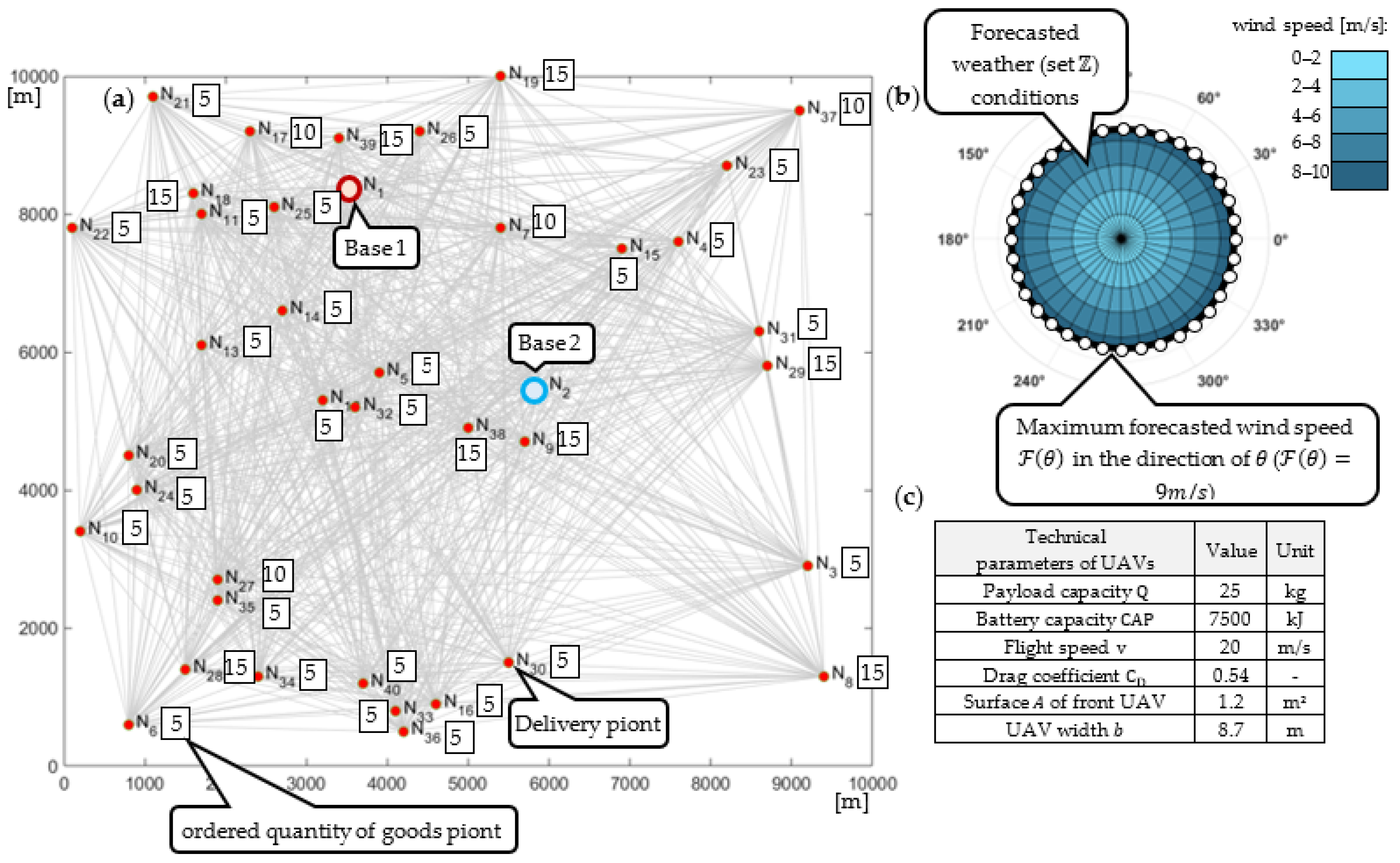
In order to provide an example to illustrate the proposed approach, let us consider a distribution network (from Figure 1a) covering an area of 100 km² and containing two bases, $NB=\left\{N_1,N_2\right\},$ and 38 delivery points $ND=\left\{N_3,\dots ,N_{40}\right\}$. The goods are delivered by a fleet of 4 UAVs ($\mathcal{U}=\left\{U_1,\dots ,U_4\right\}$) divided into two sub-fleets (${\mathcal{U}}^1=\left\{U_1,U_2\right\}$ and ${\mathcal{U}}^2=\left\{U_3,U_4\right\})$ serving the bases $N_1$ and $N_2$, respectively. The technical parameters of the UAVs are shown in the table in Figure 1c. The weight of individual orders is: ${\mathrm{z}}_3÷{\mathrm{z}}_6=5,{ \mathrm{z}}_7=10,{\mathrm{z}}_8={\mathrm{z}}_9=15,{ \mathrm{z}}_{10}÷{\mathrm{z}}_{16}=5,{ \mathrm{z}}_{17}=10$, ${\mathrm{z}}_{18}={\mathrm{z}}_{19}=15,{ \mathrm{z}}_{20}÷{\mathrm{z}}_{26}=5,{ \mathrm{z}}_{27}=10,{ \mathrm{z}}_{28}=15,{ \mathrm{z}}_{30}÷{\mathrm{z}}_{36}=5,{ \mathrm{z}}_{37}=10$, ${ \mathrm{z}}_{38}={\mathrm{z}}_{39}=15,{ \mathrm{z}}_{40}=5$. These assumptions are used to seek the UAVs mission $S$ plan guaranteeing timely deliveries (within the time horizon of 2.5 h) for the required amount of goods. The example of an admissible solution is presented in Figure 2. It consists of six sub-missions: $S=\left({}_{ }{}^{1}S,{}_{ }{}^{2}S,\dots ,{}_{ }{}^{6}S\right)$ following the wind speed constraints of <9 m/s.

An example illustrating the course of the UAVs fleet mission, ${}_{ }{}^{1}S$, and the values of the resistance functions, ${{\rm Y}}_{1,1}\left(\theta \right)$, ${{\rm Y}}_{2,1}\left(\theta \right)$, ${{\rm Y}}_{3,1}\left(\theta \right)$, ${{\rm Y}}_{4,1}\left(\theta \right)$, is shown in Figure 2. It is worth noting that the UAVs’ routing for mission ${}_{ }{}^{1}S$is weatherproof for a given weather forecast (i.e., ${{\rm Y}}_{k,l}\left(\theta \right)\ge \mathcal{F}\left(\theta \right)):$

$${}_{ }{}^1\mathsf{\pi }{}_1^{ }=\left({\mathrm{N}}_1,{ \mathrm{N}}_{14},{ \mathrm{N}}_6,{\mathrm{N}}_3,{\mathrm{N}}_{13},{ \mathrm{N}}_{11},{\mathrm{N}}_1\right); {}_{ }{}^1\mathsf{\pi }{}_2^{ }=\left({\mathrm{N}}_1,{\mathrm{N}}_{24},{\mathrm{N}}_{30},{\mathrm{N}}_{12},{\mathrm{N}}_{20},{\mathrm{N}}_{12},{\mathrm{N}}_1\right):$$

$${}_{ }{}^1\mathsf{\pi }{}_3^{ }=\left({\mathrm{N}}_2,{\mathrm{N}}_{32},{\mathrm{N}}_{40},{\mathrm{N}}_{26},{\mathrm{N}}_{22},{\mathrm{N}}_{23},{\mathrm{N}}_2\right); {}_{ }{}^1\mathsf{\pi }{}_4^{ }=\left({\mathrm{N}}_2,{\mathrm{N}}_5,{\mathrm{N}}_{31},{\mathrm{N}}_{36},{\mathrm{N}}_{12},{\mathrm{N}}_{15},{\mathrm{N}}_2\right)$$

All goods should be delivered within a time horizon not exceeding 2.5 h ($T=9000 \left[\mathrm{s}\right])$. The deliveries are made under various weather conditions (set $\mathbb{F}$), which are illustrated in Figure 1b. According to the forecast, the wind speed does not exceed $vw=9\frac{m}{s}$ in a direction of $\theta =0°–360°.$ Introducing of the additional base in node $N_2$ allows the delivery problem to be split into two sub-problems with one transportation network. As a result, this means that each base has its own unique parameters, e.g., the width of the time horizon for a given iteration, which can be overlapping. This approach can be used in real world applications, e.g., when two companies have the same transportation network, their own fleet of UAV’s, etc., they need to coordinate the transportation of goods between customers and avoid collisions.

We consider a situation in which the weather conditions of the mission carried out rapidly changed at the time $t^{*}=3000$ [s], i.e., during the execution of the sub-mission ${}_{ }{}^{2}S$, the wind speed increased to $vw = 11 \mathrm{m}/\mathrm{s}$ with the same intensity and direction $\theta =110°–130°$. Such a change means that this mission cannot be continued due to too much energy consumption (the mission’s resistance function ${{\rm Y}}_{3,2}\left(\theta \right)$ values are below the level corresponding to speed $11\frac{m}{s}$—see Figure 3). Figure 3 shows the location of the UAVs at time $t^{*}=3000 \left[\mathrm{s}\right]$, i.e., upon receipt of information about a change in weather and marking the place where the battery of $U_3$will be discharged in the event of continuation of deliveries in accordance with the current plan ${}_{ }{}^{2}S$.

In this situation, the route of the sub-mission ${}_{ }{}^{2}S$ being carried out needs to be corrected, requiring the below question to be answered.

Given a UAV fleet $\mathcal{U}=\left\{U_1,U_2,U_3,U_4 \right\}$ providing deliveries to the delivery points allocated in the network $G$ from Figure 1. The UAVs fleet carries out delivery mission plan $S^{*}$ from Figure 2. At the time $t^{*}=3000$, there is a sudden change in the weather conditions, i.e., disturbance $IS$ occurs, resulting in $vw = 11\frac{m}{s}$; $\theta =110°-130°$. This leads to a new question: Does a rerouting plan exist for mission $S^{*}$ that guarantees the timely delivery of the ordered supplies in a given time horizon $H=9000 \left[s\right]$ and at an acceptable battery level?

4. CSP Formulation

The proposed reaction to the occurrence of a disturbance $IS\left(t^{*}\right)$ can be reduced to dynamic re-routing and rescheduling of previously adopted routes ${}_{ }{}^l\Pi$, schedules ${}_{ }{}^{l}Y$ and delivered goods ${}_{ }{}^{l}C$ stated in the basic proactive plan for the mission by the UAVs’ fleet. This is a feasible adjustment of assumed ${}_{ }{}^l\Pi$, ${}_{ }{}^{l}Y,$ and ${}_{ }{}^{l}C$ values to the changes in forecasted weather ${\mathcal{F}}^{*}\left(\theta \right)$, and corrections introduced to the network $G^{*}$ or orders $Z^{*}$.

In order to formally define the concept of disturbance $IS\left(t^{*}\right),$ let us introduce the concept of the state of the mission’s implementation $S$. The state of the mission $S$ at the time $t$ is defined as follows: $IS\left(t\right)=\left(M\left(t\right), {\mathcal{F}}^{*}\left(\theta ,t\right),{}_{ }{}^{*}G\left(t\right),Z^{*}\left(t\right)\right)$ where $M\left(t\right)$ is an allocation of UAVs to nodes at the time $t$: ${}_{ }{}^{ }M\left(t\right)=\left(N_{a_1},\dots ,N_{a_k},\dots ,N_{a_K}\right)$, where $a_k\in \left\{1,\dots ,n\right\}$ determines the (delivery points) node $N_{a_k}$ occupied by $U_k$ (or the node the $U_k$ is headed to). ${\mathcal{F}}^{*}\left(\theta ,t\right)$ is the weather condition forecast at the time $t$. ${}_{ }{}^{*}G\left(t\right)$ is the graph model of the distribution network structure at time t (number and location of delivery points). $Z^{*}\left(t\right)$ is the sequence of goods requested at the time $t$. The state $IS\left(t^{*}\right)$ following condition $\left[{\mathcal{F}}^{*}\left(\theta ,t^{*}\right)\ne {\mathcal{F}}^{*}\left(\theta \right)\right]\vee \left[{}_{ }{}^{*}G\left(t^{*}\right)\ne G\right]\vee \left[Z^{*}\left(t^{*}\right)\ne Z\right]$ is called the disturbance occurring at the time $t^{*}$.

Occurrence of $IS\left(t^{*}\right)$ disturbance should be assessed in terms of its impact on the further course of the mission of S (that is, whether the value of the resistance function ${{\rm Y}}_{k,l}\left(\theta \right)$ is greater than$\mathcal{F}\left(\theta \right)$). If the implementation of the mission is at risk (${{\rm Y}}_{k,l}\left(\theta \right)\ngeqq \mathcal{F}\left(\theta \right)$), an attempt should be made to reschedule it. The following condition action (if-then) rules are used for this purpose:

1.

If the adopted mission plan $S$ is not resistant to disturbance $IS\left(t^{*}\right)$ $\left({\exists }_{\mathrm{k}\in \left\{1,\dots ,K\right\},\mathrm{l}\in \left\{1,\dots ,L\right\}}{{\rm Y}}_{k,l}\left(\mathsf{\theta }\right)\ngeqq \mathcal{F}\left(\mathsf{\theta }\right)\right),$a check should be carried out to see whether it is possible to adapt (re-plan) to the new conditions. That is, decide whether all UAVs in the air continue their current missions or make their appropriate corrections.

2.

If there are UAVs (the set $\mathcal{U}\mathrm{R}$) that cannot continue to fly due to disturbance $IS\left(t^{*}\right),$ then they should be returned to base, ensuring that airborne UAVs ($\mathrm{the} \mathrm{set} \mathcal{U}\backslash \mathcal{U}\mathrm{R}$) can take over their tasks.

3.

If the tasks of the UAVs returning to the base (the set $\mathcal{U}\mathrm{R})$ cannot be taken over by UAVs still performing their missions, a check should be carried out as to whether the reserve UAVs available at base (the set $\mathcal{U}\mathrm{B}$) can take over their responsibilities. This means the UAVs in the air continue their existing missions, while the reserve UAVs take over the liabilities of the UAVs returned to base.

4.

If the reserve UAVs (the set $\mathcal{U}\mathrm{B}$) are unable to take over the responsibilities returned to the base (the set $\mathcal{U}\mathrm{R}$), then their activity should be suspended until the disturbance is resolved.

The above rules have been used in the reactive mission planning method $S$. The idea behind this method is as follows: during the implementation of the mission $S$, there is a continuous monitoring of the state of the $IS\left(t\right)$ (for $t\in \left\{0\dots H\right\}$). If at the state $IS\left(t\right)$, the following condition holds $\left[{\mathcal{F}}^{*}\left(\theta ,t^{*}\right)\ne {\mathcal{F}}^{*}\left(\theta \right)\right]\vee \left[{}_{ }{}^{*}G\left(t^{*}\right)\ne G\right]\vee \left[Z^{*}\left(t^{*}\right)\ne Z\right]$ (i.e., there is a change in the weather forecast or in the structure of the distribution network, and the size of the requests, etc.) and the mission $S$ is under threat (i.e., at least one of the UAVs will not return to base due to low battery), then an attempt must be made to replan. This type of reaction is performed by the function solve, the purpose of which is to designate a mission ${}_{ }{}^{*}S$adapted to the new conditions determined by the disturbance $IS\left(t\right)$. In practice, it comes down to solving the relevant constraints satisfaction problem $CS\left({}_{ }{}^{\mathrm{O}}\mathcal{U},S, IS\left(t\right)\right)$ (where:${}_{ }{}^{\mathrm{O}}\mathcal{U}$ defines the fleet designated by condition action rules 1–4). The relevant constraints distribution process follows the sequence where at first an attempt is made to designate the mission ${}_{ }{}^{*}S$ for the fleet ${}_{ }{}^{➀}\mathcal{U}=\mathcal{U}$ (according to the rule 1). In the event of failure, an attempt is made to designate this for the fleet ${}_{ }{}^{➁}\mathcal{U}=\mathcal{U}\backslash \mathcal{U}R$ (according to rule 2) and then for the fleet ${}_{ }{}^{➂}\mathcal{U}=\left(\mathcal{U}\backslash \mathcal{U}R\right){{\displaystyle \cup }}^{ }\mathcal{U}B$ (according to rule 3). If an admissible solution ${}_{ }{}^{*}S$ still does not exist, then the mission plan currently used should be modified (due to the $\mathrm{reduce}$ function) in such a way that it removes the UAVs’ sub-missions that are not resistant to disturbance $IS\left(t\right)$ (according to rule 4).

It should be noted that the designation of mission ${}_{ }{}^{*}S$ is associated with the designation of routings ${}_{ }{}^l\Pi$, schedules ${}_{ }{}^{l}Y$ and delivery sequences ${}_{ }{}^{l}C$ throughout the remaining time horizon $\left\{t\dots H\right\}$. Due to the disturbance $IS\left(t^{*}\right)$ occurrence, the proposed reactive planning algorithm (implemented in the IBM ILOG environment) generates the end-to-end paths that modify previously planned routes, restoring the ability to implement the designated mission delivery plan.

The mathematical formulation of the constraint satisfaction problem $CS\left({}_{ }{}^{\mathrm{O}}\mathcal{U},S, IS\left(t\right)\right)$ aimed at contingency planning for the UAVs’ mission design employs the following parameters, variables, sets, and constraints:

Parameters:

${}_{ }{}^{l}G$	$\mathrm{the} \mathrm{graph} \mathrm{of} \mathrm{a} \mathrm{distribution} \mathrm{network} \mathrm{for} \mathrm{sub}-\mathrm{mission} {}_{ }{}^{l}S$,	${}_{ }{}^l\mathcal{U}$	$\mathrm{the} \mathrm{subset} \mathrm{of} \mathrm{UAVs} {}_{ }{}^l\mathcal{U}\subseteq \mathcal{U}$$\mathrm{carrying} \mathrm{out} \mathrm{the} \mathrm{sub}-\mathrm{mission} {}_{ }{}^{l}S$,
$z_{\lambda }$	$\mathrm{the} \mathrm{demand} \mathrm{at} \mathrm{node} N_{\lambda }$$, z_1=0$,	$K$	the size of the fleet of UAVs,
$d_{\beta ,\lambda }$	$\mathrm{the} \mathrm{distance} \mathrm{between} N_{\beta }$$, N_{\lambda }$,	$A$	the front-facing area of a UAV,
$t_{\beta ,\lambda }$	$\mathrm{the} \mathrm{travel} \mathrm{time} \mathrm{between} N_{\beta }$$, N_{\lambda }$,	$C_D$	the aerodynamic drag coefficient,
$w$	the time spent on take-off and landing of a UAV,	$ts$	the time interval at which UAVs can take off from the base,
$Q$	the maximum loading capacity,	$ep$	the empty weight of a UAV,
$IS\left(t\right)$	the state of UAV’s mission,	$D$	the air density,
$H$	the time horizon,	$g$	the gravitational acceleration,
${{\rm Y}}_{k,l}\left(\theta \right)$	the weather resistance function,	$b$	the width of a UAV,
$\mathcal{F}{\left(\theta \right)}^{ }$	the forecasted wind speed,	$CAP$	the energy capacity of a UAV,
$v{a}_{\beta ,\lambda }^{ }$	$\mathrm{the} \mathrm{air} \mathrm{speed} \mathrm{between} \mathrm{nodes} N_{\beta }$$, N_{\lambda }$,	$v{g}_{\beta ,\lambda }^{ }$	$\mathrm{ground} \mathrm{speed} \mathrm{between} N_{\beta }$$, N_{\lambda }$,
${\phi }_{\beta ,\lambda }$	$\mathrm{the} \mathrm{heading} \mathrm{angle} \mathrm{of} \mathrm{vector} v{a}_{\beta ,\lambda }^{ }$,	${\vartheta }_{\beta ,\lambda }$	$\mathrm{the} \mathrm{course} \mathrm{angle} \mathrm{of} \mathrm{vector} v{g}_{\beta ,\lambda }^{ }$,
$ND$	the set of delivery points,	$NB$	the set of bases,
${\mathcal{U}}^{\lambda }$	$\mathrm{the} \mathrm{set} \mathrm{of} \mathrm{UAVs} \mathrm{allocated} \mathrm{at} \mathrm{base} N_{\lambda }\in NB$,	${}_{ }{}^{l}y{}_{\lambda }^k$	$\mathrm{the} \mathrm{time} \mathrm{at} \mathrm{which} U_k$$\mathrm{arrives} \mathrm{at} \mathrm{node} N_{\lambda }$$, \mathrm{before} \mathrm{the} \mathrm{disturbance} IS\left(t^{*}\right)$ occurrence,
${}_{ }{}^{l}s{}^k$	$\mathrm{the} \mathrm{take}-\mathrm{off} \mathrm{time} \mathrm{of} U_k$$\mathrm{before} \mathrm{the} \mathrm{disturbance} IS\left(t^{*}\right)$,	${}_{ }{}^{l}x{}_{\beta ,\lambda }^k$	$\mathrm{the} \mathrm{binary} \mathrm{variable} \mathrm{used} \mathrm{to} \mathrm{indicate} \mathrm{whether} \mathrm{the} \mathrm{flight} \mathrm{between} \mathrm{points} N_{\beta }$$, N_{\lambda }$$, \mathrm{takes} \mathrm{place} \mathrm{before} \mathrm{the} \mathrm{disturbance} IS\left(t^{*}\right)$ occurs,
${}_{ }{}^{l}y{}_{\lambda }^k$	$\mathrm{the} \mathrm{time} \mathrm{at} \mathrm{which} U_k$$\mathrm{arrives} \mathrm{at} \mathrm{node} N_{\lambda }$$\mathrm{before} \mathrm{the} \mathrm{disturbance} IS\left(t^{*}\right)$,	${}_{ }{}^{l}c{}_{\lambda }^k$	$\mathrm{the} \mathrm{weight} \mathrm{of} \mathrm{freight} \mathrm{delivered} \mathrm{to} \mathrm{node} N_{\lambda }$$\mathrm{by} U_k$$, \mathrm{before} \mathrm{the} \mathrm{disturbance} IS\left(t^{*}\right)$ occurrence,

Decision Variables:

$\overline{{}_{ }{}^{l}x{}_{\beta ,\lambda }^k}$	$\mathrm{the} \mathrm{binary} \mathrm{variable} \mathrm{used} \mathrm{to} \mathrm{indicate} \mathrm{if} U_k$$\mathrm{travels} \mathrm{between} \mathrm{nodes} N_{\beta }$$, N_{\lambda }$$\mathrm{after} \mathrm{the} \mathrm{disturbance} IS\left(t^{*}\right)$$\mathrm{occurrence} (\mathrm{during} \mathrm{sub}-\mathrm{mission} {}_{ }{}^{l}S$),
	$\overline{{}_{ }{}^{l}x{}_{\beta ,\lambda }^k}=\{\begin{array}{cc}1& if U_k travels between nodes N_{\beta }, N_{\lambda }\\ 0& otherwise.\end{array}$
$\overline{{}_{ }{}^{l}y{}_{\lambda }^k}$	$\mathrm{the} \mathrm{time} \mathrm{at} \mathrm{which} U_k$$\mathrm{arrives} \mathrm{at} \mathrm{node} N_{\lambda }$$\mathrm{after} \mathrm{disturbance} IS\left(t^{*}\right)$$\mathrm{occurrence} (\mathrm{during} \mathrm{sub}-\mathrm{mission} {}_{ }{}^{l}S$),
$\overline{{}_{ }{}^{l}c{}_{\lambda }^k}$	$\mathrm{the} \mathrm{weight} \mathrm{of} \mathrm{freight} \mathrm{delivered} \mathrm{to} \mathrm{node} N_{\lambda }$$\mathrm{by} U_k$$\mathrm{after} \mathrm{the} \mathrm{disturbance} IS\left(t^{*}\right)$$\mathrm{occurrence} (\mathrm{during} \mathrm{sub}-\mathrm{mission} {}_{ }{}^{l}S$),
$\overline{{}_{ }{}^{l}f{}_{\beta ,\lambda }^k}$	$\mathrm{the} \mathrm{weight} \mathrm{of} \mathrm{freight} \mathrm{carried} \mathrm{between} \mathrm{nodes} N_{\beta }$$, N_{\lambda }$$\mathrm{by} U_k$$\mathrm{after} \mathrm{the} \mathrm{disturbance} IS\left(t^{*}\right)$$\mathrm{occurrence} (\mathrm{during} \mathrm{sub}-\mathrm{mission} {}_{ }{}^{l}S$),
$\overline{{}_{ }{}^{l}P{}_{\beta ,\lambda }^k}$	$\mathrm{the} \mathrm{energy} \mathrm{per} \mathrm{unit} \mathrm{of} \mathrm{time} \mathrm{consumed} \mathrm{by} U_k$$\mathrm{during} \mathrm{the} \mathrm{flight} \mathrm{between} \mathrm{nodes} N_{\beta }$$, N_{\lambda }$$(\mathrm{after} \mathrm{the} \mathrm{disturbance} IS\left(t^{*}\right)$ occurrence),
$\overline{{}_{ }{}^{l}ba{t}^k}$	$\mathrm{the} \mathrm{total} \mathrm{energy} \mathrm{consumed} \mathrm{by} U_k$$\mathrm{after} \mathrm{the} \mathrm{disturbance} IS\left(t^{*}\right)$$\mathrm{occurrence} (\mathrm{during} \mathrm{sub}-\mathrm{mission} {}_{ }{}^{l}S$),
$\overline{{}_{ }{}^{l}s{}^k}$	$\mathrm{the} \mathrm{take}-\mathrm{off} \mathrm{time} \mathrm{of} U_k$$\mathrm{after} \mathrm{disturbance} IS\left(t^{*}\right)$ occurrence,
$\overline{{}_{ }{}^{l}c{p}_{\lambda }}$	$\mathrm{the} \mathrm{total} \mathrm{weight} \mathrm{of} \mathrm{freight} \mathrm{delivered} \mathrm{to} \mathrm{node} N_{\lambda }$$\mathrm{after} \mathrm{the} \mathrm{disturbance} IS\left(t^{*}\right)$$\mathrm{occurrence} (\mathrm{during} \mathrm{sub}-\mathrm{mission} {}_{ }{}^{l}S$),
$\overline{{}_{ }{}^l\pi {}_k^{ }}$	$\mathrm{the} \mathrm{route} \mathrm{of} U_k$$\mathrm{after} \mathrm{the} \mathrm{disturbance} IS\left(t^{*}\right)$$\mathrm{occurrence} (\mathrm{during} \mathrm{sub}-\mathrm{mission} {}_{ }{}^{l}S$$), \overline{{}_{ }{}^l\pi {}_k}=\left(N_{k_1},\dots ,N_{k_i},N_{k_{i+1}},\dots ,N_{k_{\mu }}\right)$$, k_i\in \left\{1,\dots ,n\right\}$,$\left(N_{k_i},N_{k_{i+1}}\right)\in E$

Sets

$\overline{{}_{ }{}^{l}Y}$	$\mathrm{the} \mathrm{sequence} \mathrm{of} \mathrm{moments} \overline{{}_{ }{}^{l}y{}_{\lambda }^k}$$\mathrm{that} \mathrm{schedules} \mathrm{the} \mathrm{fleet} {}_{ }{}^l\mathcal{U}$$\mathrm{after} \mathrm{the} \mathrm{disturbance} IS\left(t^{*}\right)$ occurrence,
$\overline{{}_{ }{}^{l}C}$	$\mathrm{the} \mathrm{sequence} \mathrm{of} \mathrm{weights} \mathrm{of} \mathrm{delivered} \mathrm{goods} \overline{{}_{ }{}^{l}c{}_{\lambda }^k}$,
$\overline{{}_{ }{}^l\Pi }$	$\mathrm{the} \mathrm{set} \mathrm{of} \mathrm{UAV} \mathrm{routes} \overline{{}_{ }{}^l\pi {}_k^{ }}$,
${\overline{{}_{ }{}^{l}S}}_{ }$	$\mathrm{the} \mathrm{plan} \mathrm{of} \mathrm{sub}-\mathrm{mission} \mathrm{after} \mathrm{the} \mathrm{disturbance} IS\left(t^{*}\right)$$\mathrm{occurrence}: \overline{{}_{ }{}^{l}S}=\left({}_{ }{}^l\mathcal{U},\overline{{}_{ }{}^l\Pi },\overline{{}_{ }{}^{l}Y},\overline{{}_{ }{}^{l}C}\right)$,
	$\mathrm{the} \mathrm{re}-\mathrm{route} \mathrm{plan} \mathrm{of} \mathrm{the} \mathrm{mission} {}_{ }{}^{*}S=\left({\overline{{}_{ }{}^{1}S}}_{ },\dots ,{\overline{{}_{ }{}^{l}S}}_{ },\dots ,{\overline{{}_{ }{}^{L}S}}_{ }\right).$

Constraints: routes, delivery of freight, and energy consumption.

1.

Routes. Relationships between the variables describing UAV take-off times/mission start times and task order:

$$\overline{{}_{ }{}^{l}s{}^k}\ge 0; k=1\dots K, l=1\dots L$$

(1)

$$\overline{{}_{ }{}^{l}s{}^k}\ge 0; k=1\dots K, l=1\dots L,$$

(2)

$$\left(\left|\overline{{}_{ }{}^{l}s{}^k}-\overline{{}_{ }{}^{l}s{}^q}\right|\ge ts\right) ;\forall U_k, \forall U_q\in {\mathcal{U}}^{\lambda }, \forall N_{\lambda }\in NB, l=1\dots L,$$

(3)

$$\left( {}_{ }{}^{l}y{}_j^k\le t^{*}\right)\Rightarrow \left(\overline{{}_{ }{}^{l}x{}_{i,j}^k}={}_{ }{}^{l}x{}_{i,j}^k\right); j=1\dots n, i=1\dots n, k=1\dots K, l=1\dots L,$$

(4)

$$\left( {}_{ }{}^{l}y{}_j^k\le t^{*}\right)\Rightarrow \left(\overline{{}_{ }{}^{l}y{}_j^k}={}_{ }{}^{l}y{}_j^k\right); j=1\dots n;k=1\dots K, l=1\dots L,$$

(5)

$${{\displaystyle \sum }}_{j=1}^n\overline{{}_{ }{}^{l}x{}_{i,j}^k}=1 ; k=1\dots K, i=1\dots n, l=1\dots L,$$

(6)

$$\left(\overline{{}_{ }{}^{l}x{}_{\lambda ,j}^k}=1\right)\Rightarrow \left(\overline{{}_{ }{}^{l}y{}_j^k}=\overline{{}_{ }{}^{l}s{}^k}+t_{\mathsf{\lambda },j}\right) ; \forall N_j\in ND; \forall N_{\lambda }\in NB, U_k\in {\mathcal{U}}^{\lambda }, l=1\dots L$$

(7)

$$\left(\overline{{}_{ }{}^{l}y{}_{\lambda }^k}\ne 0 \wedge \overline{{}_{ }{}^{l}y{}_{\lambda }^q}\ne 0 \right)\Rightarrow \left(\left|\overline{{}_{ }{}^{l}y{}_{\lambda }^k}-\overline{{}_{ }{}^{l}y{}_{\lambda }^q}\right|\ge w\right) ; k,q=1\dots K; k\ne q; \forall N_{\lambda }\in ND$$

(8)

$$\left(\overline{{}_{ }{}^{l}x{}_{\lambda ,j}^k}=1\right)\Rightarrow \left(\overline{{}_{ }{}^{l}y{}_j^k}=\overline{{}_{ }{}^{l}y{}_{\lambda }^k}+t_{\lambda ,j}+w\right); \forall N_{\lambda }, \forall N_J\in ND; k=1\dots K,$$

(9)

$$\overline{{}_{ }{}^{l}y{}_i^k}\ge 0; i=1\dots n; k=1\dots K,$$

(10)

$${{\displaystyle \sum }}_{j=1}^n\overline{{}_{ }{}^{l}x{}_{i,j}^k}={{\displaystyle \sum }}_{j=1}^n\overline{{}_{ }{}^{l}x{}_{j,i}^k}; i=1\dots n; k=1\dots K,$$

(11)

$$\overline{{}_{ }{}^{l}y{}_i^k}\le H\times {{\displaystyle \sum }}_{j=1}^n\overline{{}_{ }{}^{l}x{}_{i,j}^k}, i=1\dots n; k=1\dots K,$$

(12)

$$\overline{{}_{ }{}^{l}y{}_i^k}\le H\times {{\displaystyle \sum }}_{j=1}^n\overline{{}_{ }{}^{l}x{}_{i,j}^k}, i=1\dots n; k=1\dots K,$$

(13)

2.

Delivery of freight. Relationships between variables describing freight quantities already delivered and requested

$$\left( \overline{{}_{ }{}^{l}y{}_j^k}\le t^{*}\right)\Rightarrow \left(\overline{{}_{ }{}^{l}c{}_j^k}={}_{ }{}^{l}c{}_j^k\right); j=1\dots n;k=1\dots K; l=1\dots L,$$

(14)

$$\overline{{}_{ }{}^{l}c{}_i^k}\ge 0; i=1\dots n; k=1\dots K;l=1\dots L,$$

(15)

$$\overline{{}_{ }{}^{l}c{}_i^k}\le Q\times {{\displaystyle \sum }}_{j=1}^n{x}_{i,j}^k; i=1\dots n; k=1\dots K, l=1\dots L,$$

(16)

$${{\displaystyle \sum }}_{i=1}^n\overline{{}_{ }{}^{l}c{}_i^k}\le Q; k=1\dots K;l=1\dots L,$$

(17)

$$\left(\overline{{}_{ }{}^{l}x{}_{i,j}^k}=1 \right)\Rightarrow \left(\overline{{}_{ }{}^{l}c{}_i^k}\ge 1\right); k=1\dots K; \forall N_i\in N; \forall N_j\in ND$$

(18)

$${{\displaystyle \sum }}_{l=1}^L{{\displaystyle \sum }}_{k=1}^K\overline{{}_{ }{}^{l}c{}_i^k}=z_i; \forall N_i\in ND ,$$

(19)

$${{\displaystyle \sum }}_{i=1}^n\overline{{}_{ }{}^{l}c{}_i^k}=\overline{{}_{ }{}^{l}c{s}^k}; k=1\dots K; l=1\dots L,$$

(20)

$$\left(\overline{{}_{ }{}^{l}x{}_{i,j}^k}=1\right)\Rightarrow \left(\overline{{}_{ }{}^{l}f{c}_j^k}=\overline{{}_{ }{}^{l}c{s}^k}\right) ;j=1\dots n; k=1\dots K, l=1\dots L,$$

(21)

$$\left(\overline{{}_{ }{}^{l}x{}_{i,j}^k}=1\right)\Rightarrow \left(\overline{{}_{ }{}^{l}f{c}_j^k}=\overline{f{c}_i^k}-\overline{{}_{ }{}^{l}c{}_i^k}\right) ;i,j=1\dots n; k=1\dots K, l=1\dots L,$$

(22)

$$\left(\overline{{}_{ }{}^{l}x{}_{i,j}^k}=1\right)\Rightarrow \left(\overline{{}_{ }{}^{l}f{}_{1,j}^k}=\overline{{}_{ }{}^{l}c{s}^k}\right) ;j=1\dots n; k=1\dots K, l=1\dots L,$$

(23)

$$\left(\overline{{}_{ }{}^{l}x{}_{i,j}^k}=1\right)\Rightarrow \left(\overline{{}_{ }{}^{l}f{}_{i,j}^k}=\overline{{}_{ }{}^{l}f{c}_j^k}\right) ; i,j=1\dots n; k=1\dots K, l=1\dots L,$$

(24)

3.

Energy consumption. In order to ensure the waterproof quality of the ${}_{ }{}^{l}S$ sub-mission (i.e., its robustness to weather condition changes $Z\left(\theta \right)$) the amount of energy required to complete the task carried out by a UAV must not exceed the capacity of its battery.

$${{\rm Y}}_{k,l}\left(\theta \right)\ge \mathcal{F}\left(\theta \right); \forall \theta \in \left[0^{\circ },{360}^{\circ }\right),$$

(25)

$${{\rm Y}}_{k,l}\left(\theta \right)=\max {\mathsf{\Gamma }}_{k,l}\left(\theta \right)$$

(26)

$${\mathsf{\Gamma }}_{k,l}\left(\theta \right)=\left\{vw | vw\in R_{+}^0\wedge \forall { }_{k\in \left\{1\dots K\right\}}\overline{{}_{ }{}^{l}ba{t}^k}\left(\theta ,vw\right)\le CAP\right\},$$

(27)

$$\overline{{}_{ }{}^{l}ba{t}^k}\left(\theta ,vw\right)={{\displaystyle \sum }}_{i=1}^n{{\displaystyle \sum }}_{j=1}^n\overline{{}_{ }{}^{l}x{}_{i,j}^k}\times t_{i,j}\times {}_{ }{}^{l}P{}_{i,j}^k\left(\theta ,vw\right),$$

(28)

$${}_{ }{}^{l}P{}_{i,j}^k\left(\theta ,vw\right)=\frac{1}{2}{C}_D\times A\times D\times {\left(v{a}_{i,j}^{ }\left(\theta ,vw\right)\right)}^3+\frac{{\left(\left(ep+\overline{{}_{ }{}^{l}f{}_{i,j}^k}\right)\times \mathrm{g}\right)}^{\frac{3}{2}}}{\sqrt{2\times D\times A}},$$

(29)

where ${}_{ }{}^{l}v{a}_{i,j}^{ }\left(\theta ,vw\right)$ and $t_{i,j}$ depend on the assumed goods delivery strategy, $D$ is an air density that is equal to 1.225 kg/m³, and $A$ is the front-facing area of UAV that is equal to 1.2 m² (provided by the UAV manufacturer).

If the ground speed $v{g}_{i,j}^{ }$ is constant, then an air speed ${}_{ }{}^{l}v{a}_{i,j}^{ }$ is calculated from:

$${}_{ }{}^{l}v{a}_{i,j}^{ }\left(\theta ,vw\right)=\sqrt{{\left(v{g}_{i,j}^{ }\times cos{\vartheta }_{i,j}-vw\times cos{\theta }_{ }\right)}^2+{\left(v{g}_{i,j}^{ }\times sin{\vartheta }_{i,j}-vw\times sin{\theta }_{ }\right)}^2}$$

(30)

$$t_{i,j}=d_{i,j}/v{g}_{i,j}^{ }$$

(31)

Since the re-planning of the mission delivery plan. S, is the result of the disturbance, $IS\left(t^{*}\right)$, the new set of sub-missions ${\overline{{}_{ }{}^{1}S}}_{ },\dots ,{\overline{{}_{ }{}^{l}S}}_{ },\dots ,{\overline{{}_{ }{}^{L}S}}_{ }$ guaranteeing timely delivery is determined by solving the following constraint satisfaction problem (32):

$$CS\left({}_{ }{}^O\mathcal{U},S, IS\left(t^{*}\right)\right) =\left(\left(\mathcal{V},\mathcal{D}\right),\mathcal{C}\left({}_{ }{}^O\mathcal{U},S, IS\left(t^{*}\right)\right)\right),$$

(32)

where $\widehat{\mathcal{V}}=\left\{\overline{{}_{ }{}^l\Pi },\overline{{}_{ }{}^{l}Y},\overline{{}_{ }{}^{l}C}|l=1\dots L\right\}$—the set of decision variables; $\overline{{}_{ }{}^l\Pi }$—the set of routes determining the schedule $\overline{{}_{ }{}^{l}Y}$; $\overline{{}_{ }{}^{l}Y}$—schedule of the fleet ${}_{ }{}^O\mathcal{U}$ guarantees timely service of delivery points in the case of disturbance $IS\left(t^{*}\right)$ and the $\overline{{}_{ }{}^{l}C}$—sequence of weights of delivered goods by the fleet ${}_{ }{}^O\mathcal{U}$; $\mathcal{D}$—the finite set of decision variable domains: $\overline{{}_{ }{}^{l}x{}_{i,j}^k}\in \left\{0,1\right\}$, $\overline{{}_{ }{}^{l}y{}_{\lambda }^k}\in \mathbb{N}$, $\overline{{}_{ }{}^{l}c{}_i^k}\in \mathbb{N}$; $\widehat{\mathcal{C}}$—the set of constraints, which takes into account the set of routes $\overline{{}_{ }{}^l\Pi }$, schedules $\overline{{}_{ }{}^{l}Y}$ and the disturbance $IS\left(t^{*}\right)$ while determining the relationships linking the operations executed by UAVs (1)–(31).

To solve $CS$ (32), the values of the decision variables must be determined from the adopted set of domains for which the given constraints are satisfied.

5. Constraints Relaxation

The previous section showed that solving the CS (32) problem enables the designation of an ${}_{ }{}^{*}S$ mission resistant to $IS\left(t^{*}\right)$ for disturbances caused by changing weather conditions specified by $\mathcal{F}{\left(\theta \right)}^{ }.$ Solving this problem, however, is very time-consuming, which results from the necessity of verifying the inequality (25) of the wind direction change ${{\rm Y}}_{k,l}\left(\theta \right)\ge \mathcal{F}\left(\theta \right)$ carried out for each increment $\theta \in \left[0^{\circ },{360}^{\circ }\right)$. Consequently, this section shows the relaxation of the above limitation, which allows for a significant acceleration of the calculations. The proposed relaxation assumes that the ${{\rm Y}}_{k,l}\left(\theta \right)$ function is convex in the polar coordinate system. Appropriate conditions guaranteeing its convexity are shown below.

5.1. Resistance Function Convexity in the Polar Coordinate System

Note that function $\mathrm{A}\left(\theta \right)$ is a convex function in the polar coordinate system if each section with ends belonging to an area limited by the function $\mathrm{A}\left(\theta \right)$ is included in this area (see Figure 4).

Property 1. The function ${{\rm Y}}_{k,l}\left(\theta \right)$ is convex in the polar coordinate system if the following condition holds:

$$R>RG$$

where:

$$R={\left(\frac{\frac{{CAP}_{i,j}}{t_{i,j}}-\frac{{\left(\mathrm{W}\times \mathrm{g}\right)}^{\frac{3}{2}}}{\sqrt{2\times D\times A}}}{0.5\times C_D\times A\times D}\right)}^{\frac{2}{3}}-v{g}_{i,j}^{ }{}^2$$

$$RG=\frac{3}{8}\left({\left(v{g}_{i,j}^{ }\times sin{\vartheta }_{i,j}\right)}^2\times \left(4+2\sqrt{3}\right)+{\left(v{g}_{i,j}^{ }\times cos{\vartheta }_{i,j}\right)}^2\times \left(4-2\sqrt{3}\right)-4\times \left(v{g}_{i,j}^{ }\times cos{\vartheta }_{i,j}\right)\times \left(v{g}_{i,j}^{ }\times sin{\vartheta }_{i,j}\right)\right)$$

Proof: Proof amounts to the designation of an explicit form of the function ${{\rm Y}}_{k,l}\left(\theta \right)$ and then to the demonstration that its constituents are convex functions.

1.

Function ${{\rm Y}}_{k,l}\left(\theta \right)$. According to the definition of the ${{\rm Y}}_{k,l}\left(\theta \right)$ function, its values are the solution to the following equation:

$$CAP={}_{ }{}^{l}ba{t}^k\left(\theta ,vw\right)$$

(33)

where $CAP$—the energy capacity of a UAV, $ba{t}^k\left(\theta ,vw\right)$—the total energy consumed by $U_k$ (during sub-mission ${}_{ }{}^{l}S$—route ${}_{ }{}^l\pi {}_k^{ }$):

$${}_{ }{}^{l}ba{t}^k\left(\theta ,vw\right)={\displaystyle \sum }_{\left(i,j\right)\in {}_{ }{}^l\pi {}_k^{ }}^{ }{t}_{i,j}\times {}_{ }{}^{l}P{}_{i,j}^k\left(\theta ,vw\right)$$

where $t_{i,j}$—travel time from node $i$ to node$j$: $t_{i,j}=\frac{d_{i,j}}{v{g}_{i,j}^{ }}$, ${}_{ }{}^{l}P{}_{i,j}^k\left(\theta ,vw\right)$—energy per unit of time, consumed by $U_k$ during a flight from node $i$ to node$j$ in weather conditions $\left(\theta ,vw\right)$.

$${}_{ }{}^{l}P{}_{i,j}^k\left(\theta ,vw\right)=\frac{1}{2}{C}_D\times A\times D\times {\left(v{a}_{i,j}^{ }\left(\theta ,vw\right)\right)}^3+\frac{{\left(\left(ep+{}_{ }{}^{l}f{}_{i,j}^k\right)\times \mathrm{g}\right)}^{\frac{3}{2}}}{\sqrt{2\times D\times A}}$$

and after using the following substitutions $AD= \frac{1}{2}{C}_D\times A\times D$ and $WA=\frac{{\left(\mathrm{W}\times \mathrm{g}\right)}^{\frac{3}{2}}}{\sqrt{2DA}}$:

$${}_{ }{}^{l}P{}_{i,j}^k\left(\theta ,vw\right)=AD\times {\left(v{a}_{i,j}^{ }\left(\theta ,vw\right)\right)}^3+WA$$

where ${}_{ }{}^{l}v{a}_{i,j}^{ }\left(\theta ,vw\right)=\sqrt{{\left(v{g}_{i,j}^{ }\times cos{\vartheta }_{i,j}-vw\times cos{\theta }_{ }\right)}^2+{\left(v{g}_{i,j}^{ }\times sin{\vartheta }_{i,j}-vw\times sin{\theta }_{ }\right)}^2}$

Equation (2) can, therefore, be presented as:

$$CAP={\displaystyle \sum }_{\left(i,j\right)\in {\pi }_k^{ }}^{ }{t}_{i,j}\times {}_{ }{}^{l}P{}_{i,j}^k\left(\theta ,vw\right)$$

(34)

$${\displaystyle \sum }_{\left(i,j\right)\in {\pi }_k^{ }}^{ }{CAP}_{i,j}={\displaystyle \sum }_{\left(i,j\right)\in {\pi }_k^{ }}^{ }{t}_{i,j}\times {}_{ }{}^{l}P{}_{i,j}^k\left(\theta ,vw\right)$$

(35)

where ${CAP}_{i,j}$—a maximum amount of energy that can be used by $U_k$ on the section that matches node $i$ with node $j$.

This equation can be further simplified to:

$${CAP}_{i,j}=t_{i,j}\times {}_{ }{}^{l}P{}_{i,j}^k\left(\theta ,vw\right)$$

(36)

$$CT={}_{ }{}^{l}P{}_{i,j}^k\left(\theta ,vw\right)$$

(37)

where $CT= \frac{{CAP}_{i,j}}{t_{i,j}}$

$$CT=AD\times {\left({}_{ }{}^{l}v{a}_{i,j}^{ }\left(\theta ,vw\right)\right)}^3+WA$$

(38)

$$CW={}_{ }{}^{l}v{a}_{i,j}^{ }\left(\theta ,vw\right)$$

(39)

where $CW= \sqrt[3]{\frac{CT-WA}{AD}}$

$$CW=\sqrt{{\left(v{g}_{i,j}^{ }\times cos{\vartheta }_{i,j}-vw\times cos{\theta }_{ }\right)}^2+{\left(v{g}_{i,j}^{ }\times sin{\vartheta }_{i,j}-vw\times sin{\theta }_{ }\right)}^2}$$

(40)

$$C{W}^2={\left(v{g}_{i,j}^{ }\times cos{\vartheta }_{i,j}-vw\times cos{\theta }_{ }\right)}^2+{\left(v{g}_{i,j}^{ }\times sin{\vartheta }_{i,j}-vw\times sin{\theta }_{ }\right)}^2$$

(41)

and after using the following substitutions $VG= v{g}_{i,j}^{ }\times cos{\vartheta }_{i,j}$, $VS= v{g}_{i,j}^{ }\times sin{\vartheta }_{i,j}$:

$$C{W}^2 ={\left(VG-vw\times cos{\theta }_{ }\right)}^2+{\left(VS-vw\times sin{\theta }_{ }\right)}^2$$

(42)

$$C{W}^2=V{G}^2-2\times VG\times vw\times cos{\theta }_{ }+v{w}^2\times cos{\theta }_{ }{}^2+V{S}^2-2\times VS\times vw\times sin{\theta }_{ }+v{w}^2\times sin{\theta }_{ }{}^2$$

(43)

$$C{W}^2-V{G}^2-V{S}^2=-2\times VG\times vw\times cos{\theta }_{ }-2\times VS\times vw\times sin{\theta }_{ }+v{w}^2\times \left(sin{\theta }_{ }{}^2+cos{\theta }_{ }{}^2\right)$$

(44)

$$C{W}^2-\left(V{G}^2+V{S}^2\right)=-2\times VG\times vw\times cos{\theta }_{ }-2\times VS\times vw\times sin{\theta }_{ }+v{w}^2$$

(45)

$$C{W}^2-v{g}_{i,j}^{ }{}^2\left(cos{\vartheta }_{i,j}{}^2+sin{\vartheta }_{i,j}{}^2\right)=-2\times VG\times vw\times cos{\theta }_{ }-2\times VS\times vw\times sin{\theta }_{ }+v{w}^2$$

(46)

$$C{W}^2-v{g}_{i,j}^{ }{}^2=-2\times VG\times vw\times cos{\theta }_{ }-2\times VS\times vw\times sin{\theta }_{ }+v{w}^2$$

(47)

and after using the following substitution $R={CW}^2-v{g}_{i,j}^{ }{}^2$:

$$R=-2\times vw\times \left(VG\times cos{\theta }_{ }+VS\times sin{\theta }_{ }\right)+v{w}^2\times \left(sin{\theta }_{ }{}^2+cos{\theta }_{ }{}^2\right)$$

(48)

and after using the following substitution $X= VG\times cos{\theta }_{ }+VS\times sin{\theta }_{ }$:

$$0=v{w}^2-2\times vw\times X-R$$

(49)

The solution to this equation takes the following form:

$$vw=X\mp \sqrt{X^2+R}$$

(50)

Considering that: $X= VG\times cos{\theta }_{ }+VS\times sin{\theta }_{ }$, the resistance function takes the following form:

$${{\rm Y}}_{k,l}\left(\theta \right)=\left(VG\times cos{\theta }_{ }+VS\times sin{\theta }_{ }\right)\mp \sqrt{{\left(VG\times cos{\theta }_{ }+VS\times sin{\theta }_{ }\right)}^2+R}$$

(51)

2.

Convexity of function ${{\rm Y}}_{k,l}\left(\theta \right)$ components. Due to (51), ${{\rm Y}}_{k,l}\left(\theta \right)$ is a sum of the following two functions:

$$\mathrm{A}\left(\theta \right)=a\times cos{\theta }_{ }+b\times sin{\theta }_{ }$$

(52)

$$\mathrm{B}\left(\theta \right)=\sqrt{{\left(a\times cos{\theta }_{ }+b\times sin{\theta }_{ }\right)}^2+c}$$

(53)

where $a,b,c \ge 0$

Due to the fact that functions $a\times cos{\theta }_{ }$, $b\times sin{\theta }_{ }$ are convex functions in the polar coordinate system (see Figure 5a) and a sum of convex functions is a convex function, $\mathrm{A}\left(\theta \right)$ must also be convex. In turn, the function $\mathrm{B}\left(\theta \right)$ becomes convex with correspondingly large c-values. In general, it can be demonstrated that the function$\mathrm{B}\left(\theta \right)$ is convex when the following condition holds:

$$c>3/8\left(b^2\left(4+2\sqrt{3}\right)+a^2\left(4-2\sqrt{3}\right)-4ab\right),$$

(54)

For example, by adopting $a,b=1$ the function $\mathrm{B}\left(\theta \right)$ becomes a convex for $c>1.5$ (see Figure 5b).

The value $c$ is determined by the value of the $R$ parameter which depends (see (2)–(18)) on the parameters of the environment where the flight is carried out and on the technical parameters of the UAV:

$$R={\left(\frac{\frac{{CAP}_{i,j}}{t_{i,j}}-\frac{{\left(W\times g\right)}^{\frac{3}{2}}}{\sqrt{2\times D\times A}}}{0.5\times C_D\times A\times D}\right)}^{\frac{2}{3}}-v{g}_{i,j}^{ }{}^2$$

(55)

The fact that function ${{\rm Y}}_{k,l}\left(\theta \right)$is convex implies the previously adopted findings, e.g., (22) and the following assumptions $a=VG = v{g}_{i,j}^{ }\times cos{\vartheta }_{i,j}$, $b=VS= v{g}_{i,j}^{ }\times sin{\vartheta }_{i,j}$:

$$\begin{array}{ll} & {\left(\frac{\frac{{CAP}_{i,j}}{t_{i,j}}-\frac{{\left(W\times g\right)}^{\frac{3}{2}}}{\sqrt{2\times D\times A}}}{0.5\times C_D\times A\times D}\right)}^{\frac{2}{3}}-v{g}_{i,j}^{ }{}^2\\ & >\frac{3}{8}({\left(v{g}_{i,j}^{ }\times sin{\vartheta }_{i,j}\right)}^2\times \left(4+2\sqrt{3}\right)+{\left(v{g}_{i,j}^{ }\times cos{\vartheta }_{i,j}\right)}^2\times \left(4-2\sqrt{3}\right)-4\\ & \times \left(v{g}_{i,j}^{ }\times cos{\vartheta }_{i,j}\right)\times \left(v{g}_{i,j}^{ }\times sin{\vartheta }_{i,j}\right))\end{array}$$

(56)

In simple terms:

$$R>RG$$

(57)

where $R$—parameter specified by (23), $RG$—parameter specified by the formula: $RG=\frac{3}{8}\left({\left(v{g}_{i,j}^{ }\times sin{\vartheta }_{i,j}\right)}^2\times \left(4+2\sqrt{3}\right)+{\left(v{g}_{i,j}^{ }\times cos{\vartheta }_{i,j}\right)}^2\times \left(4-2\sqrt{3}\right)-4\times \left(v{g}_{i,j}^{ }\times cos{\vartheta }_{i,j}\right)\times \left(v{g}_{i,j}^{ }\times sin{\vartheta }_{i,j}\right)\right)$.

Figure 6 shows a graph of the $R$ values for the sample technical parameters and a graph of the $RG$ values above which ($R>RG$) the function $\mathrm{B}\left(\theta \right)$ becomes a convex function. Therefore, because the R-values encountered in practice are very high (i.e., $R>>>$ 100), it is assumed that functions $\mathrm{A}\left(\theta \right)$ and $\mathrm{B}\left(\theta \right)$ are convex. Consequently, since the sum of the convex functions is also a convex function, the resistance function ${{\rm Y}}_{k,l}\left(\theta \right)$, described by (51) is also convex.

5.2. Relaxation of the Convex Resistance Function

The presented property guaranteeing the ${{\rm Y}}_{k,l}\left(\theta \right)$ function convexity can be used to simplify the constraint (25). In order to replace the condition (25) with an equivalent that is less time consuming computationally, it was assumed that continuous (smooth) ${{\rm Y}}_{k,l}\left(\theta \right)$ function will be approximated by a discrete function represented by a finite set ${\mathbb{Y}}_{k,l}=\left\{{{\rm Y}}_{k,l}\left({\theta }_i\right)|i=1\dots lq;{\theta }_i<{\theta }_{i+1}\right\},$where $lq$ is an number of samples taken arbitrarily. This set contains the vertices of a polygon ${\mathbb{Y}}_{k,l}^{*}\left(\theta \right)$ depicted in Figure 7. The convexity of the ${{\rm Y}}_{k,l}\left(\theta \right)$ function ensures that the polygon ${\mathbb{Y}}_{k,l}^{*}\left(\theta \right)$ always includes the restricted area limited by this function (see Figure 6b).

This means that the function ${{\rm Y}}_{k,l}\left(\theta \right)$ can be replaced by the function ${\mathbb{Y}}_{k,l}^{*}\left(\theta \right)$ and, in fact, the set of vertices in ${\mathbb{Y}}_{k,l}$. In practice, it means reducing the quantity of condition (25) checks to the number of vertices of the adopted polygon. Consequently, the constraint (25) can be replaced by the following one:

$${\mathbb{Y}}_{k,l}^{*}\left(\theta \right)\ge \mathcal{F}\left(\theta \right);\dots \theta \in \{{\theta }_1,\dots ,{\theta }_{lq}\}$$

(58)

6. Computational Experiments

Consider the network from Figure 1, in which the UAVs fleet $\mathcal{U}=\left\{U_1,U_2,U_3,U_4\right\}$ service delivery points $N_3–N_{40}$. The structure of subsequent sub-missions ${}_{ }{}^{1}S,{}_{ }{}^{2}S,\dots ,{}_{ }{}^{6}S$ of the adopted mission plan $S$ is presented in Figure 2.

Let us assume (see Section 2) that at time t* = 3000 [s] during execution of sub-mission ${}_{ }{}^{2}S$ the wind speed increases to $vw = 11 \mathrm{m}/\mathrm{s}$ while its intensity and direction$\theta =110°-130°$ remain unchanged. With such a change in weather conditions, it becomes necessary to re-plan the mission, including the introduction of the sub-missions $\overline{{}_{ }{}^{2}S},\overline{{}_{ }{}^{3}S}$,$\overline{{}_{ }{}^{4}S}$,$\overline{{}_{ }{}^{5}S},\overline{{}_{ }{}^{6}S}$ to correct its course. For this purpose, an algorithm described in our previous paper [30] has been used. Its implementation in the constraint programming environment IBM ILOG (Intel Core i7-M4800MQ 2.7 GHz, 32 GB RAM) has shown that the solution time for problems of a size considered does not exceed 35 s.

Figure 8a and Figure 9a show the plan (i.e., the route and schedule) of mission ${}_{ }{}^{*}S$ adapted to the disturbance IS(3000). Rule 2 was used in assigning mission ${}_{ }{}^{*}S$, i.e., If there are UAVs that cannot continue to fly due to disturbance $IS\left(t^{*}\right),$ they should be returned to the base and it should be ensured that airborne UAVs can take over their tasks. Consequently, a decision to turn $U_3$ back to base was made (see the sub-mission $\overline{{}_{ }{}^{2}S}$—Figure 3) because there was a risk of premature battery depletion.

Therefore, the goods to the node $N_7$ will not delivered. At the same time, $U_4$ continued its mission unchanged. This decision forced the necessity of rescheduling subsequent sub-missions $\overline{{}_{ }{}^{3}S}$,$\overline{{}_{ }{}^{4}S}$,$\overline{{}_{ }{}^{5}S},\overline{{}_{ }{}^{6}S}$, enabling the designation of a new alternative plan ${}_{ }{}^{*}S$taking into account the specificity of the disturbance IS(3000) that occurs. Of course, the scope of each revised plan depends on the timing of the decision to reschedule the plan. In Figure 8, the possible routes of the sub-mission depending on the timing of the re-scheduling decision are shown. Figure 8 presents the two kinds of reaction to the disruption. The first type of reaction results in mission re-scheduling (after the end of the sub-mission $\overline{{}_{ }{}^{ 3}S}$ affected by disruption), as shown in Figure 8a. In Figure 8b, the decision to re-plan the mission has been taken “ad hoc”. This means the flight mission plan for each UAV belonging to the fleet $K=\left\{U_1, U_2, U_3,U_4\right\}$ has to be changed (see Figure 9b).

In other words, the main ideas behind the two methods following alternative approaches to the sudden weather changes are illustrated in Figure 8 and Figure 9. The cases presented in Figure 8a and Figure 9a can be used in the situation when the vehicles started from base number 1, but these should be less exploited, e.g., due to the quality of the engines used, whereas in Figure 8b and Figure 9b, the entire available fleet results in a shorter duration of the entire mission.

In order to assess the scalability of proposed approach in terms of the possibility of its use in an online mode (i.e., to solve the problem in <600 s) in decision support systems, a series of quantitative experiments have been carried out.

Table 1. Results of the experiments conducted.

		NS	$\mathcal{F}\left(\mathit{\theta }\right)=11\frac{\mathit{m}}{\mathit{s}}$ $\forall \mathbf{\Theta }\in \left[0°,360°\right)$		NS	$\mathcal{F}\left(\mathit{\theta }\right)=12\frac{\mathit{m}}{\mathit{s}}$ $\forall \mathbf{\Theta }\in \left[0°,360°\right)$		NS	$\mathcal{F}\left(\mathit{\theta }\right)=13\frac{\mathit{m}}{\mathit{s}}$ $\forall \mathbf{\Theta }\in \left[0°,360°\right)$
n	K		TCR [s]	TC [s]		TCR [s]	TC [s]		TCR [s]	TC [s]
40	2	7	1876	137,341	7	3571	25,347	7	2769	209,137
	3	6	15,416	t > 600	6	14,746	t > 600	7	54,151	t > 600
	4	5	40,895	t > 600	5	44,202	t > 600	5	69,824	t > 600
50	2	9	8705	635,154	10	10,385	t > 600	10	3964	287,435
	3	9	2874	t > 600	9	53,411	t > 600	9	365,627	t > 600
	4	×	t > 600	t > 600	×	t > 600	t > 600	×	t > 600	t > 600
60	2	12	30,944	t > 600	12	6642	t > 600	12	6794	t > 600
	3	11	33,401	t > 600	×	t > 600	t > 600	9	2368	t > 600
	4	×	t > 600	t > 600	×	t > 600	t > 600	×	t > 600	t > 600
70	2	13	41,158	t > 600	13	13,959	t > 600	14	15,353	t > 600
	3	12	75,658	t > 600	×	t > 600	t > 600	×	t > 600	t > 600
	4	×	t > 600	t > 600	×	t > 600	t > 600	×	t > 600	t > 600
80	2	16	36.098	t > 600	15	17,565	t > 600	16	50,224	t > 600
	3	×	t > 600	t > 600	×	t > 600	t > 600	×	t > 600	t > 600
	4	×	t > 600	t > 600	×	t > 600	t > 600	×	t > 600	t > 600
90	2	17	36,632	t > 600	×	t > 600	t > 600	17	32,727	t > 600
	3	×	t > 600	t > 600	×	t > 600	t > 600	×	t > 600	t > 600
	4	×	t > 600	t > 600	×	t > 600	t > 600	×	t > 600	t > 600
100	2	×	t > 600	t > 600	×	t > 600	t > 600	×	t > 600	t > 600
	3	×	t > 600	t > 600	×	t > 600	t > 600	×	t > 600	t > 600
	4	×	t > 600	t > 600	×	t > 600	t > 600	×	t > 600	t > 600
110	2	×	t > 600	t > 600	×	t > 600	t > 600	×	t > 600	t > 600
	3	×	t > 600	t > 600	×	t > 600	t > 600	×	t > 600	t > 600
	4	×	t > 600	t > 600	×	t > 600	t > 600	×	t > 600	t > 600

$n$—number of nodes (delivery points); $K$—size of the UAV fleet; $TRC$—time of computation following condition (58); $TC$—time of computation following condition (25); ×—no solution allowed in time $t < 600s$; NS—number of sub-missions.

contains the results of experiments that have been conducted for the three functions of forecasted weather ${\mathcal{F}}^{ }\left(\theta \right)=11, 12, 13 \mathrm{m}/\mathrm{s}$. The experiments are carried out for the network of $n$, a randomly designated collection of delivery points (over an area of 10 km × 10 km) and a fleet consisting of $K$ UAVs with the technical parameters as shown in the table in Figure 1c. For each of the considered variants of the network, a proactive mission plan has been set out to guarantee the delivery in the time horizon of $H=10,000$ s. It was assumed that at time $t^{*}=2000$ s, there is a change in the weather forecast that lasts until the end of the considered time horizon. The change in weather involves increasing the expected wind speed by 2 m/s and accordingly equals ${\mathcal{F}}^{*}\left(\theta \right)=11, 12, 13 \mathrm{m}/\mathrm{s}$. The results (i.e., the times with a relaxation $TCR$ and without a relaxation $TC$ determining reactive mission plan designs) are presented in Table 1 where “×” highlights the cases where it was not possible to designate a mission plan in time $t >600$ s.

The conducted experiments (both qualitative and quantitative) show that for the distribution network of a size up to 80 delivery points serviced by two UAVs, the fleet mission plans can be effectively refined (in less than 600 s) and successfully carried out in changing weather conditions while taking into account specific types of disturbances. Such results were achieved through the implementation of the relaxation described by the constraint (58). The proposed constraint relaxation enables a linear reduction in computational complexity function. Results of experiments show that in the considered case the computational complexity is about 70 times smaller than in the case without relaxation.

In turn, the acceptance of condition (25) limits the size of the online analysing networks to 40 delivery points. The obtained results show that the adopted limitations force planning solutions consisting of many sub-missions but not exceeding 17, and the number of sub-missions needed to be accomplished in case of deteriorating weather conditions $\mathcal{F}\left(\theta \right)$ (imposing an increase in energy consumption) and the size of the fleet $\mathcal{U}$ decreasing.

The obtained results show that the computer implementation of the proposed method within the constraint programming environment (e.g., IBM ILOG) will allow a solver to be built, enabling the development of an interactive and task-oriented decision support system.

7. Conclusions

The investigated cases of dynamic navigation of vehicles carrying out a common mission focus on the planning problem of the proactive and reactive driven hybrid routing of UAV fleet delivery missions. The class of considered cases includes situations related to planning UAV routes under changed weather conditions exceeding those previously forecasted and/or changes to previously agreed terms of order fulfilment. These occur, for example, in networks allowing the presence of impatient consumers [35,36]. Examples of such situations illustrate cases of automatic navigation of the UAV to a charging station when the battery drops to a certain level, designating a route bypassing the delivery point that refuses to accept the delivery and serves another previously un-planned delivery point in its place. Consequently, the need to react in such situations enforces the establishment of condition–action rules that allow the designation of appropriate possible end-to-end routes enabling emergency safe completion of the mission or its continuation in a modified version.

The case under consideration where UAVs depart from and return to one of multiple depot locations is the multi-depot extension of the previously considered contingency planning problem. Since the related problem of UAV mission planning has proven to be NP-hard, its constraint satisfaction-driven implementation has been proposed. A long-term objective of this study is to develop dedicated DSS software. With this in mind, we employ the declarative modelling framework, mostly because of its fast prototyping capability. The main advantage of the proposed approach follows from the open structure of the proposed model. This allows several other variables and restrictions to be taken into account (e.g., related to the cost of a mission, distribution system infrastructure, heterogeneity of UAVs, etc.). Computational results show that the permissible size of the distribution network (90 nodes and 2 UAVs) where considered reactive planning aims at a routing delivery design for a fleet mission makes the proposed approach suitable for online applications.

The scope of the current paper is limited to the modelling of robust delivery scenarios for the selected disturbances (a change in weather conditions). In general, we can consider the online re-planning of UAVs’ missions for disturbances implied by factors such as change in order (customer resignation, the appearance of a new customer), change in the delivery date, change in UAV fleet (failure of a UAV), change in the structure of the distribution network (shutdown of the UAVs base), etc. Taking into account these types of additional disturbances requires the reference model to be extended with appropriate decision variables each time. A similarly developed model (dedicated to the decision problem) can also be easily extended to the needs of optimization problems related to minimizing energy consumption, the size of the UAV fleet, the number of UAV depots, etc. Thanks to the approved relaxation of the nonlinear constraints, the above-mentioned modifications (extensions) will not significantly affect the computational complexity of the problem under consideration.

In our future research, we want to take into account the uncertain nature of the real-world variables that are not deterministic. Thus, a fuzzy approach could be applied to the UAVs’ mission planning problem while allowing for a more accurate estimation of the timeliness of deliveries, and distribution through multi-depot and multi-fleet delivery planning subject to constraints imposed by appearance and a range of varying time windows. Finally, the model might benefit from being added to different aspects related to the size of fleets with heterogeneous UAVs and coordination of different UAV fleets operating independently in a shared area.