
SPICE-Aided Compact Electrothermal Model of Impulse Transformers †


Abstract
:Featured Application
Abstract
1. Introduction
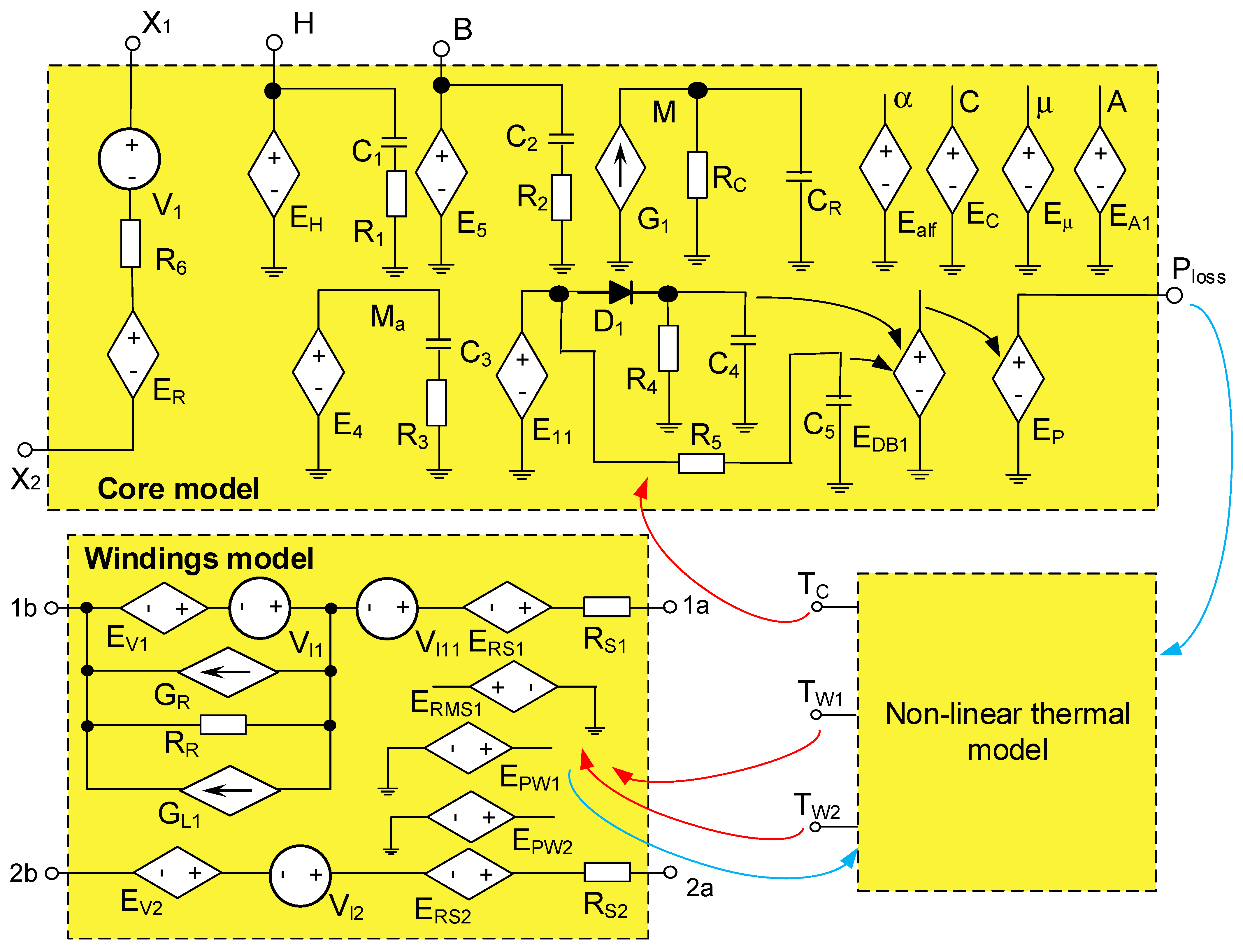
2. Model Form
2.1. Core Model
2.2. Windings Model
2.3. Non-Linear Thermal Model
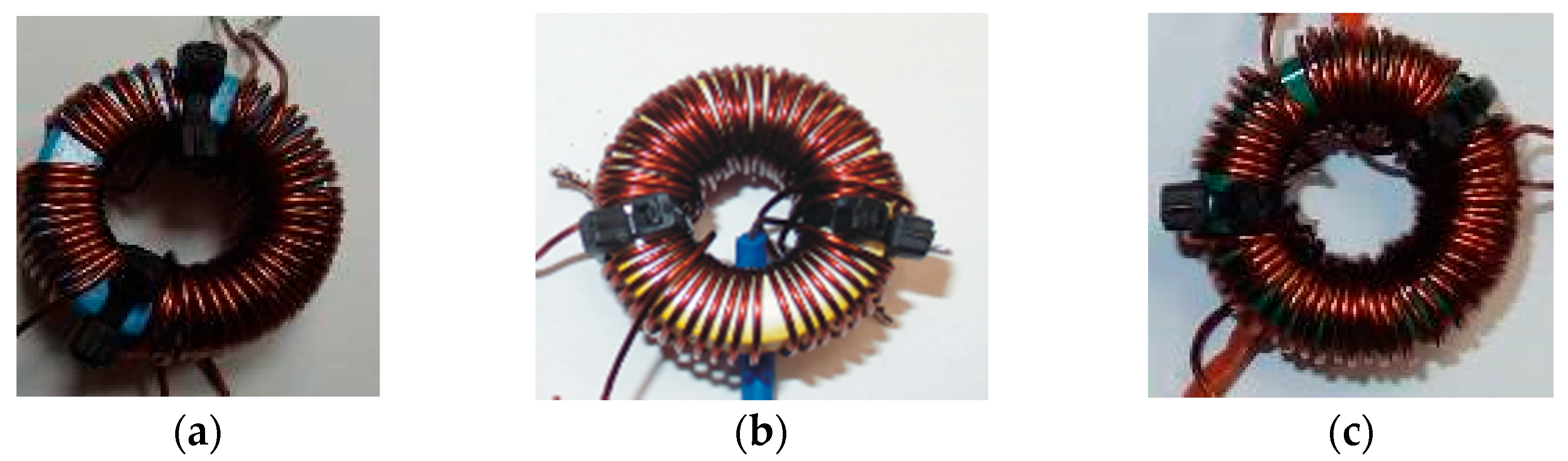
3. Investigated Devices
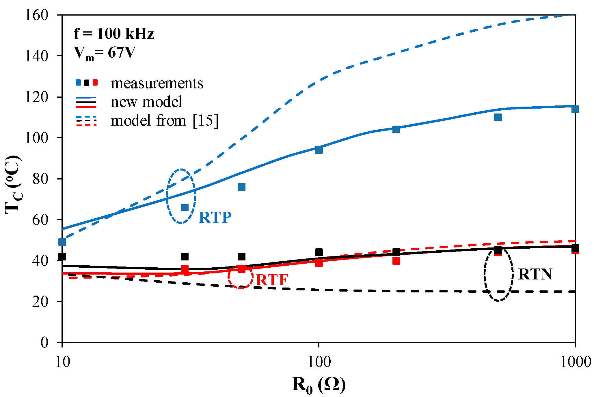
4. Investigations Results
4.1. Ring Transformers
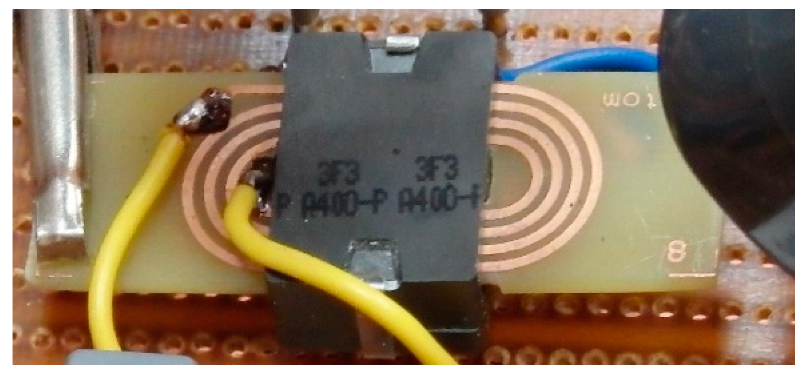
4.2. Planar Transformers
5. Conclusions
Author Contributions
Funding
Institutional Review Board Statement
Informed Consent Statement
Data Availability Statement
Conflicts of Interest
References
- Ericson, R.; Maksimovic, D. Fundamentals of Power Electronics; Kluwer Academic Publishers: Norwell, MA, USA, 2001. [Google Scholar]
- Kazimierczuk, M.K. Pulse-Width Modulated DC-DC Power Converters; John Wiley & Sons: Hoboken, NJ, USA, 2008. [Google Scholar]
- Rashid, M.H. Power Electronic Handbook; Academic Press: Cambridge, MA, USA; Elsevier: Amsterdam, The Netherlands, 2007. [Google Scholar]
- van den Bossche, A.; Valchev, V.C. Inductors and Transformers for Power Electronics; Taylor & Francis Group/CRC Press: Boca Raton, FL, USA, 2005. [Google Scholar]
- Kazimierczuk, M.K. High–Frequency Magnetic Components; John Wiley & Sons: Hoboken, NJ, USA, 2014. [Google Scholar]
- Górecki, K.; Rogalska, M. The compact thermal model of the pulse transformer. Microelectron. J. 2014, 45, 1795–1799. [Google Scholar] [CrossRef]
- Wilson, P.R.; Ross, J.N.; Brown, A.D. Simulation of magnetic component models in electric circuits including dynamic thermal effects. IEEE Trans. Power Electron. 2002, 17, 55–65. [Google Scholar] [CrossRef]
- Tsli, M.A.; Amoiralis, E.I.; Kladas, A.G.; Souflaris, A.T. Power transformer thermal analysis by using an advanced coupled 3D heat transfer and fluid flow FEM model. Int. J. Therm. Sci. 2012, 53, 188–201. [Google Scholar] [CrossRef]
- Górecki, K.; Detka, K.; Górski, K. Compact thermal model of the pulse transformer taking into account nonlinearity of heat transfer. Energies 2020, 13, 2766. [Google Scholar] [CrossRef]
- Basso, C.P. Switch-Mode Power Supply SPICE Cookbook; McGraw-Hill: New York, NY, USA, 2001. [Google Scholar]
- Maksimovic, D.; Stankovic, A.M.; Thottuvelil, V.J.; Verghese, G.C. Modeling and simulation of power electronic converters. Proc. IEEE 2001, 89, 898–912. [Google Scholar] [CrossRef]
- Górecki, P.; Wojciechowski, D. Accurate computation of IGBT junction temperature in PLECS. IEEE Trans. Electron Devices 2020, 67, 2865–2871. [Google Scholar] [CrossRef]
- Górecki, K.; Zarębski, J. The method of a fast electrothermal transient analysis of single-inductance dc-dc converters. IEEE Trans. Power Electron. 2012, 27, 4005–4012. [Google Scholar] [CrossRef]
- Godlewska, M.; Górecki, K.; Górski, K. Modelling the pulse transformer in SPICE. IOP Conf. Series Mater. Sci. Eng. 2016, 104, 012011. [Google Scholar] [CrossRef] [Green Version]
- Górecki, K.; Godlewska, M. Modelling characteristics of the impulse transformer in a wide frequency range. Int. J. Circuit Theory Appl. 2020, 48, 750–761. [Google Scholar] [CrossRef]
- Penabad-Duran, P.; Lopez-Fernandez, X.M.; Turowski, J. 3D non-linear magneto-thermal behavior on transformer covers. Electr. Power Syst. Res. 2015, 121, 333–340. [Google Scholar] [CrossRef]
- Wilamowski, B.; Jager, R.C. Computerized Circuit Analysis Using SPICE Programs; McGraw-Hill: New York, NY, USA, 1997. [Google Scholar]
- Poppe, A.; Farkas, G.; Gaál, L.; Hantos, G.; Hegedüs, J.; Rencz, M. Multi-Domain Modelling of LEDs for Supporting Virtual Prototyping of Luminaires. Energies 2019, 12, 1909. [Google Scholar] [CrossRef] [Green Version]
- Górecki, K.; Zarębski, J.; Górecki, P.; Ptak, P. Compact thermal models of semiconductor devices—A review. Int. J. Electron. Telecommun. 2019, 65, 151–158. [Google Scholar]
- D’Alessandro, V.; Rinaldi, N. A critical review of thermal models for electro-thermal simulation. Solid State Electron. 2002, 46, 487–496. [Google Scholar] [CrossRef]
- Jiles, D.C.; Atherton, D.L. Theory of ferromagnetic hysteresis. J. Magn. Magn. Mater. 1986, 61, 48–60. [Google Scholar] [CrossRef]
- Górecki, K.; Górski, K. Compact electrothermal model of an impulse transformer for SPICE. In Proceedings of the 14th International Conference on Compatibility, Power Electronics and Power Engineering CPE-POWERENG, Setubal, Portugal, 8–10 July 2020; pp. 82–87. [Google Scholar]
- Mawby, P.A.; Igic, P.M.; Towers, M.S. Physically based compact device models for circuit modelling applications. Microelectron. J. 2001, 32, 433–447. [Google Scholar] [CrossRef]
- Maxim, A.; Andreu, D.; Boucher, J. Novel behavioral method of SPICE macromodeling of magnetic components including the temperature and frequency dependencies. In Proceedings of the IEEE Application Power Electronics Conference and Exposition APEC’98, Anaheim, CA, USA, 15–19 February 1998; Volume 1, pp. 393–399. [Google Scholar]
- Górecki, K.; Górski, K. Modelling nonisothermal electrical characteristics of ferrite cores. J. Phys. Conf. Ser. 2018, 1033, 012005. [Google Scholar] [CrossRef]
- Górecki, K.; Rogalska, M.; Zarębski, J.; Detka, K. Modelling characteristics of ferromagnetic cores with the influence of temperature. J. Phys. Conf. Ser. 2014, 494, 012016. [Google Scholar] [CrossRef] [Green Version]
- Barlik, R.J.; Nowak, K.M. Energoelektronika. Elementy Podzespoły, Układy; Oficyna Wydawnicza Politech: Warsaw, Poland, 2014; ISBN 978-83-7814-062-7. [Google Scholar]
- Górecki, K.; Górecki, P. Nonlinear compact thermal model of the IGBT dedicated to SPICE. IEEE Trans. Power Electron. 2020, 35, 13420–13428. [Google Scholar] [CrossRef]
- 3F3 Material Specification. Ferroxcube. 2008. Available online: http://ferroxcube.home.pl/prod/assets/3f3.pdf (accessed on 20 August 2021).
- Iron Powder Toroidal Core for Power Applications. Power Conversion & Line Filter Applications, Micrometels Iron Powder Cores. Available online: https://www.acalbfi.com/nl/Magnetic-components/Cores/Iron-Powder/p/Iron-powder-toroidal-core-for-power-applications/0000000BNV (accessed on 20 August 2021).
- Product Specification for Inductive Components. Available online: https://www.magnetec.de/wp-content/uploads/2018/11/m-070.pdf (accessed on 20 August 2021).
- F-867 Material Characteristics. Available online: http://sklep.remagas.pl/images/W%C5%82a%C5%9Bciwo%C5%9Bci_materia%C5%82u_F-867.pdf (accessed on 20 August 2021).


| Name of Variable | Symbol | SPICE Voltage |
|---|---|---|
| Magnetic force | H | v(H) |
| Magnetic flux density | B | v(B) |
| Magnetization | M | v(M) |
| Power losses in the core | Ploss | v(Ploss) |
| Voltage between the core terminals | v | v(X1,X2) |
| Temperature of the core | TC | V(TC) |
| Temperature of the primary winding | TW1 | V(TW1) |
| Temperature of the secondary winding | TW2 | V(TW2) |
| Results Presented in Figures | Transformer with the Core | |||
|---|---|---|---|---|
| Ring RTN | Ring RTF | Ring RTP | Planar 3F3 | |
| Figure 5, Figure 6, Figure 7 and Figure 8 | 3435.5 s | 2335.5 s | 10,083.5 s | - |
| Figure 9 and Figure 10 | 13,736 s | 3826.8 s | 107,224.8 s | - |
| Figure 11, Figure 12 and Figure 13 | - | - | - | 16,477.7 s |
Publisher’s Note: MDPI stays neutral with regard to jurisdictional claims in published maps and institutional affiliations. |
© 2021 by the authors. Licensee MDPI, Basel, Switzerland. This article is an open access article distributed under the terms and conditions of the Creative Commons Attribution (CC BY) license (https://creativecommons.org/licenses/by/4.0/).
Share and Cite
Górecki, K.; Górski, K. SPICE-Aided Compact Electrothermal Model of Impulse Transformers. Appl. Sci. 2021, 11, 8894. https://doi.org/10.3390/app11198894
Górecki K, Górski K. SPICE-Aided Compact Electrothermal Model of Impulse Transformers. Applied Sciences. 2021; 11(19):8894. https://doi.org/10.3390/app11198894
Chicago/Turabian StyleGórecki, Krzysztof, and Krzysztof Górski. 2021. "SPICE-Aided Compact Electrothermal Model of Impulse Transformers" Applied Sciences 11, no. 19: 8894. https://doi.org/10.3390/app11198894
APA StyleGórecki, K., & Górski, K. (2021). SPICE-Aided Compact Electrothermal Model of Impulse Transformers. Applied Sciences, 11(19), 8894. https://doi.org/10.3390/app11198894