A Two-Stage Hybrid Metaheuristic for a Low-Carbon Vehicle Routing Problem in Hazardous Chemicals Road Transportation

Abstract

Low-carbon economy advances the sustainable development of the transportation of hazardous chemicals. This paper focuses on the multi-trip heterogeneous vehicle routing problem that includes the prioritization of customers and transportation of incompatible cargoes (MTHVRP-PCIC) in which some customers are prioritized for delivery by heterogeneous vehicles and more than one type of cargo is transported. This is an issue because some cargoes are incompatible with each other and therefore cannot be loaded into the same vehicle. MFHVRP-PCIC aims to find a set of routes resulting in minimal costs including fixed cost, travel cost and carbon emission cost. This problem occurs in real-life applications in the hazardous chemicals road transportation industry. This paper contributes to addressing the MTHVRP-PCIC from a problem definition, model, and methodological point of view. We establish a mathematical formulation for this problem. A two-stage hybrid metaheuristic approach (TSHM) is also devised to solve this problem. First, an improved greedy randomized adaptive search procedure is designed to generate initial feasible solutions. Then, a hybrid genetic algorithm including local search strategies, split-feasibility procedure, and simulated annealing is designed to solve this problem. Finally, the proposed approach is applied to solve a real case of hazardous chemical delivery and a benchmark dataset, and the resulting solutions indicate the advantage of our algorithm compared with those solutions obtained from managerial experience and classical algorithms.

1. Introduction

In recent years, the low-carbon concept is widely popularized in society, which uses new technologies and modes to reduce carbon emissions. As a supporting industry, logistics-related enterprises contribute a lot of the total carbon emissions. Subsequently, road transport contributed 92% of total CO₂ emissions for freight transport in China among various modes, and roughly 6% of total domestic CO₂ emissions [1]. Fahimnia et al. [2] presented that increased awareness of environmental issues has resulted in a shift towards creating environmentally sustainable logistics planning and it is key to incorporate environmental concerns in planning and optimization of existing logistics systems. Dekker et al. [3] stated that operations research leads to a more efficient use of resources, which is not only cost-attractive, but also tends to create less emissions of greenhouse gases through the identification of trade-offs between environmental aspects and costs. Hence, low carbon practices should be integrated into logistics operations. Low carbon logistics has attracted increased attention in logistics operations from enterprises and professionals [4,5].

The vehicle routing problem (VRP) is a well-known combination optimization problem in logistics operations and exists in many real-life situations, such as school bus scheduling [6], snow removal and street sweeping [7], waste collection [8], and so on. It aims to identify a set of transport routes to provide efficient service to all customers with minimum cost. It was first proposed by Dantzig and Ramser in 1959 [9] and many kinds of variants of VRP have been developed since [10]. In this paper, we explore a new variant of VRP called the multi-trip heterogeneous vehicle routing problem with prioritized customers and incompatible cargoes (MTHVRP-PCIC) which is inspired by a real application in the hazardous chemicals road transportation industry. The problem differs from the general vehicle routing problem (GVRP) in the following five aspects: (1) the vehicles are heterogeneous; (2) some customers are given priority over others; (3) more than one kind of cargo is transported and some cargo types are incompatible with others, which means they cannot be loaded into the same vehicle; (4) the vehicles can continue to serve customers after returning to the depot within the trip duration; and (5) carbon emission cost is considered.

The study aims to reach a trade-off between cost (including fixed cost and travel cost) and carbon emissions through integrating the low carbon economy into the logistics operations. A route optimization model in terms of the characteristics of road transportation of hazardous chemicals is developed. A two-phase hybrid metaheuristic algorithm is designed to solve the problem. The overall cost and carbon emissions are reduced with the developed model and solution method.

The remainder of this paper is organized as follows. Related literature is presented in Section 2. Section 3 defines and describes the problem and develops the formulation mathematically for optimizing the route plan. This is followed by Section 4 which devises a two-phase hybrid metaheuristic algorithm. Section 5 outlines key data from road transportation practices for hazardous chemicals, which will be used as inputs to test the performance of the model and algorithm. Finally, the conclusion is presented in Section 6.

2. Literature Review

To the best of our knowledge, this is the first time the MTHVRP-PCIC has been the focus of a study despite its many real applications in practice. Related literature is listed as follows: (Section 2.1) low-carbon vehicle routing problem (LCVRP), and (Section 2.2) multi-trip vehicle routing problem (MTVRP). The researchers of the two aspects and their differences within the MTHVRP-PCIC are analyzed as follows:

2.1. Low–Carbon Vehicle Routing Problem

Environmental sustainability is emerging as an important factor affecting business today and it is also one of the critical factors in modern logistics industry [11,12]. Tang et al. [13] studied the issue of cutting emissions by reducing shipment trips and formulated a benchmark model to represent the business-as-usual scenario; the results showed the firm could meet a moderate emission reduction target by reducing shipment trips. Yang et al. [14] focused on the reduction of carbon emissions in the city logistics distribution network and proposed a novel low-carbon tax-constrained city logistics distribution network planning mode; the empirical study shows that the new model can help operators save up to 9.2% of operational costs, reducing carbon dioxide discharge by around 54.5%. Furthermore, Wang et al. [15] studied the green distribution network with electric vehicles and fuel vehicles in which operators achieve a win-win scenario including a reduction in carbon emissions and distribution costs. Xiao and Konak [16] proposed a CO₂ emission optimization approach based on time-varying traffic congestion with promising results to help road-based delivery enterprises and individual drivers make better plans with lower carbon emissions and reduced fuel consumption. Soysal et al. [17] focused on the impact of explicit fuel consumption, variable vehicle speed on the carbon emissions, and the results showed that considering these factors can reduce significant transportation costs and carbon emissions. Li et al. [18] studied the green vehicle routing problem (GVRP) considering carbon emissions and proposed an improved ant colony optimization algorithm using an innovative approach which updated ant pheromones to solve this problem. More studies on the GVRP can be seen in [5,19,20,21].

The differences between the MTHVRP-PCIC and the GVRP can be concluded as follows: most researchers considered carbon emissions in terms of conventional vehicle routing problems, and few researches focused on the characteristics of customers and cargo types in the GVRP. The severe impact of hazardous chemicals, along with significant casualties and environmental pollution, necessitates further improvements in transportation planning.

2.2. Multi-Trip Vehicle Routing Problem (MTVRP)

The MTVRP is a new variant of VRP that is attracting increasing attention, in which vehicles can be used more than once during the planning period. Brandao and Mercer [22] first proposed the multi-trip vehicle routing problem and designed a tabu search algorithm addressing this issue. Furthermore, Nguyen et al. [23] focused on the time-dependent multi-zone multi-trip vehicle routing problem with time windows (MZMT-VRPTW) in which customers are clustered in zones, each of which has a supply point; vehicles can serve different zones, but must visit the supply point before visiting the corresponding zone. Other variants of the MTVRP include: MTVRP with pickup and delivery of customers to the airport [24], MTVRP with limited duration [25], MTVRP with multi-commodity [26], MTVRP with time windows and release dates [27], MTVRP with separate pickup and delivery and time windows for customers and facilities [28], and two-echelon MTVRP with dynamic satellites [29].

The differences between the MTHVRP-PCIC and the MTVRP can be described as follows: (1) some of the cargoes in the MTHVRP-PCIC are incompatible and cannot be transported in the same vehicle while cargoes in the MTVRP can and (2) customers have different delivery priorities in the MTHVRP-PCIC while customers are equal in the MTVRP.

In conclusion, as a result of the above literature review, there are no existing methods or models addressing the MTHVRP-PCIC. In addition, as an extension of basic VRP which is a well-known NP-hard problem, the MTHVRP-PCIC is also a NP-hard problem which means that a small instance of the MTHVRP-PCIC could create great complexity to solve. Therefore, we designed a two-stage hybrid metaheuristic approach (TSHM) to solve this problem. Experiments were made to validate the effectiveness of our proposed algorithm. The main contribution of this study is as follows:

• Low-carbon economy advances the transportation of hazardous chemicals in the road transportation industry.
• Multi-trip, heterogeneous vehicles, prioritized customers, and incompatible cargoes are considered.
• An innovative two-phase heuristics algorithm is devised which balances the load rate and minimizes the transportation cost.
• The proposed solution approach is applied to a large-scale real case study.

3. Problem Description and Formulation

3.1. Problem Description and Characteristics

The multi-trip heterogeneous vehicle routing problem with prioritized customer and incompatible cargoes (MTHVRP-PCIC) is formally defined as follows. Let $G=\left(N,A\right)$ with $N=\left(0,1,\cdots n\right)$ be a complete directed graph in which node 0 represents the depot from where special vehicles start and the remaining nodes correspond to the locations of customers (such as factories or research institutes). Each arc $\left(i,j\right)\in A$ has an associated travel distance $d_{ij}$ and travel cost $c_{ijv}$ for special vehicles v per kilometer. The locations of customers is represented by $C$. The delivery for a customer $i\in C$ is characterized by a demand quantity $d_i$.

In the real world, a customer may require different kinds of goods that are not permitted to be loaded into the same vehicle (such as inflammable gas and combustion-supporting chemical reagents), which results in more than one delivery for such customers. To model the problem succinctly, we divided customer $i\in C$ with demand quantity $d_i^a$ for cargo $a$ and $d_i^b$ for cargo $b$ into two customers $i$ with demand quantity $d_i=d_i^a$ and customer $n+1$ with demand quantity $d_{n+1}=d_i^b$, and then $n\to n+1$. It should be noted that these two customers are in the same location. The above process is repeated for the remaining customers with different kinds of cargo that are permitted to be loaded into the same vehicle. Therefore, each customer will then be visited only once per vehicle.

The MFHVRP-PCEC developed in this paper has the following characteristics:

• The vehicles are heterogeneous;
• Some of customers have priority over others;
• More than one kind of cargo is transported and some cargoes are not permitted to be loaded into the same vehicle;
• Each vehicle starts and ends at the depot;
• Each vehicle cannot exceed the capacity limit;
• Each customer is visited only once;
• Each vehicle can continue to serve customers again after returning to the depot within the transport planning period.

3.2. Formulation

Let $x_{ijv}^f$ be a binary variable indicating whether arc $\left(i,j\right)\in A$ is traveled or not by vehicle v at f-th trip, where $f\in F$ represents the transportation trip. We define $x^f\left(A\prime \right)={\displaystyle {\sum }_{v\in V}{\displaystyle {\sum }_{\left(i,j\right)\in A\prime }{x}_{ijv}^f}}$ for $A\prime \subseteq A$ and we use ${\alpha }^{-}\left(i\right)$ and ${\alpha }^{+}\left(i\right)$ to denote the sets of incoming and outgoing arcs of node $i$, respectively.

3.2.1. Cost Analysis

This study not only aims to minimize the total travel distance, but also the costs caused by carbon emissions. The objective is to reach a trade-off among the number of vehicles used and travel costs and carbon emissions. The comprehensive costs include fixed cost, travel cost, and carbon emission cost produced by the special vehicles that deliver hazardous chemicals.

(a)

Fixed cost

Fixed cost is dependent on the number of special vehicles used including the depreciation of special vehicles and the drivers’ salaries. Considering f transportation frequencies for special vehicles $v\in V$, the fixed cost of special vehicles is computed as:

$$C_1={\displaystyle \sum _{f\in F}{\displaystyle \sum _{v\in V}{\displaystyle \sum _{j\in N\backslash \left\{0\right\}}{c}_v{x}_{0jv}^f}}}$$

(1)

where $c_v$ is the fixed cost of special vehicles v.

(b)

Travel cost

Travel cost is dependent on travel distances during the delivery process. The travel cost is computed as follows:

$$C_2={\displaystyle \sum _{v\in V}{\displaystyle \sum _{f\in F}{\displaystyle \sum _{\left(i,j\right)\in A}{w}_v{d}_{ij}{x}_{ijv}^f}}}$$

(2)

where $w_v$ is the variable cost of special vehicles v.

(c)

Carbon emission cost

The carbon emission cost is similar to the cost of CO2 emissions during the delivery [30]. This includes carbon emissions produced by consumption of fuel which is related to the load and travel distance of special vehicles. The carbon emission cost is computed as follows:

$$C_3=p{\displaystyle \sum _{v\in V}{\displaystyle \sum _{f\in F}{\displaystyle \sum _{\left(i,j\right)\in A}eE\left(q_{ij}\right)d_{ij}{x}_{ijv}^f}}}$$

(3)

where $e$ is the emission factor of CO₂ and p is the unit carbon tax. $E\left(q_{ij}\right)$ is the relationship between unit distance fuel consumption and load, which can be computed as follows [31]:

$$E\left(q_{ij}\right)=\frac{{\epsilon }_{mv}-{\epsilon }_{0v}}{Q_v}{q}_{ijv}^f+{\epsilon }_{0v}$$

(4)

where ${\epsilon }_{mv}$ is the unit distance fuel consumption with a full load of special vehicles v. ${\epsilon }_{0v}$ is the unit distance fuel consumption with an empty load of special vehicles v. $Q_v$ is the maximum load of special vehicles v. $q_{ijv}^f$ is the freight quantity delivered by special vehicles v from node i to j at f-th trip.

3.2.2. Establishment of the Model

The proposed MFHVRP-PCEC is formulated as shown below:

$$Min{C}_1+C_2+C_3$$

(5)

$$x^f\left({\alpha }^{-}\left(i\right)\right)-x^f\left({\alpha }^{+}\left(i\right)\right)=0,\forall i\in C,f\in F$$

(6)

$${\displaystyle \sum _{f\in F}{x}^f\left({\alpha }^{-}\left(i\right)\right)}=1,\forall i\in C$$

(7)

$$x^f\left({\alpha }^{+}\left(0\right)\right)\le \left|V\right|,\forall f\in F$$

(8)

$$y_{jv}^f\ge y_{iv}^f+d_j-Q_v\left(1-x_{ijv}^f\right),\forall f\in F,v\in V$$

(9)

$$0\le y_{iv}^f\le Q_v-d_i,\forall i\in C,f\in F,v\in V$$

(10)

$$x_{ijv}^f\in \left\{0,1\right\},\forall i,j\in C,f\in F,v\in V$$

(11)

where $y_{iv}^f$ is the cargo quantity remaining after service at customer i by vehicle v at its f-th trip. The objective is to minimize the total transportation cost of all vehicles in Constraint (5). Constraint (6) captures the vehicle flow conservation at each customer. Each customer is visited only once in Constraint (7). The number of vehicle departures from the depot is limit at most $\left|V\right|$ by Constraint (8). Constraints (9) and (10) ensure that the required quantities are transported to the customers and each route does not exceed the vehicle capacity. The decision variables are captured by Constraint (11).

4. Solution Method

The goal of the solution method is to obtain an approximate optimum solution for this issue. We designed a two-stage hybrid metaheuristic approach (TSHM) organized as follows: in the first stage we applied an improved greedy randomized adaptive search procedure (I-GRASP) to generate M initial feasible solution, then order them by non-decreasing cost and the first $M*$ is selected as the initial population. The second stage is to improve the initial population by means of a hybrid genetic algorithm (HGA). In each iteration, the crossover and mutation operators are applied on the population to enhance search intensification and diversification, while a local search strategy is used to reach local optimum and a split-feasibility procedure (SFP) to make improved solutions feasible, and a simulated annealing (SA) is used to accept the improved solution or not. The procedure of this algorithm is shown in Figure 1. The details of this algorithm are presented in the following sub-section.

4.1. I-GRASP

To tackle the multiple attributes (such as multi-trip, priority customers, and incompatible cargo) of this issue, we designed an improved greedy randomized adaptive search procedure (I-GRASP) to generate high-quality initial feasible solutions. The procedures are as follows:

• For not-yet-visited customers, insert deliveries by each location on all the trips on all the routes (including the empty trip routes) respecting capacity, customer priority, and cargo attributes, then evaluate the cost change induced by the insertion operation.
• Rank the insertion by non-decreasing cost and choose randomly one from the first K most profitable ones.
• Continue the above steps till all customers have been visited.

In our experiments, we generate M = 100 initial solutions and sort them by non-decreasing cost and select first M* = 50 ones as the input of the second stage metaheuristic; Algorithm 1 outlines the I-GRASP in pseudo-code.

Algorithm 1 I-GRASP

Input: Solution size M. Customer data.

Output: the first M* feasible solution S.

Pool$\leftarrow \varnothing$

For count$\leftarrow$1 to M do

Unvisited customer set$\leftarrow$$C$

Initial Solution IS$\leftarrow \varnothing$

While Unvisited customer set $\ne \varnothing$ do

If IS does not include an empty route or empty trip for each route then

Add an empty route in IS or empty trip in these routes without an empty trip

End

Insert not visited customers into each location of each trip on all routes (satisfy all constraints in the model)

Calculate cost changes for all insertions, then sort them and store in Candidate List

Select a candidate insertion randomly from first K candidates and implement it

Unvisited customer set$\leftarrow$ Unvisited customer set$\backslash c$

End while

$Pool\stackrel{append}{\leftarrow }IS$

End for

Sort all initial feasible solutions by non-decreasing cost, then

Add first M* ones into S

Return S

4.2. Hybrid Genetic Algorithm

4.2.1. Algorithm Overview

The proposed HGA for the MTHVRP-PCIC consists of the traditional genetic operators (crossover, mutation and selection) in addition to the new strategies: (1) local search (LS), (2) split-feasibility procedure (SFP), and (3) simulated annealing (SA). The LS is responsible for exploring the local optimal neighborhood of this current solution. The SFP not only makes the improved solutions feasible for the constraints in the model after crossover and mutation, but also enhances search intensification and diversification. The SA avoids the algorithm falling into local optimum too early. Algorithm 2 presents the pseudo-code.

Algorithm 2 HGA

Input: initial population M* and other parameters;

Output: the best solution found BestSol;

while stop criteria not reached do

Apply crossover operator to generate offspring individual $s\prime$

Apply mutation operator to generate offspring individuals $s\prime$

Apply local search strategy to generate improved neighborhood solution $s\prime$

Apply split-feasibility procedure to make new solution feasible

for each new individual generated at each step above do

if $c\left(s\prime \right)\le c\left(s\right)$ then

$s:=s\prime$

else

if $c\left(s\prime \right)>c\left(s\right)$ then

$s:=s\prime$

else

$s:=s\prime$ with probability p defined in Section 4.2.5

end for

end while

Return BestSol

4.2.2. Genetic Operators

In this section we designed a 2-point crossover operation and multi-point mutation operation to improve the current population and explore solution space. The 2-point crossover operation is described in detail as follows:

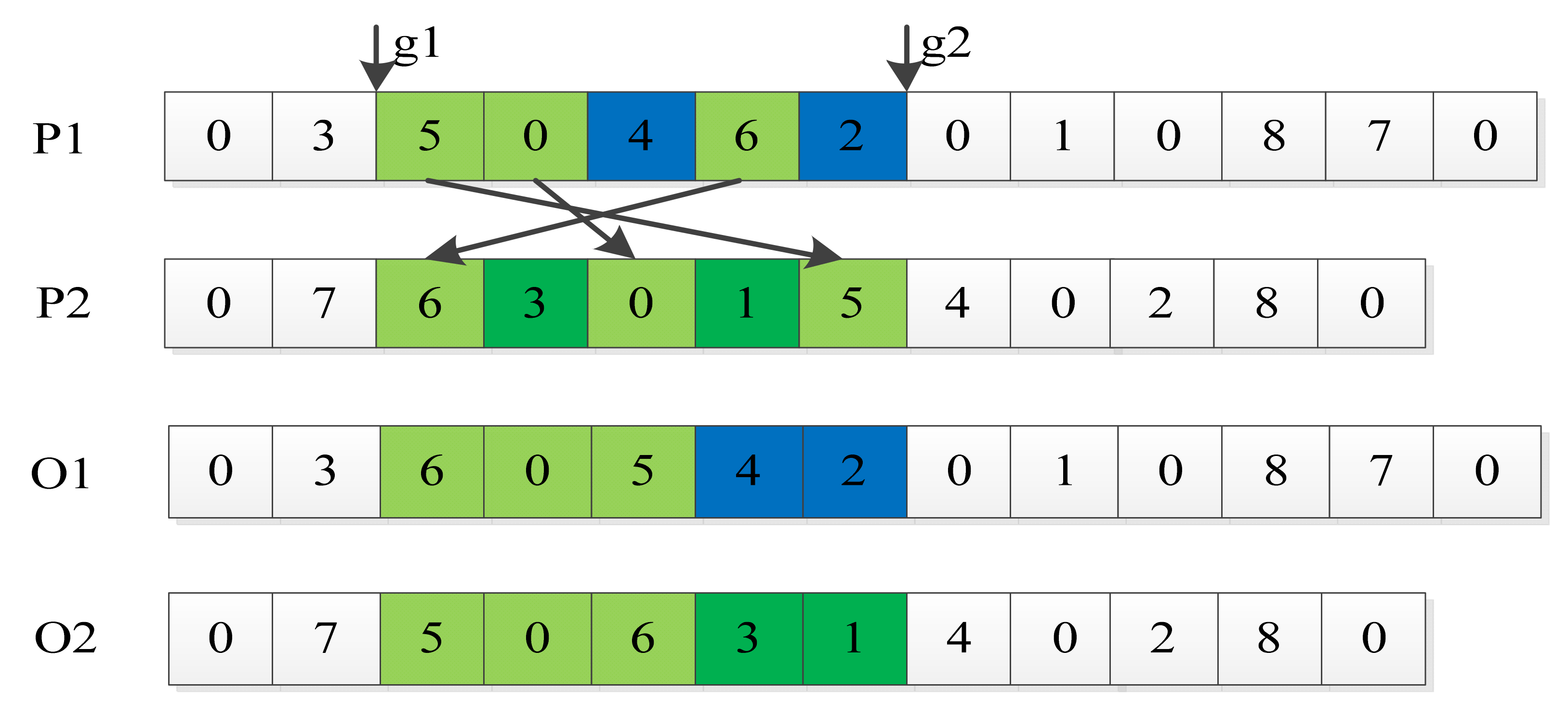
Step 1: 

select randomly two individuals (P1 and P2) with crossover probability $p_c$;

Step 2: 

select randomly two crossover genes (g1 and g2) ranging from 0 to $n_{\min }$, and $n_{\min }$ is the number of customers with less customers between the two individuals;

Step 3: 

add the same genes into set S0 (5, 0, and 6) sequentially between g1 and g2 for individual P1, and add the same genes into set S1 (6, 0, and 5) sequentially between g1 and g2 for individual P2;

Step 4: 

for individual P1, add the genes into set S2 (4 and 2) which is different with P2 between g1 and g2, and for individual P2, add the genes into set S3 (3 and 1) which is different with P1 between g1 and g2;

Step 5: 

reinsert S0 and S3 into P2 sequentially between g1 and g2, and then get an offspring individual O2; and reinsert S1 and S2 into P1 between g1 and g2, and then get an offspring individual O1.

An example is given to illustrate this operation in Figure 2.

In the mutation operation, we designed multi-point mutation operations to generate new offspring individuals. The procedure is as follows:

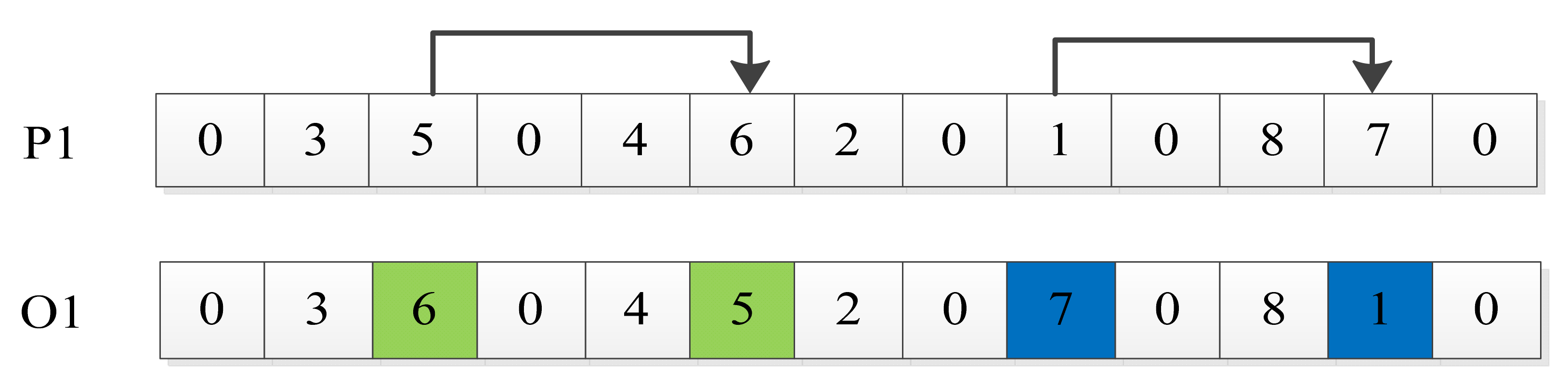
Step 1: 

select an individual randomly with mutation probability $p_m$;

Step 2: 

select a gene (such as g1 = 6) randomly on the individual and revise it into another gene (such as g2 = 5) randomly;

Step 3: 

check if there is the same gene as g2 on other locations, if yes, then revise the gene into g1 = 6; and

Step 4: 

repeat step 2–step 3 m times;

An example is given to illustrate this operation in Figure 3.

4.2.3. Local Search Strategy

In this section, we applied a local search, which is a classical optimization algorithm, to improve the solutions. During the procedure, neighborhood strategies are defined to generate new solutions by means of destroying old solutions. Hence, designing effective neighborhood strategies is important to generate better solutions. Six neighborhood strategies are used as follows [32] (see Figure 4):

• Intra-route swap: for any route, select randomly two customers and exchange them;
• Intra-route relocate: for any route, remove randomly a customer and reinsert it into another location on the same route;
• Intra-route 2-opt: for any route, select randomly two lists of sequential customers and reverse these customers between them, and exchange the two lists of sequential customers;
• Inter-route swap: select randomly one customer from two routes respectively, and exchange them;
• Intra-route relocate: remove randomly a customer on a route and reinsert it into another route;
• Inter-route 2-opt: select sequential customers on a route randomly; do the same for another route and exchange them.

4.2.4. Split-Feasibility Procedure (SFP)

In genetic operations and local search procedures, some infeasible solutions may be generated. It is time-consuming and inefficient to simply delete these infeasible solutions. In this section, we designed a split-feasibility procedure (SFP) to make infeasible solutions feasible. The procedures are as follows:

Step 1: 

check if the chromosome is feasible, if yes, turn to step 4, or turn to step 2;

Step 2: 

regard the genes of this chromosome as an unvisited customer set S, a random-selection and greedy-insertion heuristic is designed to generate new feasible chromosomes as follows:

Step 2.1: 

select one of the remaining customers from S randomly, reinsert it into a new chromosome;

Step 2.2: 

evaluate the cost change induced by the above insertion operation at each point of the chromosome;

Step 2.3: 

rank the insertion operations by nondecreasing cost and keep the most profitable one.

Step 2.4: 

repeat Steps 2.1–2.3 until all customers are reinserted into the chromosomes.

Step 3: 

generate G new chromosomes, and select the lowest cost one as the output.

Step 4: 

Output the obtained chromosome.

4.2.5. Simulated Annealing (SA)

At each iteration, simulated annealing (SA) is used to accept new individuals or not, which promotes search intensification and diversification. Let $s$ be the current individual, $s\prime$ be the new individual, and $c\left(s\right)$,$c\left(s\prime \right)$ be the corresponding objective values. If $c\left(s\prime \right)$ is better than $c\left(s\right)$, we accept the new individual $s\prime$, or we accept the individual $s$ with probability p:

$$p=\min \left\{1,e^{\left(c\left(s\prime \right)-c\left(s\right)\right)/T}\right\}$$

(12)

where $T\ge 0$ is the “temperature” which starts at $T_0$ and reduces each iteration by the expression $T:=0.99T$. $T_0$ is a defined probability value, such as 0.5. The SA procedure is seen in Algorithm 2.

5. Case Study and Analysis

5.1. Data

This section presents the data of customers seen in

Table 1. Data of customer information.

ID	X	Y	Priority	Demand	Types	ID	X	Y	Priority	Demand	Types
0	118.64611	31.94249	0	0	0	24	118.84352	31.86329	0	33	A
1	118.72178	32.20923	1	3	A	25	118.98820	32.10691	0	20	A
2	119.37719	32.17857	0	10	B	26	118.96864	31.37930	0	32	C
3	119.02719	32.14194	0	32	A	27	118.96865	32.37930	0	2	A
4	118.37410	32.34485	1	16	A	28	118.83423	32.26079	0	30	A
5	118.35853	32.33745	0	10	A	29	118.39192	32.35888	0	64	A
6	119.83227	32.07926	0	1	A	30	118.61083	32.23142	0	19	A
7	119.40095	32.18148	0	54	B	31	118.56196	31.84031	0	45	A
8	119.72228	32.07920	0	54	A	32	118.56196	31.84031	0	32	C
9	118.98790	32.10089	0	32	A	33	118.70426	31.90448	1	15	C
10	118.59852	31.83661	1	10	A	34	118.76532	31.96886	0	2	C
11	118.63642	31.93083	0	12	A	35	118.76532	31.96886	0	3	C
12	118.78055	31.87620	0	16	C	36	118.38382	32.31247	0	45	A
13	118.85628	32.04281	0	8	B	37	118.65598	31.94535	0	32	C
14	118.85628	32.04281	0	4	A	38	118.65598	31.94535	0	16	A
15	119.18360	32.20393	0	5	A	39	118.56172	31.84080	0	15	C
16	118.54957	31.97212	0	10	C	40	118.56172	31.84080	0	25	A
17	118.54957	31.97212	0	10	A	41	118.68243	32.18886	0	4	B
18	118.68316	31.93047	0	20	C	42	119.59338	32.02327	0	15	A
19	118.60298	31.85022	1	22	A	43	118.48638	31.57159	0	32	A
20	118.61282	32.01586	0	16	C	44	118.56265	31.81674	0	32	C
21	119.37209	32.17886	0	18	A	45	118.56265	31.81674	0	16	A
22	119.70852	32.11134	0	20	A	46	118.56196	31.84031	0	4	B
23	118.55725	31.96583	1	10	B	47	118.39209	32.31064	0	16	A

where ID means the identifier number of customers (0 stands for the depot), and X and Y stand for the longitude coordinates and latitude coordinates, respectively. Priority represents the priority of customers (1 means that the customer has to be delivered to first on the tour, customers with priority 0 are delivered to any time). Demand means the demand quantity, and types represents the good property (3 types in total, and B and C are incompatible and cannot be loaded into the same vehicle; others can be combined in the same vehicle). In addition, two kinds of vehicles are used: one with capacity 120 and the other with capacity 176.

5.2. Results

5.2.1. Simulation Examples

The experiment is implemented in JAVA on an Intel Xeon i5-3337U 1.8GHz computer. The effectiveness of the two-stage hybrid metaheuristic approach (TSHM) is verified by solving a practical problem. In this section, a hazardous chemicals road transportation enterprise was chosen as the example. The distribution center has a geographic coordinate of 118.64611 and 31.94249. Other customer information is shown in Table 1. Two kinds of special vehicles were used with capacity of 120 and 176 units, respectively. The former one consists of two vehicles and the latter one consists of three vehicles.

The other parameters of the model are as follows: the fixed costs of two kinds of special vehicles are 70 yuan and 180 yuan; the variable costs are 5 yuan/km and 3 yuan/km; the unit carbon tax is 2 yuan/kg [30]; the emission factor is 2.61 Kg/L [33]; and the unit distance fuel consumption is 0.255L/km with a full load and 0.165L/km with an empty load.

The manmade schedule (MM), basic genetic algorithm (GA), local search strategy (LS), and TSHM are applied to solve the example; the latter three are run 20 times. The results obtained are shown in

Table 2. Results obtained by manmade schedule (MM), GA, TSHM, and LS.

Algorithm	Approximate Optimal Value (yuan)	Average Value (yuan)	Standard Deviation
MM	8550.61	8550.61	0.00
GA	5070.58	5336.54	236.45
TSHM	4199.21	4262.32	42.63
LS	4891.25	5019.92	110.39

, which reports the approximate optimal and average values. Our proposed method obtained the best solution with approximate optimal value and average value (4199.21 and 4282.32 yuan, respectively) which is lower than the other three solutions (5070.58 and 5336.54 yuan for GA, 4891.25 and 5019.92 yuan for LS, and 8550.61 yuan for MM) indicating that the TSHM outperforms the other three methods. The standard deviation obtained by TSHM is also smaller than that obtained by GA and LS, which indicates that TSHM is more stable than GA and LS in terms of stability.

Table 3. Vehicle routes obtained by three methods.

Solution Method	Scheduling Scheme
Manmade schedule	Schedule for vehicles with capacity 120
	Vehicle No.1
	[4, 7] and [8]
	Vehicle No.2
	[1, 29, 21, 22, 42],
	Schedule for vehicles with capacity 176
	Vehicle No.1
	[33, 12, 24, 35, 34, 20, 16, 11, 18, 38, 37] and [23, 17, 47, 36, 46, 40, 31, 45]
	Vehicle No.2
	[19, 6, 26, 43, 44, 32, 39, 5] and [10, 30, 41, 28, 27, 15, 2, 9, 3, 25, 14, 13]
GA	Schedule for vehicles with capacity 120
	Vehicle No.1
	[20, 34, 35, 18, 38, 37] and [1, 30, 28, 13, 14]
	Vehicle No.2
	[19, 45, 44, 40, 11]
	Schedule for vehicles with capacity 176
	Vehicle No.1
	[4, 29, 5, 36, 47, 17, 16] and [23, 41, 27, 22, 6, 8, 9, 46, 31]
	Vehicle No.2
	[33, 12, 24, 26, 43, 32, 39] and [10, 42, 7, 2, 21, 15, 3, 25]
TSHM	Schedule for vehicles with capacity 120
	Vehicle No.1
	[37, 38] and [19, 31, 46, 40, 11]
	Vehicle No.2
	[10, 39, 32, 16, 17, 20]
	Schedule for vehicles with capacity 176
	Vehicle No.1
	[23, 14, 13, 9, 25, 3, 15, 7, 2] and [4, 29, 5, 36, 47, 30, 41]
	Vehicle No.2
	[33, 12, 24, 26, 43, 45, 44] and [1, 28, 27, 21, 22, 6, 8, 42, 35, 34, 18]

shows the approximate optimal routes (only for MM, GA, and TSHM). It is observed that TSHM outperforms the GA in vehicle routing planning. The former not only avoids unnecessary return trips under the condition of meeting customer needs, but also reduces travel cost and carbon emission cost due to a shorter travel distance and profitable delivery visit sequence.

We also solved the model using CPLEX 12.5 and obtained an optimal solution with a cost of 4134.67, consisting of a constant cost of 1080, a travel cost of 2373.3, and a carbon emission cost of 681.37 with a computational time of 29.76 s. The results show that three special vehicles with a capacity of 176 are used, and none with a capacity of 120 are used.

The cost of our solution obtained using our proposed algorithm is 4199.21, and the gap is only 1.5%; however, our algorithm only spent about 1.92 s in solving this problem, which shows the effectiveness of our proposed algorithm.

5.2.2. Impact of Prioritized Customers and Incompatible Cargoes

In order to evaluate the impact of prioritized customers and incompatible cargoes on the system cost, we treated the customers equally, and allowed for all types of cargo to be loaded into the same vehicle. We ran our algorithm 20 times and selected the solution with the lowest cost (see

Table 4. Vehicle routes without prioritized customers and incompatible cargoes.

Without prioritized customers and incompatible cargoes	Scheduling scheme
	Schedule for vehicles with capacity 120
	No
	Schedule for vehicles with capacity 176
	Vehicle No.1
	[45, 44, 46, 31, 32, 40, 39] and [37, 38, 23, 16, 17]
	Vehicle No.2
	[34, 21, 2, 7, 22, 6, 8, 42] and [18, 35, 14, 13, 9, 25, 3, 15, 27, 28, 1, 20]
	Vehicle No.3
	[41, 30, 29, 4, 5, 36, 47] and [11, 19, 10, 43, 26, 24, 12, 33]

). The optimal value was 3882.53 yuan, which is lower than that obtained when considering prioritized customers and incompatible cargoes. This is due to return trips required to serve prioritized customers; in addition, for incompatible cargoes, vehicles have to travel farther and more vehicles are required, which gives enterprises a reason to raise service prices for these customers.

5.3. Performance Analysis of Algorithm

5.3.1. Stability Analysis

To test the stability of TSHM, we ran the instance 100 times with different initial solutions. Overall, the TSHM performed stably in this instance (see Figure 5). Figure 5 shows the relation between the cost of initial (X-axis) and final solutions (Y-axis). We found that the costs of most final solutions are clustered within an interval [4200, 4300], which validates the stability of final solutions obtained by TSHM.

5.3.2. Efficiency Analysis

In this section, we tested the performance of our proposed algorithm, taking three classical datasets designed by Solomon (R101, C101, and RC101) and each with 25 and 100 customers, respectively. Among them, the customer locations of R101 examples were generated randomly, while that of C101 were relatively concentrated, and that of RC101 were uniform. Without loss of generality, about 10% of customers were within priority one generated randomly. The types of products for customers were also generated randomly. The basic GA and the TSHM were applied to solve the benchmarks 10 times, the best results obtained by GA and TSHM are shown in

Table 5. Results obtained by GA and TSHM.

Instance	GA	TSHM	GAP (%)
R101_25_R	2298.21	2256.29	1.82%
R101_100_R	8965.31	7020.73	21.69%
C101_25_R	1845.35	1801.38	2.38%
C101_100_R	7968.58	6362.1	20.16%
RC101_25_R	2754.25	2438.56	11.46%
RC101_100_R	13234.74	9000.26	32.00%
Mean	6177.74	4813.22	22.09%

.

Table 5 shows that the approximate optimal values of the six examples obtained by TSHM were smaller than those of GA. Specifically, the average approximate optimal value for the six examples was less than 22.09% (4813.22 vs. 6177.74). The results demonstrate that the TSHM algorithm was superior to the basic GA.

In addition, we also solved the problem with 25, 50, and 100 nodes using CPLEX 12.5. The computational time was 8.32 seconds and 31.23 seconds for 25 and 50 customers, respectively. However, when there were 100 customers, the CPLEX 12.5 could not solve the problem to obtain the optimal solution within 3600 s. The computational time was within several seconds when using our proposed algorithm to obtain approximately optimal solutions.

6. Conclusions

The low-carbon demand has grown with the development of environment-friendly society and improved quality of living. Moreover, low-carbon economy has also become an increasingly attractive hotspot research field in logistics transportation. This study focused on the multi-trip heterogeneous vehicle routing problem with prioritized customers and incompatible cargoes in the delivery of hazardous chemicals in terms of achieving low-carbon and low-cost economy. We provided a comprehensive consideration of fixed cost, delivery cost, and carbon emission cost.

This study built a mathematical formulation for the delivery of hazardous chemicals considering multiple attributes, which is a further extension of the existing vehicle routing optimization formulation under low-carbon conditions. A mixed integer programming model was established. The genetic algorithm, local search strategy, split-feasibility procedure, and simulated annealing were integrated to avoid the disadvantage of single algorithm and explore more solution space. Our proposed algorithm was verified to outperform the basic genetic algorithm in terms of optimization ability and stability using realistic examples and Solomon benchmark datasets. Our study not only demonstrated the value of operational research for the hazardous chemicals road transportation industry, but also provided a theoretical basis. Our proposed solution method showed high performance compared with the existing schedule and basic genetic algorithm.

Transportation firms should implement a differentiated pricing strategy for different types of customers. Compared with the regular vehicle routing problem considering carbon emission, this paper also focused on the priority of delivery service and good attributes, which not only increases the complexity of the problem, but also increases the delivery cost. Furthermore, firms should investigate customer information before optimizing vehicle routing, and then make decisions based on number of vehicles and which kinds of vehicle are most suitable, or the solution obtained may not be the optimal one according to given vehicles.

Low-carbon logistics transportation is a complex system and an increasingly attractive issue. Most of the existing literature focuses on the regular vehicle routing problem considering carbon emissions and low-costs in terms of building models and algorithm design. Future studies might focus on the optimization of parameter configuration and pricing of transportation service over different kinds of customers.

References

- Piecyk, M.I.; McKinnon, A.C. Forecasting the carbon footprint of road freight transport in 2020. Int. J. Prod. Econ. 2010, 128, 31–42. [Google Scholar] [CrossRef]
- Fahimnia, B.; Reisi, M.; Paksoy, T.; Özceylan, E. The implications of carbon pricing in Australia: An industrial logistics planning case study. Transp. Res. Part. D Transp. Environ. 2013, 18, 78–85. [Google Scholar] [CrossRef]
- Dekker, R.; Bloemhof, J.; Mallidis, I. Operations Research for green logistics An overview of aspects, issues, contributions and challenges. Eur. J. Oper. Res. 2012, 219, 671–679. [Google Scholar] [CrossRef] [Green Version]
- He, Y.; Wang, X.; Zhou, F.; Lin, Y. Dynamic vehicle routing problem considering simultaneous dual services in the last mile delivery. Kybernetes 2019, 49, 1267–1284. [Google Scholar] [CrossRef]
- He, Y.; Zhou, F.; Qi, M.; Wang, X. Joint distribution: Service paradigm, key technologies and its application in the context of Chinese express industry. Int. J. Logist. Res. Appl. 2020, 23, 211–227. [Google Scholar] [CrossRef]
- Kima, B.I.; Park, J. A school bus scheduling problem. Eur. J. Oper. Res. 2012, 218, 577–585. [Google Scholar] [CrossRef]
- Schrage, L. Formulation and structure of more complex/realistic routing and scheduling problems. Networks 1981, 11, 229–232. [Google Scholar] [CrossRef]
- Benjamin, A.; Beasley, J. Metaheuristics for the waste collection vehicle routing problem with time windows, driver rest period and multiple disposal facilities. Comput. Oper. Res. 2010, 37, 2270–2280. [Google Scholar] [CrossRef] [Green Version]
- Dantzig, G.B.; Ramser, J.H. The Truck Dispatching Problem. Manag. Sci. 1959, 6, 80–91. [Google Scholar] [CrossRef]
- Braekers, K.; Ramaekers, K.; Van Nieuwenhuyse, I. The vehicle routing problem: State of the art classification and re-view. Comput. Ind. Eng. 2016, 99, 300–313. [Google Scholar] [CrossRef]
- Ramanathan, U.; Bentley, Y.; Pang, G. The role of collaboration in the UK green supply chains: An exploratory study of the perspectives of suppliers, logistics and retailers. J. Clean. Prod. 2014, 70, 231–241. [Google Scholar] [CrossRef] [Green Version]
- Zhou, F.; He, Y.; Zhou, L. Last Mile Delivery with Stochastic Travel Times Considering Dual Services. IEEE Access 2019, 7, 159013–159021. [Google Scholar] [CrossRef]
- Tang, S.; Wang, W.; Yan, H.; Hao, G. Low carbon logistics: Reducing shipment frequency to cut carbon emissions. Int. J. Prod. Econ. 2015, 164, 339–350. [Google Scholar] [CrossRef]
- Yang, J.; Guo, J.; Ma, S. Low-carbon city logistics distribution network design with resource deployment. J. Clean. Prod. 2016, 119, 223–228. [Google Scholar] [CrossRef]
- Wang, J.; Lim, M.K.; Tseng, M.-L.; Yang, Y. Promoting low carbon agenda in the urban logistics network distribution system. J. Clean. Prod. 2019, 211, 146–160. [Google Scholar] [CrossRef]
- Xiao, Y.; Konak, A.J.J. A genetic algorithm with exact dynamic programming for the green vehicle routing & scheduling problem. J. Clean. Prod. 2017, 167, 1450–1463. [Google Scholar]
- Soysal, M.; Çimen, M.; Demir, E. On the mathematical modeling of green one-to-one pickup and delivery problem with road segmentation. J. Clean. Prod. 2018, 174, 1664–1678. [Google Scholar] [CrossRef] [Green Version]
- Li, Y.; Soleimani, H.; Zohal, M. An improved ant colony optimization algorithm for the multi-depot green vehicle routing problem with multiple objectives. J. Clean. Prod. 2019, 227, 1161–1172. [Google Scholar] [CrossRef]
- Erdoğan, S.; Miller-Hooks, E. A Green Vehicle Routing Problem. Transp. Res. Part E-Logist. Transp. Rev. 2012, 48, 100–114. [Google Scholar] [CrossRef]
- He, Y.; Wang, X.; Lin, Y.; Zhou, F.; Zhou, L. Sustainable decision making for joint distribution center location choice. Transp. Res. Part. D Transp. Environ. 2017, 55, 202–216. [Google Scholar] [CrossRef]
- Lin, C.; Choy, K.; Ho, G.; Chung, S.; Lam, H. Survey of Green Vehicle Routing Problem: Past and future trends. Expert Syst. Appl. 2014, 41, 1118–1138. [Google Scholar] [CrossRef]
- Brandão, J.; Mercer, A. A tabu search algorithm for the multi-trip vehicle routing and scheduling problem. Eur. J. Oper. Res. 1997, 100, 180–191. [Google Scholar] [CrossRef]
- Nguyen, P.K.; Crainic, T.G.; Toulouse, M. A tabu search for Time-dependent Multi-zone Multi-trip Vehicle Routing Problem with Time Windows. Eur. J. Oper. Res. 2013, 231, 43–56. [Google Scholar] [CrossRef]
- Tang, J.; Yü, Y.; Li, J. An exact algorithm for the multi-trip vehicle routing and scheduling problem of pickup and delivery of customers to the airport. Transp. Res. Part. E Logist. Transp. Rev. 2015, 73, 114–132. [Google Scholar] [CrossRef]
- Hernandez, F.; Feillet, D.; Giroudeau, R.; Naud, O. A new exact algorithm to solve the multi-trip vehicle routing problem with time windows and limited duration. 4OR 2013, 12, 235–259. [Google Scholar] [CrossRef] [Green Version]
- Cattaruzza, D.; Absi, N.; Feillet, D.; Vigo, D. An iterated local search for the multi-commodity multi-trip vehicle routing problem with time windows. Comput. Oper. Res. 2014, 51, 257–267. [Google Scholar] [CrossRef]
- Cattaruzza, D.; Absi, N.; Feillet, D. The Multi-Trip Vehicle Routing Problem with Time Windows and Release Dates. Transp. Sci. 2016, 50, 676–693. [Google Scholar] [CrossRef] [Green Version]
- Bettinelli, A.; Cacchiani, V.; Crainic, T.G.; Vigo, D. A Branch-and-Cut-and-Price algorithm for the Multi-trip Separate Pickup and Delivery Problem with Time Windows at Customers and Facilities. Eur. J. Oper. Res. 2019, 279, 824–839. [Google Scholar] [CrossRef]
- He, P.; Li, J. The two-echelon multi-trip vehicle routing problem with dynamic satellites for crop harvesting and transportation. Appl. Soft Comput. 2019, 77, 387–398. [Google Scholar] [CrossRef]
- Zhang, L.-Y.; Tseng, M.-L.; Wang, C.-H.; Xiao, C.; Fei, T. Low-carbon cold chain logistics using ribonucleic acid-ant colony optimization algorithm. J. Clean. Prod. 2019, 233, 169–180. [Google Scholar] [CrossRef]
- Zhang, L.; Wang, Y.; Fei, T.; Ren, H. The Research on Low Carbon Logistics Routing Optimization Based on DNA-Ant Colony Algorithm. Discret. Dyn. Nat. Soc. 2014, 2014, 1–13. [Google Scholar] [CrossRef]
- Subramanian, A.; Penna, P.H.V.; Uchoa, E.; Ochi, L.S. A hybrid algorithm for the Heterogeneous Fleet Vehicle Routing Problem. Eur. J. Oper. Res. 2012, 221, 285–295. [Google Scholar] [CrossRef]
- Ye, Y.; Wang, J. Study of logistics network optimization model considering carbon emissions. Management 2017, 8, 1102–1108. [Google Scholar] [CrossRef]